
Noise Prediction and Plasma-Based Control of Cavity Flows at a High Mach Number

Abstract
:1. Introduction
2. Numerical Simulation Methods
2.1. Flow Simulation Method
2.2. Plasma Actuator Model
3. Validation of the Established Method
3.1. Validation of DDES Approach
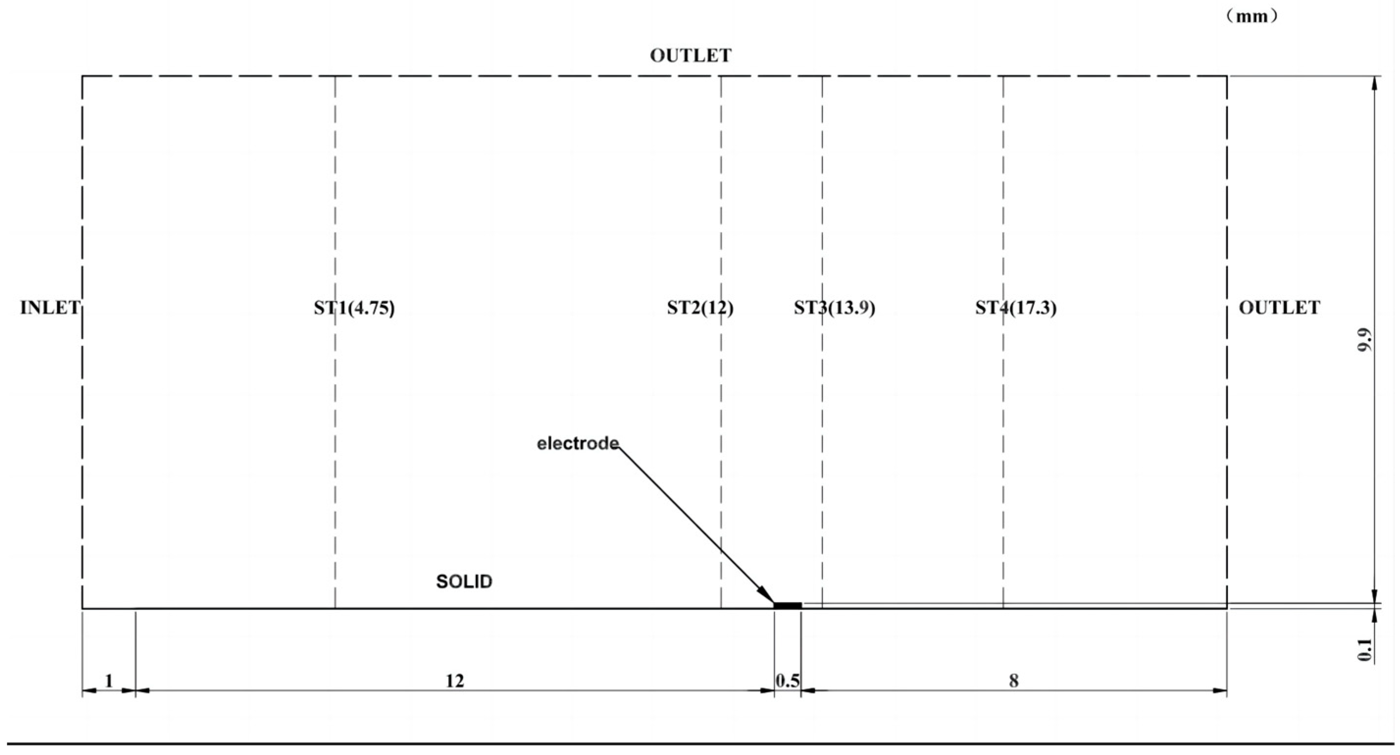
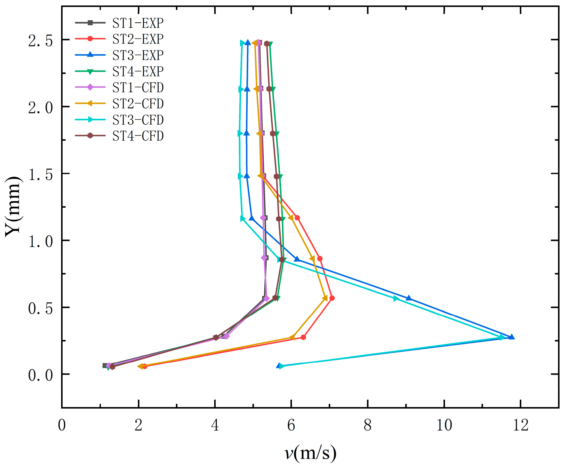
3.2. Validation of the Plasma Actuator Model
4. The High-Speed Cavity Model and Independence Analysis
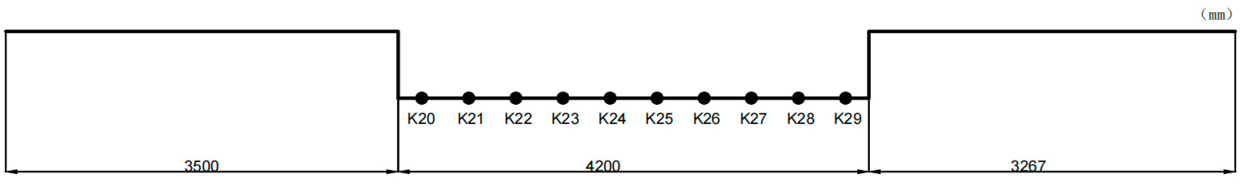
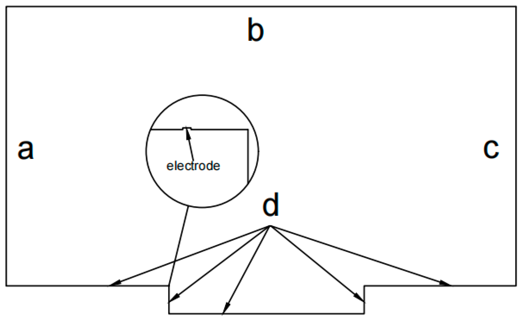
4.1. The Studied High-Speed Cavity Model
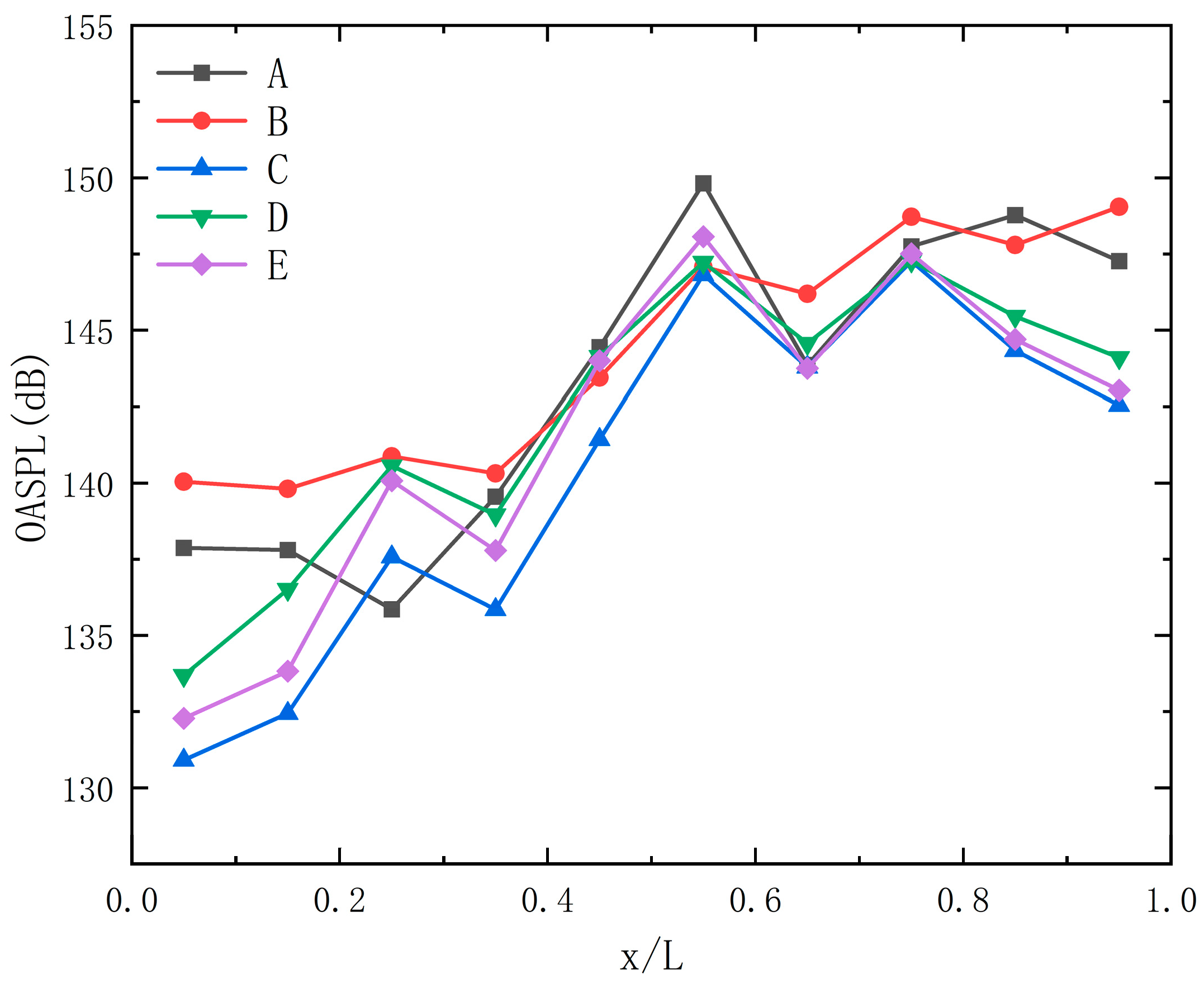
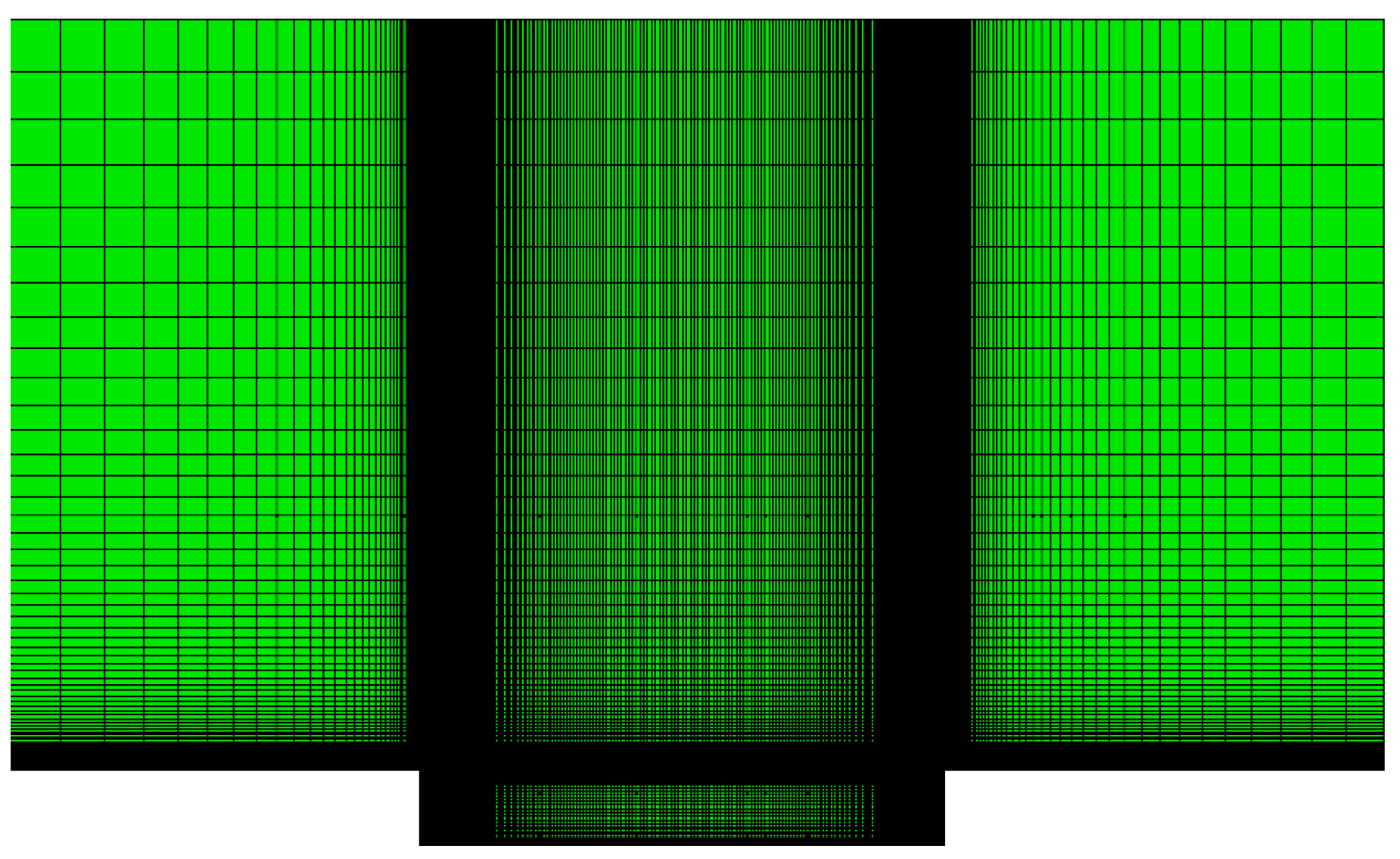
4.2. Grid Independence Analysis
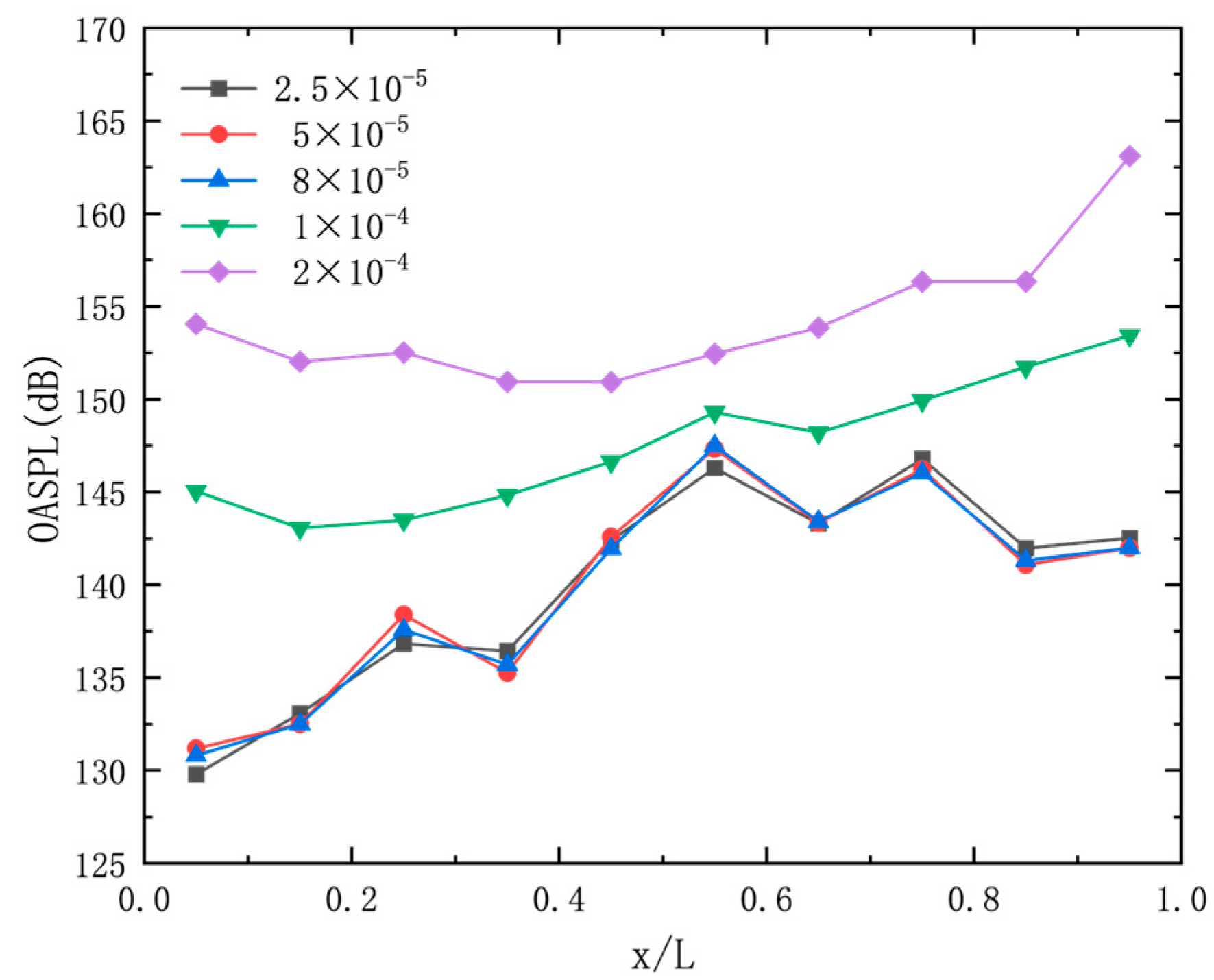
4.3. Time Step Independence Analysis
5. Noise Prediction and Plasma-Based Control of Cavity Flows
5.1. Calculation Setups
5.2. Aerodynamic and Acoustic Characteristics of the Uncontrolled Cavity
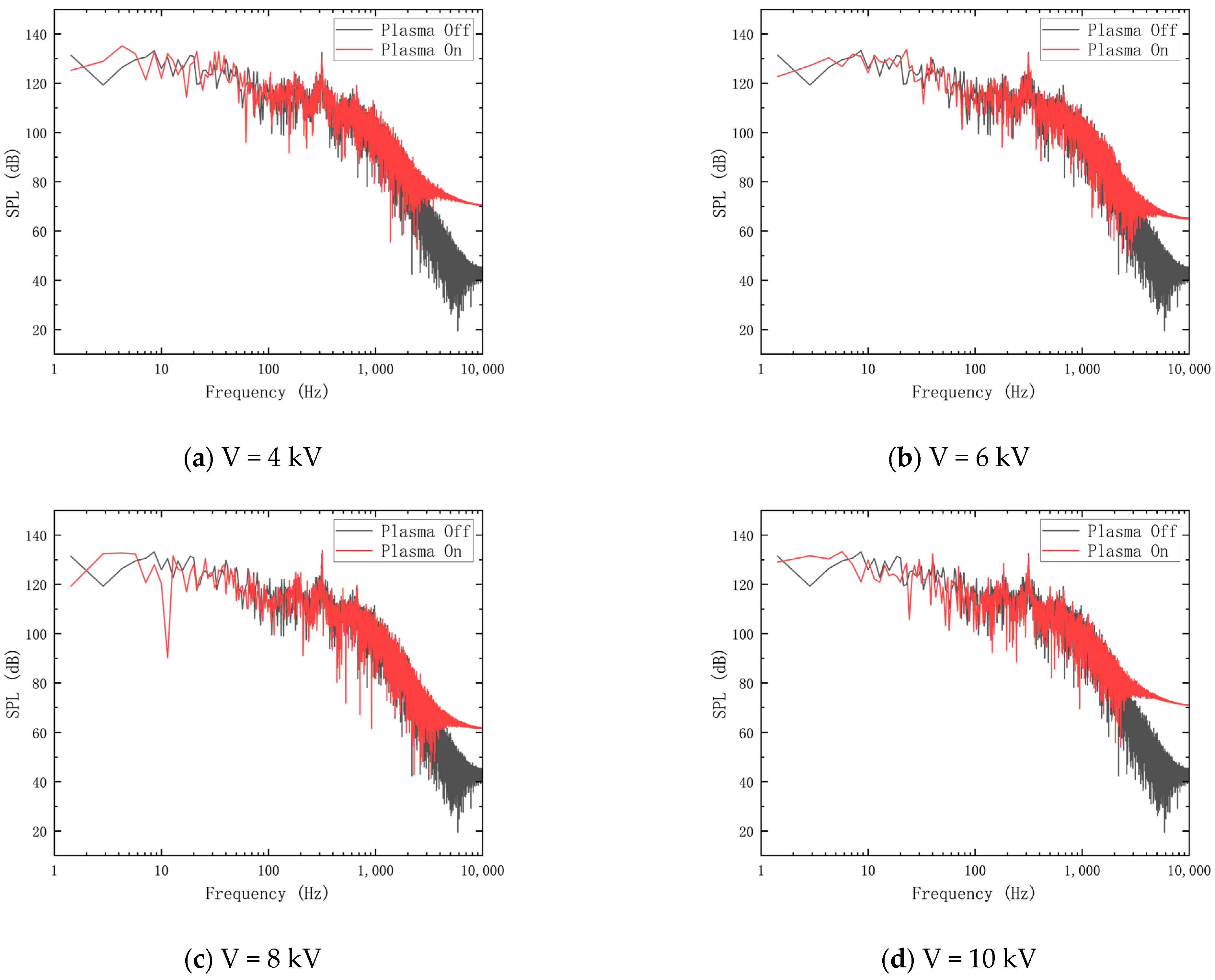
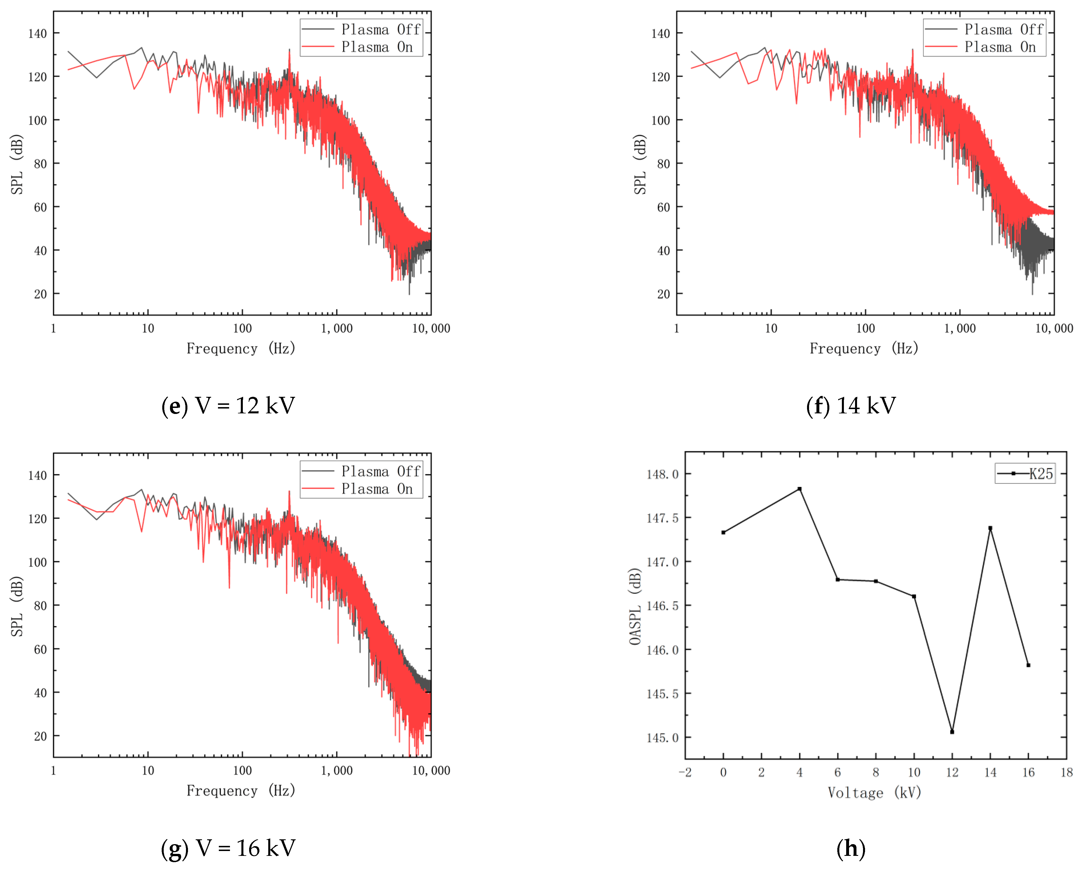
5.3. Influence of Excitation Voltage
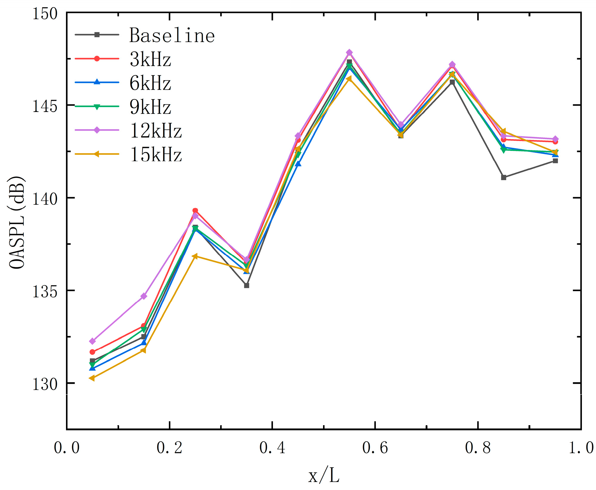
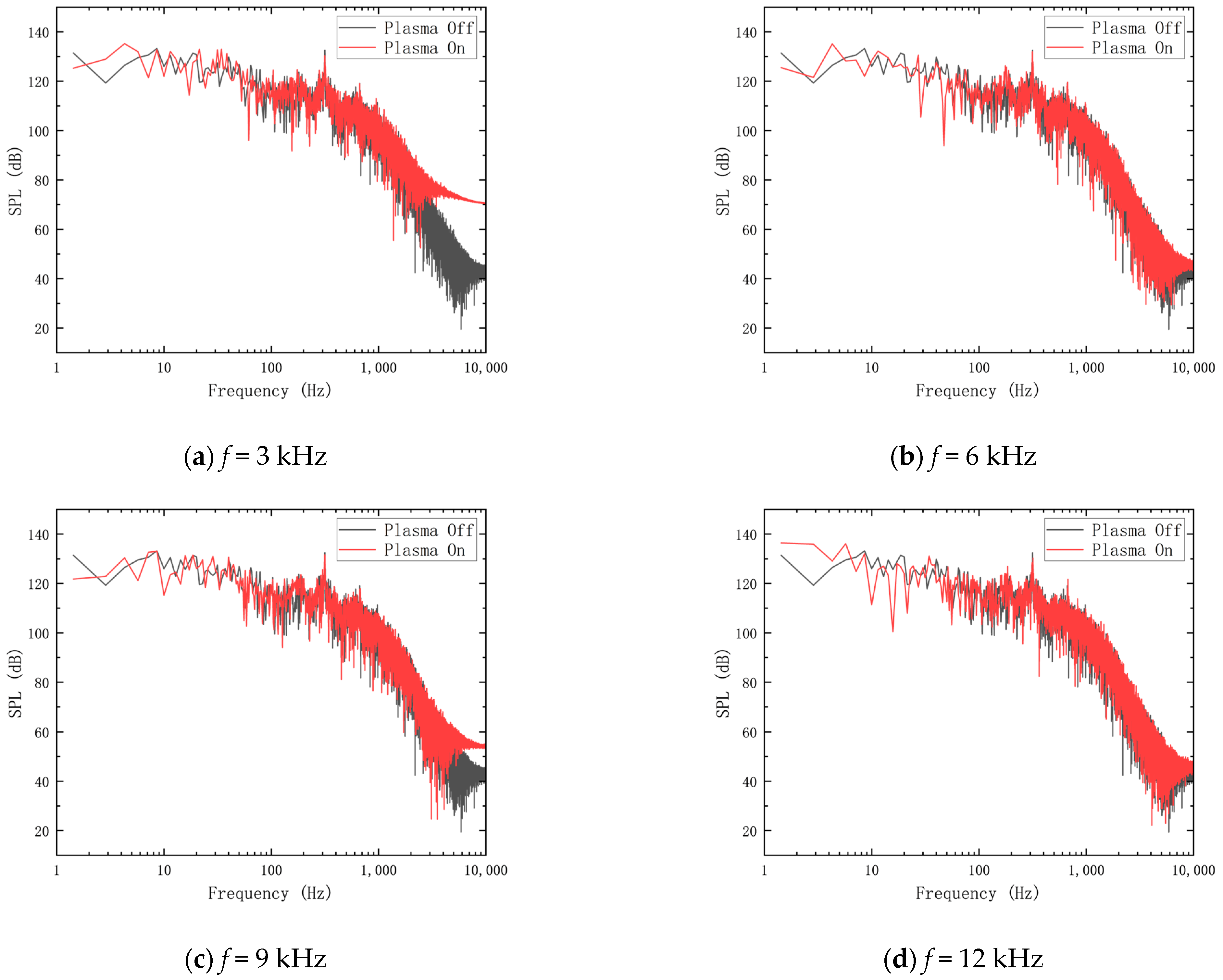
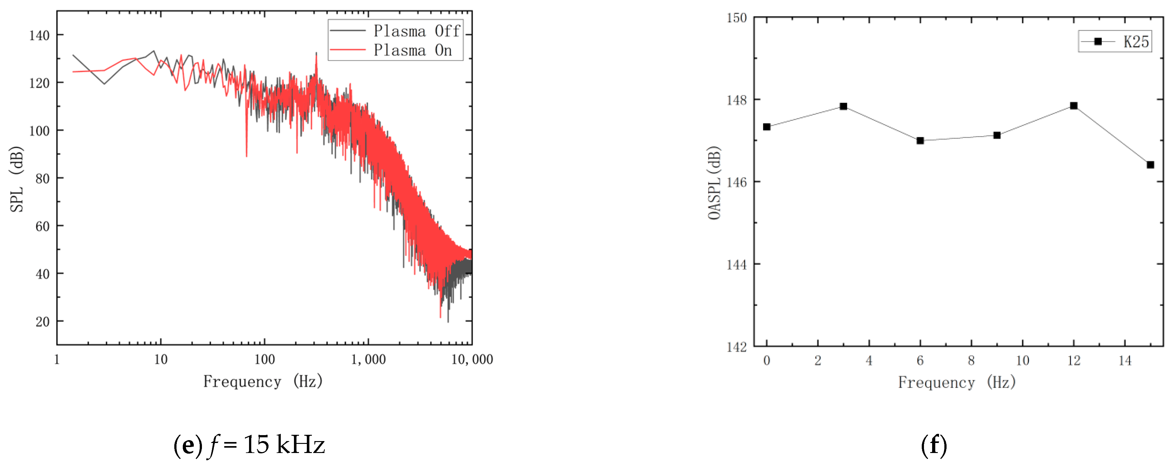
5.4. Effect of Excitation Frequency
6. Conclusions
- This paper studies the suppression of aerodynamic noise in high-speed cavities using a combined DDES and DBD method for the first time. Comparing with experimental data, the calculation error of the OASPL in high-speed cavities is within 2%, and the calculation error of the X-direction velocity of the plasma actuator model is within 9%.
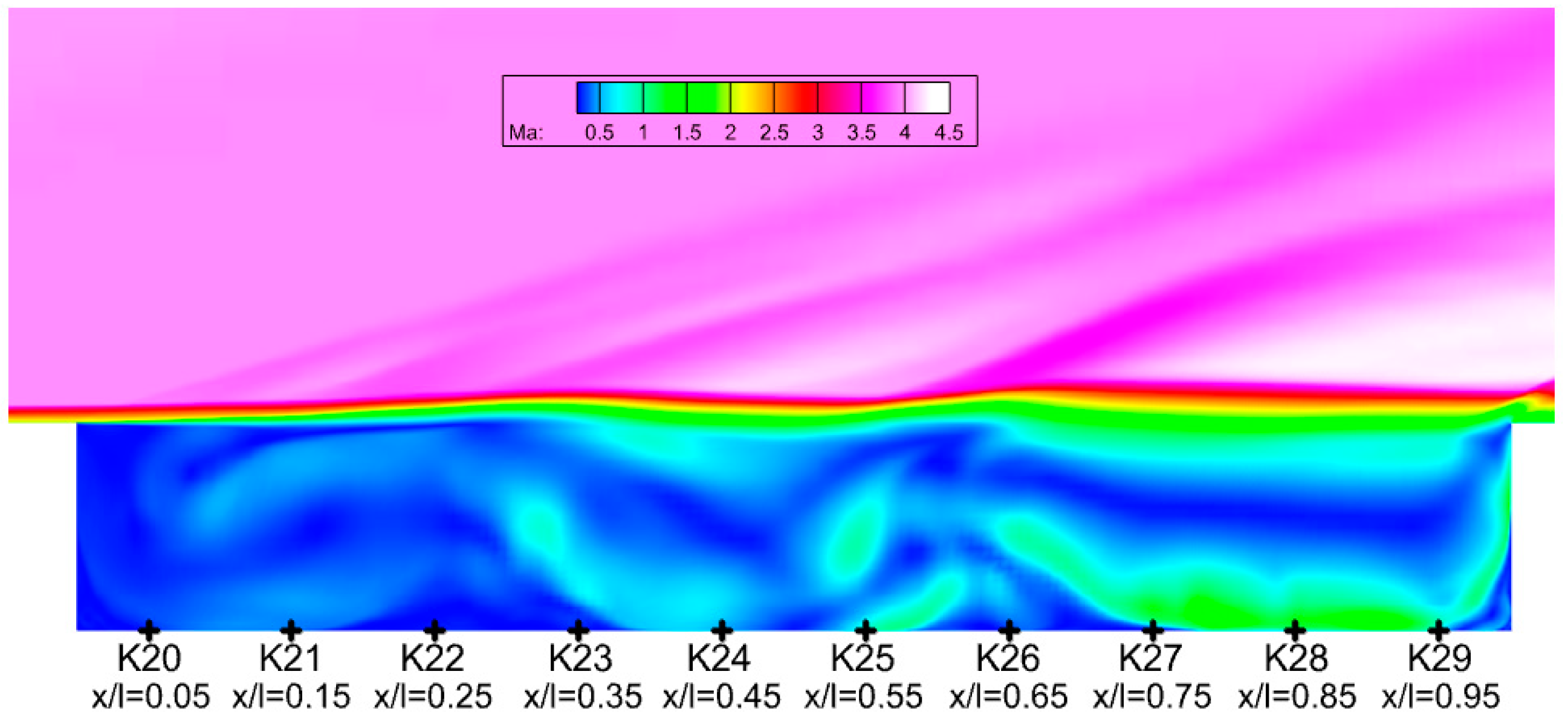
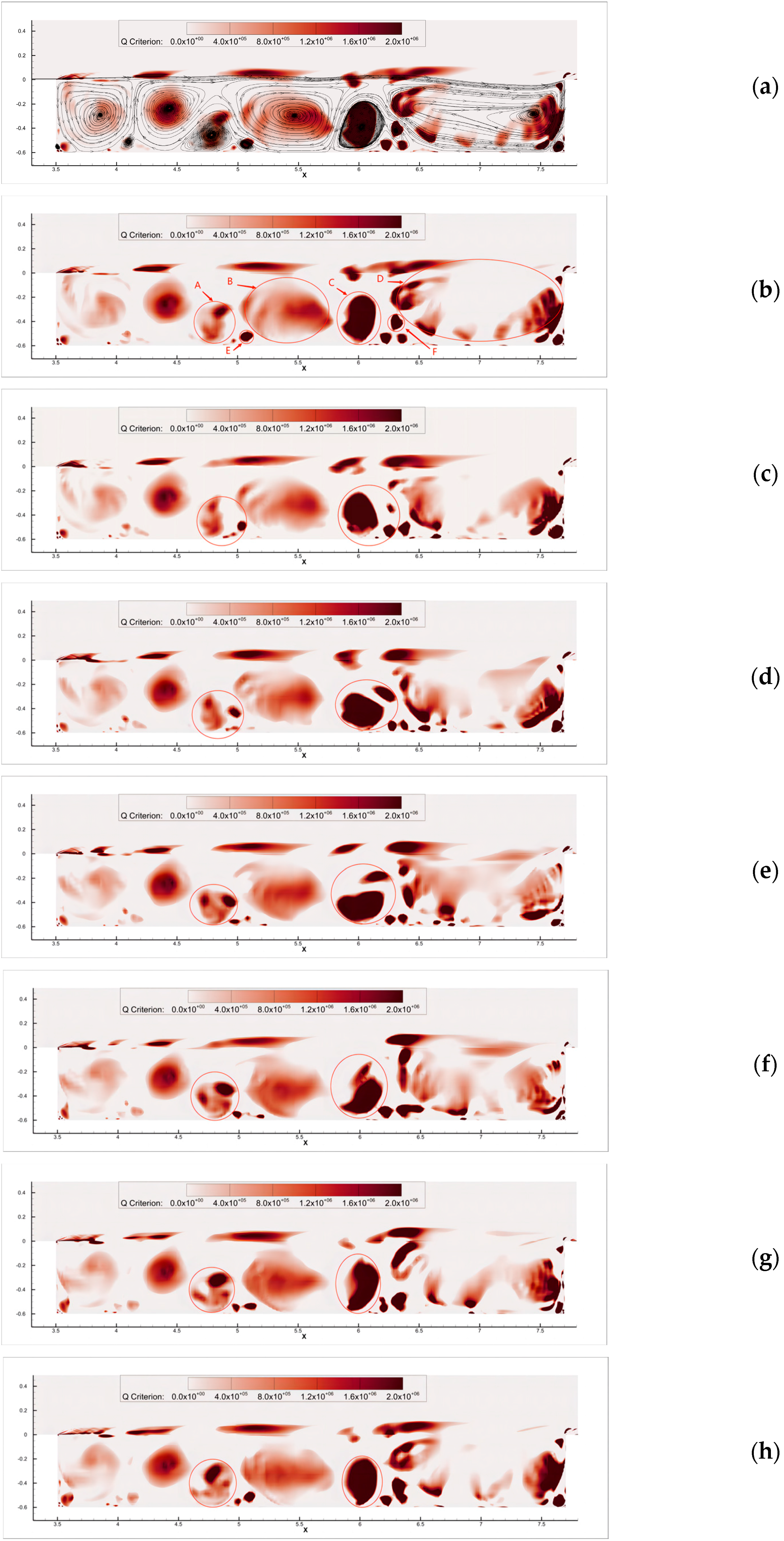
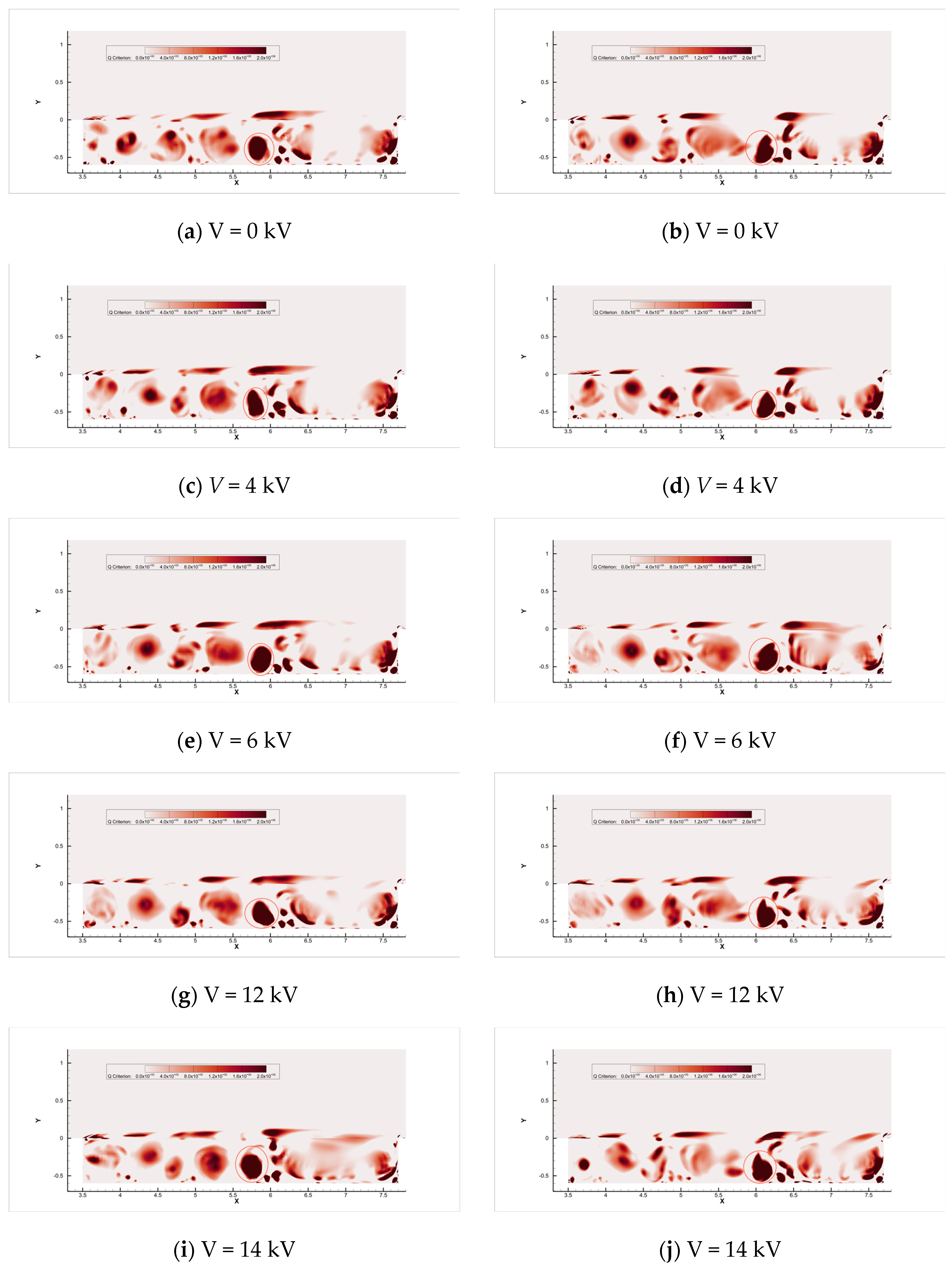
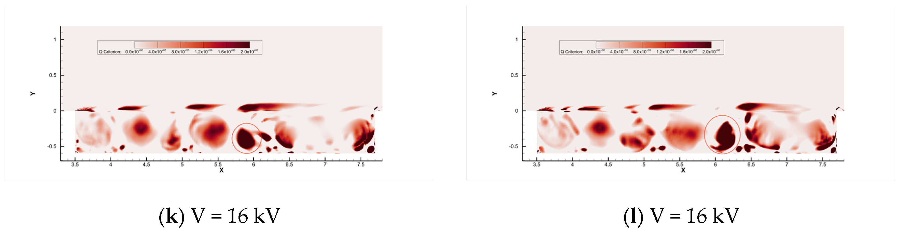
- The cavity with L/D = 7 exhibits distinct open flow characteristics at Ma=4 and an altitude of 25 km. Multiple OASPL peaks are observed in the front, middle, and rear regions of the cavity. The maximum OASPL reaches 147.329 dB, occurring at x/L = 0.55. The locations of vortex breakdown and fusion correspond to the regions and roughly align with regions where extreme values of cavity noise occur.
- Relative to the excitation frequency, the excitation voltage of the plasma actuator has a more pronounced effect on noise suppression. Appropriate excitation voltage can reduce the OASPL by up to 2.27 dB by suppressing low-frequency noise. The excitation voltage can reduce the sound pressure level amplitude of the dominant mode, thereby decreasing the OASPL of the high-speed cavity.
- The effect of the excitation frequency of the plasma actuator on noise suppression is weaker, yet an optimal frequency exists. Variations in the excitation frequency have a less noticeable impact on the frequency and sound pressure level amplitude of the dominant mode, primarily affecting high-frequency sound pressure levels, with a maximum reduction of 0.336 dB in the OASPL.
- Plasma actuators can alter the lateral movement range of the dominant vortex within the high-speed cavity. As the lateral displacement of the dominant vortex decreases, the OASPL of the cavity also decreases.
Author Contributions
Funding
Data Availability Statement
Conflicts of Interest
References
- Rowley, C.W.; Williams, D.R. Dynamics and Control of High-Reynolds-Number Flow over Open Cavities. Annu. Rev. Fluid Mech. 2006, 38, 251–276. [Google Scholar] [CrossRef]
- Heller, H.; Delfs, J. Cavity Pressure Oscillations: Cavity Pressure Oscillations: The Generating Mechanism Visualized. Lett. Ed. J. Sound Vib. 1996, 196, 248–252. [Google Scholar] [CrossRef]
- Lee, B.H.K. Effect of Captive Stores on Internal Weapons Bay Floor Pressure Distributions. J. Aircr. 2010, 47, 732–736. [Google Scholar] [CrossRef]
- Lawson, S.J.; Barakos, G.N. Review of Numerical Simulations for High-Speed, Turbulent Cavity Flows. Prog. Aerosp. Sci. 2011, 47, 186–216. [Google Scholar] [CrossRef]
- Knotts, B.D.; Selamet, A. Suppression of Flow–Acoustic Coupling in Sidebranch Ducts by Interface Modification. J. Sound Vib. 2003, 265, 1025–1045. [Google Scholar] [CrossRef]
- Zhuang, N. Experimental Investigation of Supersonic Cavity Flows and their Control. Ph.D. Thesis, The Florida State University, Tallahassee, FL, USA, 2007. Available online: https://www.proquest.com/dissertations-theses/experimental-investigation-supersonic-cavity/docview/304872228/se-2 (accessed on 24 October 2023).
- Heller, H.; Bliss, D.B. Aerodynamically Induced Pressure Oscillations in Cavities: Physical Mechanisms and Suppression Concepts; Wright-Patterson Air Force Base: Dayton, OH, USA, 1975. [Google Scholar]
- Schmit, R.; Semmelmayer, F.; Grove, J.; Haverkamp, M. Fourier Analysis of High Speed Shadowgraph Images Around a Mach 1.5 Cavity Flow Field. In Proceedings of the 29th AIAA Applied Aerodynamics Conference, Honolulu, HI, USA, 27–30 June 2011; American Institute of Aeronautics and Astronautics: Washington, DC, USA, 1996. [Google Scholar] [CrossRef]
- Handa, T.; Miyachi, H.; Kakuno, H.; Ozaki, T. Generation and Propagation of Pressure Waves in Supersonic Deep-Cavity Flows. Exp. Fluids 2012, 53, 1855–1866. [Google Scholar] [CrossRef]
- Unalmis, O.H.; Clemens, N.T.; Dolling, D.S. Cavity Oscillation Mechanisms in High-Speed Flows. AIAA J. 2004, 42, 2035–2041. [Google Scholar] [CrossRef]
- Rizzetta, D.P. Numerical simulation of supersonic flow over a three-dimensional cavity. AIAA J. 1988, 26, 799–807. [Google Scholar] [CrossRef]
- Chang, K.-S.; Park, S.O. Hybrid RANS/LES Simulation of Deep Cavity Flow. In Proceedings of the 42nd AIAA Aerospace Sciences Meeting and Exhibit, Reno, NV, USA, 5–8 January 2004; American Institute of Aeronautics and Astronautics: Washington, DC, USA, 1996. [Google Scholar] [CrossRef]
- Davidson, L.; Peng, S.H. Hybrid LES–RANS Modelling: A One–equation SGS Model Combined with a k – ω Model for Predicting Recirculating Flows. Int. J. Numer. Methods Fluids 2003, 43, 1003–1018. [Google Scholar] [CrossRef]
- Hamed, A.; Basu, D.; Das, K. Detached Eddy Simulations of Supersonic Flow over Cavity. In Proceedings of the 41st Aerospace Sciences Meeting and Exhibit, Reno, NV, USA, 6–9 January 2003; American Institute of Aeronautics and Astronautics: Washington, DC, USA, 1996. [Google Scholar] [CrossRef]
- Tang, Y.; Luo, L.; Zhang, P.; Ma, M. Effect of Rear Wall Inclination on Cavity Acoustic Characteristics at High Mach Numbers. J. Phys. Conf. Ser. 2022, 2252, 012007. [Google Scholar] [CrossRef]
- Jin, X.; Huang, F.; Miao, W.; Cheng, X.; Wang, B. Effects of the boundary-layer thickness at the cavity entrance on rarefied hypersonic flows over a rectangular cavity. Phys. Fluids 2021, 33, 036116. [Google Scholar] [CrossRef]
- Larsson, J.; Davidson, L.; Olsson, M.; Eriksson, L.-E. Aeroacoustic Investigation of an Open Cavity at Low Mach Number. AIAA J. 2004, 42, 2462–2473. [Google Scholar] [CrossRef]
- Lawson, S.J.; Barakos, G.N. Computational Fluid Dynamics Analyses of Flow over Weapons-Bay Geometries. J. Aircr. 2010, 47, 1605–1623. [Google Scholar] [CrossRef]
- Zhang, X.; Chen, X.; Rona, A.; Edwards, J. Attenuation of cavity flow oscillation through leading edge flow control. J. Sound Vib. 1999, 221, 23–47. [Google Scholar] [CrossRef]
- Zhuang, N.; Alvi, F.S.; Alkislar, M.B.; Shih, C. Supersonic Cavity Flows and Their Control. AIAA J. 2006, 44, 2118–2128. [Google Scholar] [CrossRef]
- Vakili, A.D.; Gauthier, C. Control of cavity flow by upstream mass-injection. J. Aircr. 1994, 31, 169–174. [Google Scholar] [CrossRef]
- Luo, K.; Zhe, W.; Xiao, Z.; Fu, S. Improved delayed detached-eddy simulations of sawtooth spoiler control before supersonic cavity. Int. J. Heat Fluid Flow 2017, 63, 172–189. [Google Scholar] [CrossRef]
- Alam, M.; Matsuob, S.; Teramotob, K.; Setoguchib, T.; Kim, H.-D. A new method of controlling cavity-induced pressure oscillations using sub-cavity. J. Mech. Sci. Technol. 2007, 21, 1398–1407. [Google Scholar] [CrossRef]
- Schmit, R.; Semmelmayer, F.; Haverkamp, M.; Grove, J.; Ahmed, A. Examining Passive Flow Control Devices with High Speed Shadowgraph Images around a Mach1.5 Cavity Flow Field. In Proceedings of the 6th AIAA Flow Control Conference, New Orleans, LA, USA, 25–28 June 2012; American Institute of Aeronautics and Astronautics: Washington, DC, USA, 1996. [Google Scholar] [CrossRef]
- Danilov, P.; Quackenbush, T. Flow Driven Oscillating Vortex Generators for Control of Cavity Resonance. In Proceedings of the 49th AIAA Aerospace Sciences Meeting Including the New Horizons Forum and Aerospace Exposition, Orlando, FL, USA, 4–7 January 2011; American Institute of Aeronautics and Astronautics: Washington, DC, USA, 1996. [Google Scholar] [CrossRef]
- Thangamani, V.; Saddington, A.; Knowles, K. An Investigation of Passive Control Methods for a Large Scale Cavity Model in High Subsonic Flow. In Proceedings of the 19th AIAA/CEAS Aeroacoustics Conference, Berlin, Germany, 24 May 2013; American Institute of Aeronautics and Astronautics: Washington, DC, USA, 1996. [Google Scholar] [CrossRef]
- Vikramaditya, N.S.; Kurian, J. Pressure Oscillations from Cavities with Ramp. AIAA J. 2009, 47, 2974–2984. [Google Scholar] [CrossRef]
- Spalart, P.R. Comments on the Feasibility of LES for Wings, and on a Hybrid RANS/LES Approach. In Proceedings of the First AFOSR International Conference on DNS/LES, Ruston, Louisiana, LA, USA, 4–8 August 1997. [Google Scholar]
- Baldwin, B.; Lomax, H.T.-l. Approximation and Algebraic Model for Separated Turbulentflows. In Proceedings of the 16th Aerospace Sciences Meeting, Huntsville, AL, USA, 16–18 January 1978; American Institute of Aeronautics and Astronautics: Washington, DC, USA, 1996. [Google Scholar] [CrossRef]
- Larcheveque, L.; Sagaut, P.; Lê, T.-H. Large-Eddy Simulations of Flows in Weapon Bays. In Proceedings of the 41st Aerospace Sciences Meeting and Exhibit, Reno, NV, USA, 6–9 January 2003; American Institute of Aeronautics and Astronautics: Washington, DC, USA, 1996. [Google Scholar] [CrossRef]
- Rodriquez, G.; Carlos, V.; Marcel, I. Numerical Studies of High-Speed Cavity Flows Using LES, DDES and IDDES. In Proceedings of the 51st AIAA Aerospace Sciences Meeting Including the New Horizons Forum and Aerospace Exposition, Orlando, LA, USA, 1 January 2013. [Google Scholar]
- Shyy, W.; Jayaraman, B.; Andersson, A. Modeling of glow discharge-induced fluid dynamics. J. Appl. Phys. 2002, 92, 6434–6443. [Google Scholar] [CrossRef]
- Sinha, N.; Dash, S.; Chidambaram, N.; Findlay, D. A Perspective on the Simulation of Cavity Aeroacoustics. In Proceedings of the 36th AIAA Aerospace Sciences Meeting and Exhibit, Reno, NV, USA, 12–15 January 1998; American Institute of Aeronautics and Astronautics: Reno, NV, USA, 2012. [Google Scholar] [CrossRef]
- Bauer, R.C.; Dix, R.E. Engineering Model of Unsteady Flow in a Cavity; Arnold Engineering Development Center, US Air Force: Arnold AFB, TN, USA, 1991. [Google Scholar]


| Modal | |||||
|---|---|---|---|---|---|
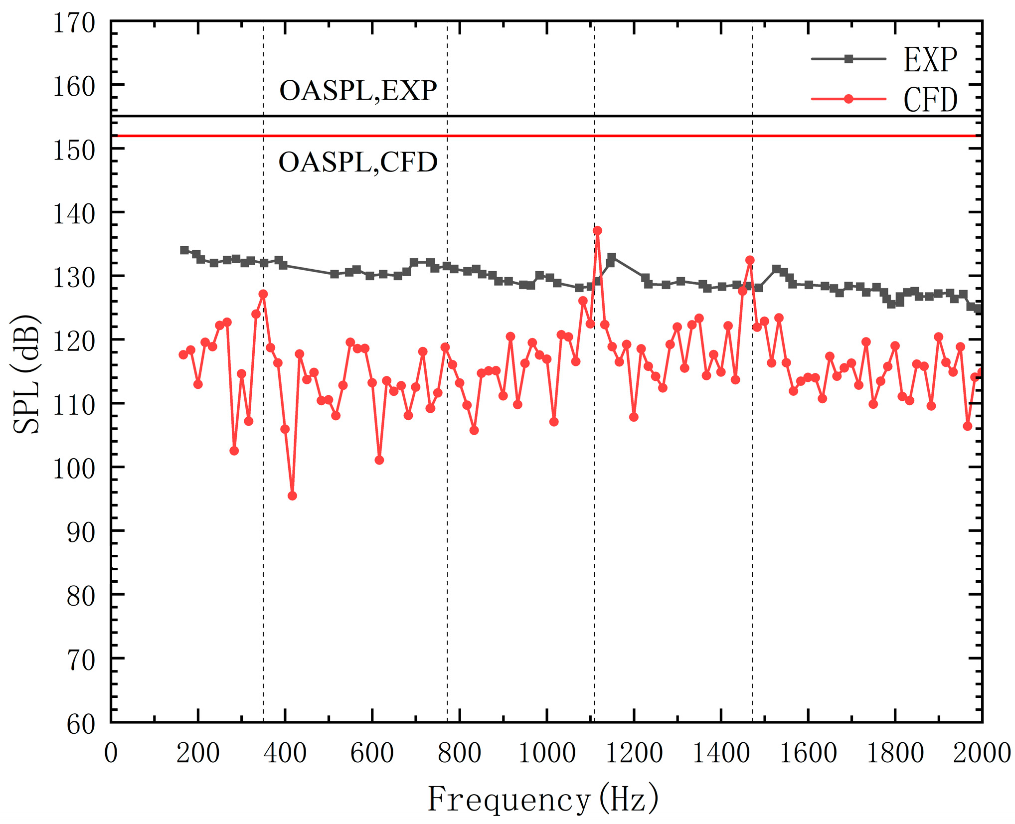
| Experiment | Frequency (Hz) | 287 | 695 | 1152 | 1527 |
| Sound Pressure Level (dB) | 132.5 | 132.1 | 132.8 | 131 | |
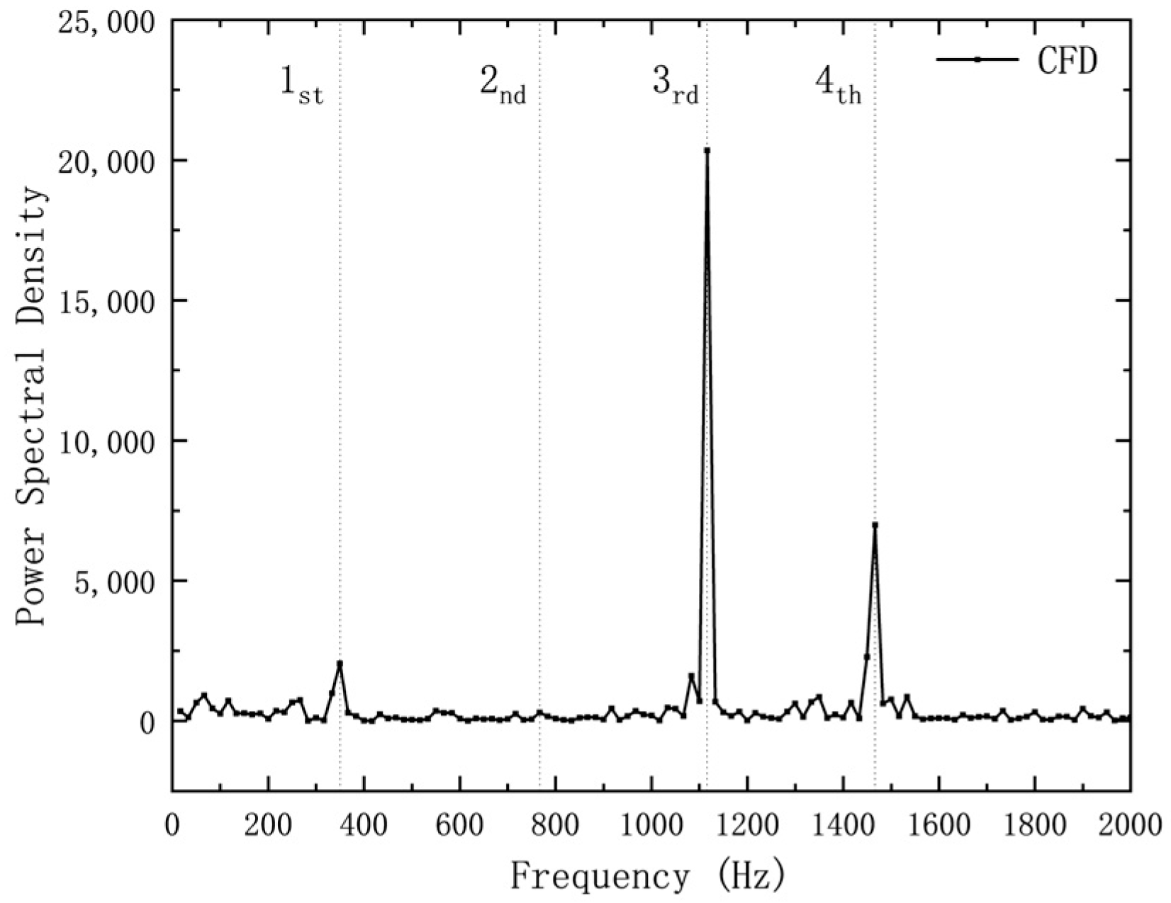
| CFD | Frequency (Hz) | 349.9 | 766.5 | 1116 | 1466.4 |
| Sound Pressure Level (dB) | 127.1 | 118.8 | 137.1 | 132.4 | |
| Case | 1 | 2 | 3 | 4 | 5 | 6 | 7 |
|---|---|---|---|---|---|---|---|
| Excitation Frequency (kHz) | 3 | ||||||
| Excitation Voltage (kV) | 4 | 6 | 8 | 10 | 12 | 14 | 16 |
| Excitation Voltage (kV) | 0 | 4 | 6 | 12 | 14 | 16 |
|---|---|---|---|---|---|---|
| OASPL (dB) | 147.329 | 147.827 | 146.791 | 145.057 | 147.38 | 145.819 |
| X-direction Displacement Range (mm) | 304.8 | 347.6 | 276.5 | 239.6 | 338.2 | 267.8 |
| Case | 8 | 9 | 10 | 11 | 12 |
|---|---|---|---|---|---|
| Excitation Voltage (kV) | 4 | ||||
| Excitation Frequency(kHz) | 3 | 6 | 9 | 12 | 15 |
| Excitation Frequency (kHz) | 0 | 3 | 12 | 15 |
|---|---|---|---|---|
| OASPL (dB) | 147.329 | 147.827 | 147.843 | 146.407 |
| X-direction Displacement Range (mm) | 304.8 | 347.6 | 374.9 | 262.5 |
Disclaimer/Publisher’s Note: The statements, opinions and data contained in all publications are solely those of the individual author(s) and contributor(s) and not of MDPI and/or the editor(s). MDPI and/or the editor(s) disclaim responsibility for any injury to people or property resulting from any ideas, methods, instructions or products referred to in the content. |
© 2023 by the authors. Licensee MDPI, Basel, Switzerland. This article is an open access article distributed under the terms and conditions of the Creative Commons Attribution (CC BY) license (https://creativecommons.org/licenses/by/4.0/).
Share and Cite
Cai, H.; Zhang, Z.; Li, Z.; Li, H. Noise Prediction and Plasma-Based Control of Cavity Flows at a High Mach Number. Aerospace 2023, 10, 922. https://doi.org/10.3390/aerospace10110922
Cai H, Zhang Z, Li Z, Li H. Noise Prediction and Plasma-Based Control of Cavity Flows at a High Mach Number. Aerospace. 2023; 10(11):922. https://doi.org/10.3390/aerospace10110922
Chicago/Turabian StyleCai, Hongming, Zhuoran Zhang, Ziqi Li, and Hongda Li. 2023. "Noise Prediction and Plasma-Based Control of Cavity Flows at a High Mach Number" Aerospace 10, no. 11: 922. https://doi.org/10.3390/aerospace10110922
APA StyleCai, H., Zhang, Z., Li, Z., & Li, H. (2023). Noise Prediction and Plasma-Based Control of Cavity Flows at a High Mach Number. Aerospace, 10(11), 922. https://doi.org/10.3390/aerospace10110922