Integrating GRU with a Kalman Filter to Enhance Visual Inertial Odometry Performance in Complex Environments

Abstract

To enhance system reliability and mitigate the vulnerabilities of the Global Navigation Satellite Systems (GNSS), it is common to fuse the Inertial Measurement Unit (IMU) and visual sensors with the GNSS receiver in the navigation system design, effectively enabling compensations with absolute positions and reducing data gaps. To address the shortcomings of a traditional Kalman Filter (KF), such as sensor errors, an imperfect non-linear system model, and KF estimation errors, a GRU-aided ESKF architecture is proposed to enhance the positioning performance. This study conducts Failure Mode and Effect Analysis (FMEA) to prioritize and identify the potential faults in the urban environment, facilitating the design of improved fault-tolerant system architecture. The identified primary fault events are data association errors and navigation environment errors during fault conditions of feature mismatch, especially in the presence of multiple failure modes. A hybrid federated navigation system architecture is employed using a Gated Recurrent Unit (GRU) to predict state increments for updating the state vector in the Error Estate Kalman Filter (ESKF) measurement step. The proposed algorithm’s performance is evaluated in a simulation environment in MATLAB under multiple visually degraded conditions. Comparative results provide evidence that the GRU-aided ESKF outperforms standard ESKF and state-of-the-art solutions like VINS-Mono, End-to-End VIO, and Self-Supervised VIO, exhibiting accuracy improvement in complex environments in terms of root mean square errors (RMSEs) and maximum errors.

1. Introduction

In recent years, unmanned aerial vehicles (UAVs) have gained attraction with the evolution of technologies such as artificial intelligence and computer vision, which have effectively broadened pathways for diverse applications and services. UAVs have been utilized in many civil applications, such as aerial surveillance, package delivery, precision agriculture, search and rescue operations, traffic monitoring, remote sensing, and post-disaster operations [1]. The increasing demand for commercial UAVs for such applications has highlighted the need for robust, secure, and accurate navigation solutions. However, achieving accurate and reliable UAV positioning in complex environments, including overpasses, urban canyons, illumination variability, etc., has become more challenging.

Although Global Navigation Satellite Systems (GNSS) have become one of the most popular navigation systems in recent decades, the utilization of GNSS remains suspicious due to its vulnerability to satellite visibility, interference of jamming and spoofing, as well as environmental effects such as multipath, building mask, ionospheric and tropospheric delays. Furthermore, the effects will lead to sharp deteriorations in the positioning precision and GNSS availability [2]. The inertial navigation system (INS) facilitates the provision of high-frequency and continuous position, velocity, and attitude information, which makes the integration of INS with GNSS prevalent in most navigation architecture designs. However, the drift error generated from INS accumulates over time, which will result in divergent positioning output. The impact of INS drifting on GNSS/INS fusion performance in the case of long-term GNSS outages has been explored widely [3,4,5]. Nevertheless, more sensor types are still in demand to provide more resilient and accurate positioning resolutions under complex operation scenarios.

The vision-based navigation system is a promising alternative for providing reliable positioning information without radio frequency interference effects during GNSS outages. Visual odometry (VO) is frequently employed as a critical component in the vision-based navigation system due to its efficient deployment with low computational complexity in contrast to Visual Simultaneous Localization and Mapping (VSLAM). The Visual Inertial Navigation Systems (VINS) have been fully explored by researchers, encompassing notable examples like VINS-Mono [6], MSCKF [7], ORB-SLAM3 [8], and open-VINS [9]. As a common solution for improving navigation performance in terms of accuracy, integrity, update rate, and robustness through adding sensor types with GNSS, the VINS navigation system with multiple integrated sensors presents a higher possibility of existing multiple faults, noise, and sensor failures within the system. It was discovered that purely VO-enabled navigation presents performance degradation caused by factors such as illumination, motion blur, field of view, moving objects, and texture environment [10]. As a result, there is a need to explore fault-tolerant designs in the VINS navigation systems to mitigate the fault impact on the visual systems.

For achieving the fault tolerance capability in integrated multi-sensor systems, the decentralized filtering design, especially using federated architecture, has become popular in recent years. Dan et al. [11] proposed an adaptive positioning algorithm based on a federated Kalman filter combined with a robust Error Estate Kalman Filter (ESKF) with adaptive filtering for the UAV-based GNSS/IMU/VO navigation system to eliminate issues of GNSS signal interruption and lack of sufficient feature points while navigating in indoor and outdoor environments. However, most papers using ESKF only measure VO faults by adding position errors, whilst faults coming from visual cues like scarcity of features caused by environment complexity and motion dynamics or high non-linearity characteristics have not been fully taken into account. Therefore, there is a gap in detecting and identifying faults and threats with consideration of visual cues in the GNSS/IMU/VO navigation system.

Current state-of-the-art fault-tolerant GNSS/IMU/VO navigation systems encounter more difficulties when operating in complex scenarios due to the challenges of identifying visual failure modes and correcting VO errors. As a structured and systematic fault identification method, Failure Mode and Effect Analysis (FMEA) is capable of identifying various fault types, defects, and sensor failures based on predicted and measured values as they occur instantly or shortly after they occur. FMEA is commonly used to assess risks to improve the reliability of complex systems by identifying and evaluating potential failures with the provision of occurrence likelihood, severity of impact, and detectability, as well as prioritizing high-risk failure modes. However, researchers working on VIO discussed several faults caused by navigation environment or sensor error individually [10,12,13], but identifying failure modes is a gap. Moreover, despite their extracted failure modes, systematic faults have not been discovered with only the consideration of single or specific combined faults like motion blur, rapid motion, and illumination variation.

To resolve the inherent non-linearity in the visual navigation system, AI has been employed with a Kalman filter to enhance the ability to model temporal changes in sensor data. Nevertheless, AI has the disadvantages of training time and predicted value inevitability containing errors that can be partially resolved by simplifying the neural network, for example, with a Gradient Recurrent Unit (GRU) suppressed with ESKF fusion, thus enabling ESKF to better handle scenarios with verifying level of uncertainty and dynamic sensor conditions.

To implement a fault tolerance navigation system against the visually degraded environment, this paper proposes a GRU-aided ESKF VIO algorithm that conducts FMEA on the VINS system to identify failure modes and then assists the architecture of fault-tolerant multi-sensor system where the AI-aided ESKF VIO integration is used as one of the sub-filters to correct identified visual failure modes. The major contributions of this paper are highlighted as follows:

• The proposition of an FMEA-supported fault-tolerant federated GNSS/IMU/VO integrated navigation system. The FMEA execution on an integrated VINS system contributes to enhancing the system’s design, with a focus on accurate navigation during GNSS outages.
• The proposition of a GRU-based enhancement of ESKF for predicting increments of positions to update measurements of ESKF, aiming to correct visual positioning errors, leading to more accurate and robust navigation in challenging conditions.
• Performance evaluation of GRU-aided ESKF-based VIO within the fault-tolerant GNSS/IMU/VO multi-sensor navigation system. Training datasets for the GRU model are selected to replicate the failure modes extracted with fault conditions from FMEA. The verification is simulated and benchmarked on the Unreal engine, where the environment includes complex scenes of sunlight, shadow, motion blur, lens blur, no-texture, light variation, and motion variation. The validation dataset is grouped into multiple zone categories in accordance with single or multiple fault types due to environmental sensitivity and dynamic motion transitions.
• The performance of the proposed algorithm is compared with the state-of-the-art End-to-End VIO and Self-supervised VIO by testing similar datasets on the proposed algorithm.

The remaining part of the paper is organized as follows. Section 2 discusses the existing systems designed based on a hybrid approach; Section 3 introduces the proposed GRU-aided KF-based federated GNSS/INS/VO navigation System; Section 4 discusses the experimental setup; Section 5 discusses the roast test, and result analysis comparison with state-of-the-art systems, and the conclusion is presented in Section 6.

2. Related Works

2.1. Kalman Filter for VIO

A Kalman Filter (KF), along with its variations, is a traditional method that can efficiently fuse VO and IMU information. Despite its effectiveness, the KF faces certain challenges that can impact its performance. One of the main challenges in navigation applications arising from VO vulnerability is the interruption in updating KF observation, leading to a gradual decline in system performance over time. Moreover, if the error characteristics are non-Gaussian and cannot be fully described within the model, the KF may struggle to provide an accurate estimation.

Some studies aim to improve the fusion robustness against non-linear natures from high system dynamics and complex environments, variants of Kalman filter such as the Extended Kalman Filter (EKF) [14,15,16,17], Multi-state Constraint Kalman Filter (MSCKF) [18,19,20,21,22], Unscented Kalman Filter (UKF) [23], Cubature Kalman filter (CKF) [24,25], and Particle Kalman Filter (PF) [26], have been proposed and evaluated. One challenge in the EKF-based VIO navigation system is handling significant non-linearity during brightness variations [15,17] and dynamic motion [15], which will cause feature-matching errors and degrade the overall performance. When these feature-matching errors occur, the EKF’s assumption about linear system dynamics and Gaussian noise may no longer hold, leading to suboptimal states and even filter divergences. To improve VIO performance under brightness variation and significant non-linearities, MSCKF was proposed and evaluated in complex environments such as insufficient light [19,20,21,22], texture missing [19,21], and camera jitter [19] specifically characterized by blurry images [22]. However, in the MSCKF algorithm, the visual features are mostly treated as separate states, so the process is delayed until all visual features are obtained. Another approach is proposed to handle additive noise: VIO uses camera observation to update the filter, allowing for avoiding over-parameterization and helping to reduce growth caused by UKF [23]. In most studies like [24,25], researchers have not focused on evaluating their proposed algorithms among complex scenarios such as light variation, rapid motion, motion blur, overexposures, and field of view, which deteriorate the accuracy and robustness of the state estimation.

Nevertheless, in GNSS-denied scenarios, UAV navigation predominantly depends on VIO, so the challenges remain unresolved using KF variations only for VIO applications. Therefore, the use of ESKF-based VIO for performance improvement is highlighted through alleviating challenges by managing parameter constraints, mitigating singularity and gimbal lock concerns, maintaining parameter linearization, and supporting sensor integration in this paper.

2.2. Hybrid Fusion Enhanced by AI

A number of artificial techniques, such as neural networks, including Deep Neural Networks (DNN), Artificial Neural Networks (ANN), and Reinforcement Learning (RL), have been studied for sensor fusion applications to formulate hybrid fusion solutions. Kim et al. [27] conducted a detailed review of KF with AI techniques to enhance the capabilities of the KF and address its specific limitations in various applications. The recent survey [28] summarizes detailed reviews of the GNSS/INS navigation system that utilizes Artificial Neural Networks (ANN) in combination with the Kalman Filter. This survey highlights the advantages of hybrid methods that leverage ANNs to mitigate INS performance degradation during GNSS vulnerability in specific conditions of aerial underwater vehicles [29,30,31] and Doppler underwater navigation [32]. It was found that one advantage of the hybrid fusion scheme is providing the ability to intercorporate a priori knowledge about the level of change in the timer series, enhancing the systems’ adaptability to varying environments and conditions. Additionally, the ANN error predictor proves to be successful in providing extremely precise adjustments to standalone INS when GNSS signals are unavailable, ensuring continuous and accurate navigation. This survey motivates further exploration and development of hybrid fusion-based navigation schemes to maintain robust performance in challenging GNSS-degradation environments.

Figure 1 presents an overview of publications on NN-assisted navigation applications over the 2018–2023 period and categorizes them into KF performance degradation following the category rule defined by Kim et al. [27]. It is concluded that most studies focus on updating the state vector or measurements of KF, ignoring issues arising from imperfect models. Hereby, estimating pseudo-measurements during GNSS outages to update KF measurements using AI is suggested by [27]. In certain scenarios, particularly when dealing with high-non-linear sensors or navigating in complex environments, updating state vectors directly by predicting sensor increments using NN in measurement steps becomes critical regarding the sensor’s complexity and the challenging nature of the environment.

Figure 1. Published articles on hybrid machine learning usage in KF.

To overcome KF drawbacks in navigation, hybrid methods combining AI approaches, especially machine learning (ML) algorithms, become promising by accurate prediction of INS and visual sensor errors from diverse training datasets. As depicted in Figure 1, most publications belong to the category of ‘State Vector or Measurements of KF’, meaning most studies apply ML to predict and compensate for state vector error or measurements in KF. For instance, Zhang et al. [33] used RBFN to predict states in the prediction step. However, studies like [33] predict absolute state vectors instead of vector increments using NN, which increases model complexity and requires a more extensive training process. Studies from [29,32,33,34,35,36,37,38,39,40,41,42,43,44,45] adopted vector increments of the sensor observations and predictions during KF prediction, whilst most of the work only works on GNSS/INS navigation during GNSS outages, aiming for improving INS efficiency INS in urban settings and situations [31,38,39,41,42,46].

Other studies [47,48] corresponding to the error compensation category employ ML to compensate for the navigation performance error with KF, but sensor errors such as the non-linear error model of INS are excluded.

The category called pseudo measurement input applies NN for predicting pseudo-range errors when the occurrence of a shortage of satellite numbers to update measurement steps in CKF [49] and the adaptive EKF [46,50].

The category of parameter tuning of KF aims to enhance the performance using RL by predicting the covariance matrix, such as using AKF in [50]. However, the prediction of the covariance matrix relies on changeable factors like temperature, which is difficult to predict and model. Therefore, using NN for parameter tuning in KF is not considered in this paper.

Regarding the selection of NN types, Radial Basis Factor Neural Networks (RBFNs), Backpropagation Neural Networks (BPNNs), and Extreme Learning Machines (ELMs) are powerful learning algorithms and more suitable for static data or non-sequential problems but neglect the information of historical data. Additionally, navigation applications are inherently time-dependent and dynamic, making them challenging to model using these learning algorithms. Other studies [30,38] have proved RBFN has less complexity than BPNN and multi-layer backpropagation networks, yet haven’t considered any dynamics change over time. Other studies were presented using simple neural networks on SLAM applications by predicting state increments in diverse scenarios.

The authors in [35,36] did not account for the temporal variations in features that can significantly impact the performance, given that basic neural networks are sensitive to such changes. Kotov et al. [37] compared NNEKF-MPL and NNEKF-ELM, demonstrating that NNEKF-MPL performs better when the vehicle exhibits a non-constant systematic error. However, the aforementioned NN methods do not take temporal information contained within historical data into training, making those methods insufficient for addressing navigation applications’ dynamic and time-dependent characteristics.

Some studies have proved the advantages of using time-dependent recurrent NN architectures like Long Short-Term Memory (LSTM) in VIO. VIIONET [51] used LTSM to process high-rate IMU data that concentrated with feature vectors from images processed through CNN. Although adopting IMUs can facilitate the mitigation of IMU dynamic errors, the compensation of visual cues in VIO affected by complex environmental conditions is more critical. DynaNet [52] was the first to apply LSTM-aided EKF to show hybrid mechanism benefits in improving motion prediction performance on VO and VIO without sufficient visual features. Furthermore, this study suggested unresolved challenges of motion estimation tasks, multi-sensor fusion under data absence, and data prediction in visual degradation scenarios. Subsequently, researchers aim to learn VO positions from raw image streams using CNN-LSTM [51,53,54,55]. With the utilization of CNN-LSTM, some aimed to reduce IMU errors by predicting IMU dynamics in complex lighting conditions [54,55].

Two recent papers attempted to use CNN-LSTM-based EKF VIO [12,45] to evaluate visual observation in dynamic conditions. Still, the evaluation of the algorithm performance is insufficient due to the lack of sufficient datasets for training the CNN model. One of the common drawbacks of using DL-based visual odometry is the necessity of huge training datasets. The DL model requires vast amounts of diverse data to generalize well and provide reliable results in the real world. Suppose the CNN-LSTM model is not trained properly due to the insufficient variety of datasets. In that case, it may struggle to capture the complexity of dynamic scenes, leading to subpar performance and unreliable VIO results [12,45]. Thus, by leveraging feature-based techniques, we can simplify the VIO structure where ESKF facilitates the simplification by providing a robust mechanism for handling uncertainty and noise in the data.

This paper chooses GRU due to its efficiency in processing time-varying sequences, offering advantages over other recurrent NNs like LTSM. Some literature has used GRU to predict state increments and update the state vector of KF [41,48] for GNSS/INS systems during GNSS outages. However, the fusion of GRU with GNSS/INS/VIO remains unexplored as of yet.

2.3. FMEA in VIO

FMEA can provide a detailed description of potential faults in VIO that can affect the whole system, leading to positioning errors in complex environments. In 2007, Bhatti et al. [56] carried out FMEA in INS/GPS integrated systems to categorize potential faults with their causes, characteristics, impact on users, and mitigation methods. They discussed how this advanced fault analysis could help to improve positioning performance. Du et al. [57] reviewed GNSS precise point positioning vulnerability and assisted the researchers in examining failure modes to enhance performance. Current developments in visual navigation research apply conventional fault analysis, which has given a reason to adapt the existing GNSS fault analysis approach to solve the crucial problems raised by specific characteristics of visual sensors. Zhai et al. [13] have investigated visual faults in visual navigation systems and suggested that identifying potential faults in such systems could prevent users from being threatened by large visual navigation errors. However, the proposed analysis could not consider all of the potential threats and faults contributing to positioning errors in such systems. A recent work by Brandon et al. [12] tested their proposed Deep VO-aided and EKF-based VIO on four individual faults by corrupting images of the EUROC dataset [58] with methods like overshot, blur, and image skipping and showed their proposed algorithm performance compared to other state-of-the-art systems.

However, this study aims to investigate FMEA usage on VIO to give an overview of the faults that occur while navigating complex environments experiencing disruptions in system performance. Here, carefully analysing the characteristics of the failure modes presented in the VIO assists the research in recognizing the essentials of error compensators while designing fault-tolerant federated architecture that combines GNSS, VO, and IMU.

Nevertheless, current state-of-the-art systems include advanced techniques for fault detection and mitigation, including Interacting Multiple Models (IMMs) [59,60], hypothesis tests [61,62] and Mahalanobis distances [63,64,65,66]. IMM and hypothesis testing have drawbacks of utilizing predefined model and assumptions about system behaviour that may not always hold in complex, realistic scenarios, leading to detection errors when faced with unexpected faults or change in the system. These can lead to missed detection when working with noisy sensor data due to manual tuning. The Mahalanobis distance techniques for system model error and abnormal measurements are sensitive to the distribution and correlations of multivariate data. When dealing with high-dimensional data, it may lead to difficulty estimating the covariance matrix accurately.

In contrast, learning-based approaches are used in error correction that learn complex patterns and representations in the data. These approaches can generalize different fault types and scenarios, provided they have been trained on a diverse dataset [28], while classical methods may struggle with new or unforeseen fault patterns. Thus, we have adopted the learning-based method as the error compensator in our research.

Therefore, to mitigate failure mode arising from diverse, complex scenarios in the urban environment, this paper proposes a GRU-aided ESKF-based VIO, aiming to enhance visual positioning. Later, this proposed system contributes to one of the sub-systems in fault-tolerant federated multi-sensor navigation systems to mitigate overall position errors and increase reliability in multiple fault conditions arising from IMU, GNSS, and VO sensor errors. Ultimately, our proposed fault-tolerant system aims to provide a reliable and effective solution for navigation in complex conditions where VO and GNSS/INS systems may face limitations.

3. Proposed Fault Tolerant Navigation System

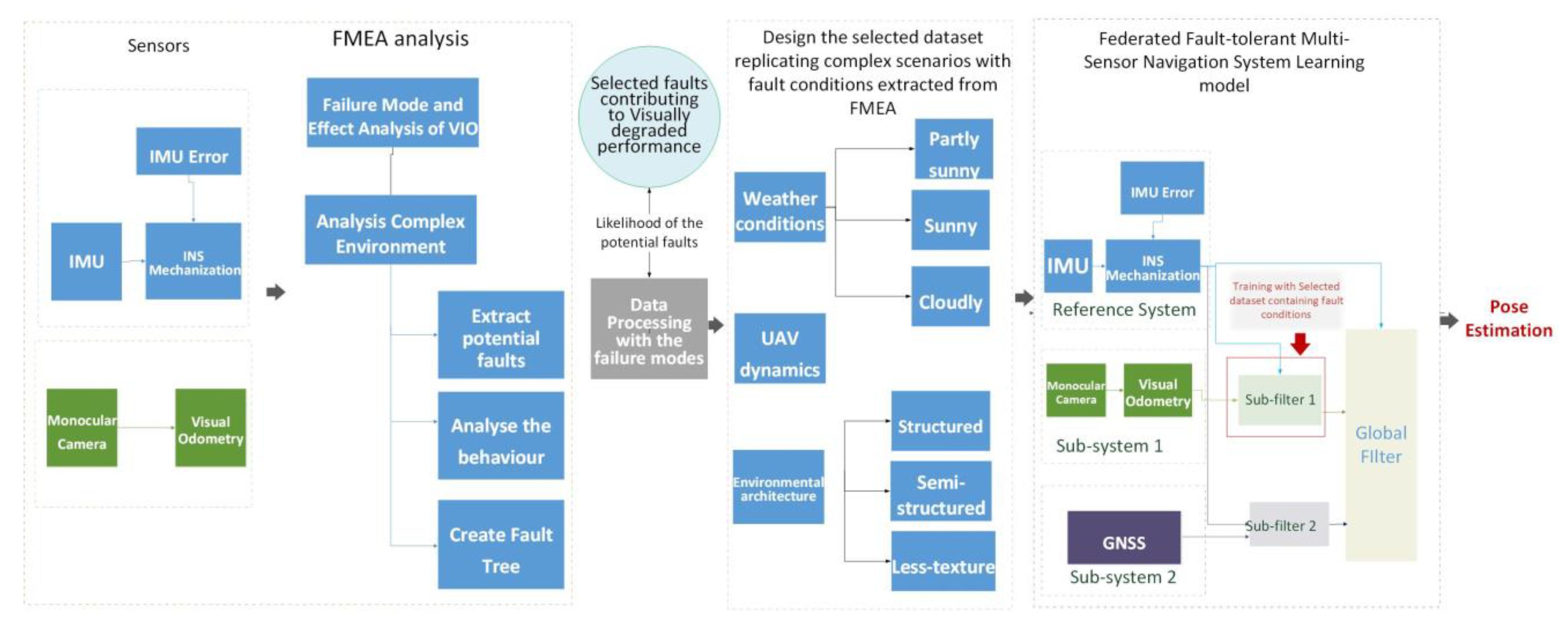
To correct visual positioning errors that arise from multiple systematic faults when navigating in urban areas, FMEA is executed at the first step to identify and analyse systematic failure modes according to the extracted fault tree model. The failure modes are prioritized based on potential impact and likelihood of occurrence, enabling the anticipation and mitigation of visual positioning errors. With the FMEA outcome, the hybrid GRU-aided ESKF VIO algorithm is discussed, as well as the algorithm implementation following the federated multi-sensor framework. The overall fault-tolerant multi-sensor system aided with FMEA is shown in Figure 2.

Figure 2. Fault-tolerant multi-sensor aided with FMEA framework.

3.1. Failure Mode and Effect Analysis (FMEA)

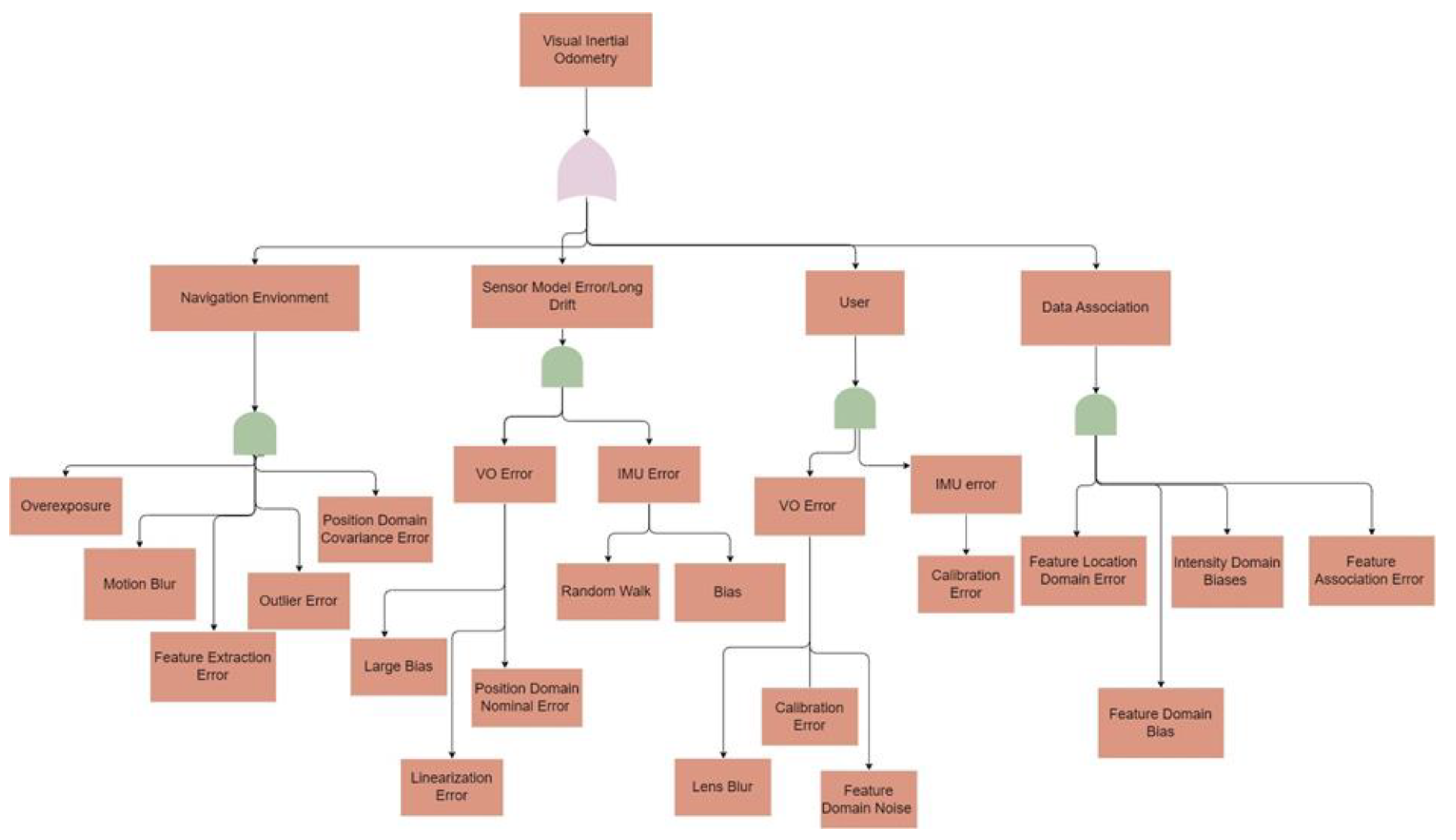
The implementation of FMEA on vision-based navigation systems enables the breaking down of high-level failure events into lower-level events along with allocating risks. Referring to error sources in every domain from the literature review [10], the fault tree model shown in Figure 3 is extracted.

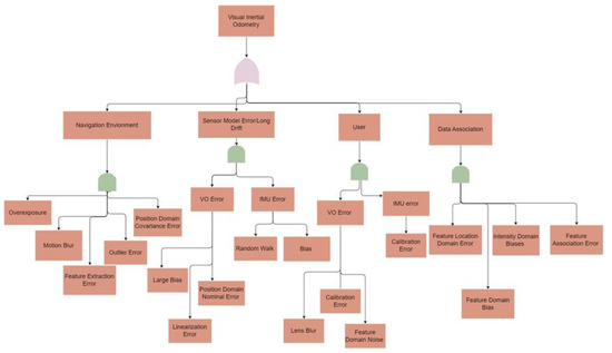
Figure 3. Fault tree analysis for feature-based VIO.

The preliminary conclusion of FMEA is that the error occultation in the camera presents a higher likelihood of the possibility during feature extraction due to the presence of multiple faults resulting in position errors in the whole system. Specifically, two major fault events, i.e., navigation environment errors and data association errors [10], show higher possibilities of faults in visual systems. Table 1 lists reviews of common error sources over the navigation environment and data association error events, along with their visual faults targeted for mitigation in the context of VIO.

Table 1. Common faults in the visual positioning based on a state-of-the-art review.

Error Sources	Fault Event	References	Error Effect
Feature Tracking Error	Navigation environment error	[45]	Motion blur
Outlier Error		[52]	Overexposure
		[12,45]	Rapid Motion
Feature Extraction Error		[10,12]	Overshoot
Feature Mismatch	Data Association error
Feature Domain Bias		[52]	Lighting Variation

• One common fault in the navigation environment fault event is the feature extraction error that contains deterministic biases that frequently lead to position errors.
• Another common fault in the data association failure event is the feature association error that occurs during matching 2D feature locations with 3D landmarks.
• The sensor model error/long drift failure events represent errors generated by sensor dynamics, including VO error and IMU error types.
• User failure events stand for the errors created during user operations that are normally relevant to the user calibration mistakes.

With the extension of fault events from the state-of-the-art reviews and proposition of thorough error analysis, i.e., Figure 3, this study aims to mitigate feature extraction errors occurring in failure modes linked to navigation environment and data association events through a fault-tolerant GNSS/IMU/VO navigation system. The hybrid integration of VIO holds great potential for achieving precise and reliable navigation performance in complex conditions.

3.2. Fault-Tolerant Federated Navigation System Architecture

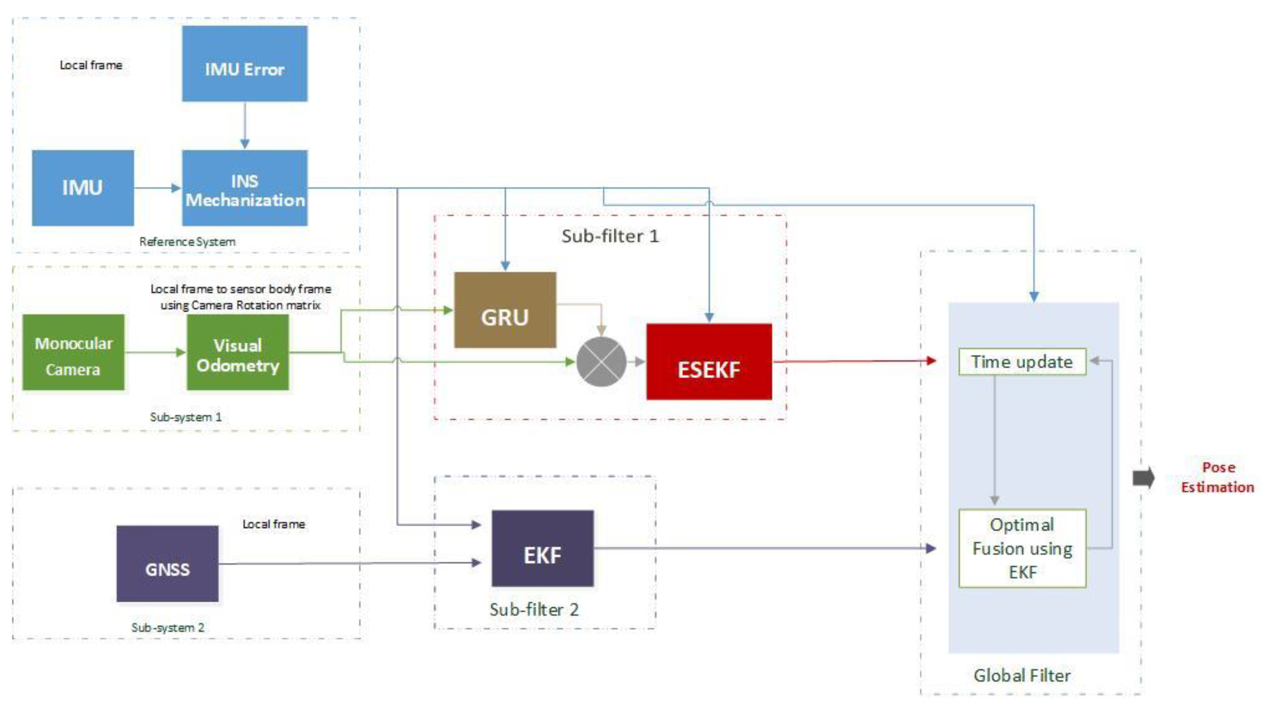
The utilization of a federated architecture proves advantageous in implementing fault-tolerant multi-sensor systems, as it is known for its robustness in handling faults. This paper proposes a federated architecture-based integrated multi-sensor fusion scheme based on the IMU, VO, and GNSS combination. The overall architecture of our method is shown in Figure 4.

Figure 4. The architecture of the proposed federated fault-tolerant multi-sensor navigation system.

Two sub-filters exist in the proposed architecture: a hybrid GRU-aided ESKF IMU/VO sub-filter and an EKF-based traditional GNSS/IMU integration sub-filter. The output of the two sub-filters is merged together with a global EKF to generate the ultimate position estimations. The former sub-filter of the hybrid GRU-aided ESKF IMU/VO attempts to compensate for VO errors, while the latter sub-filter of EKF-based GNSS/IMU integration aims to correct errors from GNSS and IMU.

3.2.1. Proposed GRU-aided ESKF VIO Integration (Sub-Filter 1)

ESKF VIO Fusion

In the tightly coupled GRU-aided ESKF VIO integration, pose measurements generated by VO are fused with the linear acceleration generated by the accelerometer and angular velocity generated by the gyroscope. The extraction of visual features by VO is firstly adapted to produce relative pose measurements for ESKF updates [14]. The system filter uses GRU-predicted VO increments to correct the corresponding VIO states to obtain the corrected position.

The state vector x of the proposed GRU-aided ESKF VIO selects the following states:

$$x=\left. [P_x, P_y,P_z, V_x,V_y,V_z,A_x,A_y,A_z,\Delta {\alpha }_b{}_x,\Delta {\alpha }_b{}_y,\Delta {\alpha }_b{}_z,\Delta {\omega }_b{}_x,\Delta {\omega }_b{}_y,\Delta {\omega }_b{}_z\right]$$

(1)

where, $P_x, P_y$ and $P_z$ denote the position, $V_x,V_y$and $V_z$ denote velocity, $A_x,A_y$ and $A_z$ denote attitude, $\Delta {\alpha }_x,\Delta {\alpha }_y$ and $\Delta {\alpha }_z$ denote accelerometer bias and $,\Delta {\omega }_x,\Delta {\omega }_y$ and $,\Delta {\omega }_z$ denote gyroscope bias in the x-axis, y-axis and z-axis.

The widely used, tightly coupled VIO is based on a Kalman filter [14]-[25]. The system dynamic model and measurement model are:

$$x_k={ \mathsf{\Sigma }}_k{x}_{k-1}+Q_k$$

(2)

$$z_k=H_k{x}_k+{\mathsf{\Pi }}_k$$

(3)

where $x_k$ and $x_{k-1}$ represent the system vector at $k$ and $k-1$ epoch; ${\mathsf{\Sigma }}_k$ and $Q_k$ represent the state transition matrix and system processing noise; $z_k$ and $H_k$ represent the measurement vector and measurement matrix; and ${\mathsf{\Pi }}_k$ represents the measurement noise.

Differing from conventional KF, ESKF uses an error-state representation, which has several benefits in terms of computational efficiency, numerical stability and prevention of singularities or gimbal lock issues. The details of the nominal and error states are included in the state-of-the-art research [14].

In order to improve positioning in diverse visual conditions, the predicted error measurements $P_{VO/GRU}$ are added to the error-state in a measurement update of ESKF. After the error-state update, the nominal state is updated with corrected error-states using the appropriate compositions:

$$x_k=x_{k-1}\oplus {\widehat{\partial X}}_k$$

(4)

In addition, the updated estimated state vector by correcting error states are:

$${\widehat{P}}_k={\widehat{P}}_{k|k-1}+{\widehat{\partial P}}_k+\Delta P_{VO|k-1}$$

(5)

$${\widehat{V}}_k={\widehat{V}}_{k|k-1}+{\widehat{\partial V}}_k$$

(6)

$${\widehat{A}}_k={\widehat{A}}_{k|k-1}+{\widehat{\partial A}}_k$$

(7)

$${\widehat{\alpha }}_k={\widehat{\alpha }}_{k|k-1}+\widehat{\partial {\alpha }_k}$$

(8)

$${\widehat{\omega }}_k={\widehat{\omega }}_{k|k-1}+{\widehat{\partial \omega }}_k$$

(9)

where, ${\widehat{P}}_k$ and ${\widehat{P}}_{k|k-1}$denote the nominal position vector at $k$ and $k-1$ epoch; ${\widehat{\partial P}}_k$ denotes the measured error-state position; $\Delta P_{VO|k-1}$ denotes the VO predicted increments vector at $k-1$ epoch; ${\widehat{V}}_k$ and ${\widehat{V}}_{k|k-1}$ denote the nominal velocity at $k$ and $k-1$; ${\widehat{\partial V}}_k$ denotes the measured error-state velocity; ${\widehat{A}}_k$ and ${\widehat{A}}_{k|k-1}$ denote the nominal attitude at $k$ and $k-1$; ${\widehat{\partial A}}_k$ denotes measured error-state attitude; ${\widehat{\alpha }}_k$ and ${\widehat{\alpha }}_{k|k-1}$ denote nominal acceleration bias at $k$ and $k-1$; ${\widehat{\partial \alpha }}_k$ denotes the measured error-state acceleration bias; ${\widehat{\omega }}_k$ and ${\widehat{\omega }}_{k|k-1}$ denote the nominal gyroscope bias at $k$ and $k-1$; and ${\widehat{\partial \omega }}_k$ denotes measured error-state gyroscope bias. After the error integrates into the updated nominal state, the error-state variables need to reset, which has been adopted from Zhonghan et al. [67].

The proposed VIO measurement update process is illustrated in the following equations:

$$K_k={ \hat{\mathsf{\Sigma }}}_{k|k-1}{H}_k{}^T{\left(H_k{ \hat{\mathsf{\Sigma }}}_{k|k-1}{H}_k{}^T+\mathsf{\Pi }\right)}^{-1}$$

(10)

$$x_k=x_{k|k-1}+K_k\left(z_k-H_k{\mathrm{x}}_{k|k-1}\right)$$

(11)

$${\mathsf{\Sigma }}_k=\left(1-K_k{H}_k\right){\mathsf{\Sigma }}_{k|k-1}$$

(12)

where $K_k$ represents Kalman gain, ${\mathsf{\Sigma }}_k$and ${ \hat{\mathsf{\Sigma }}}_{k|k-1}$ represent the measurement covariance matrix at $k$ and $k-1$ epoch.

GRU-Aided VIO

The VIO sub-filter uses the proposed ESKF-based tightly coupled integration strategy with a GRU model, which works during GNSS outages. The GRU consists of an update gate $z_t$ that controls the extent of the impact on the current state force by the previous state and a reset gate to determine the forgetfulness degree of the hidden state information $h_t$. The details of the GRU propagation formula and architecture are adapted from Geragersian et al. [68]. The formula for the GRU architecture is presented below:

$$z_t=\sigma \left(W^z{X}_t+U^z{h}_{t-1}\right)$$

(13)

$$r_t=\sigma \left(W^r{X}_t+U^r{h}_{t-1}\right)$$

(14)

here, $W^z$ and $W^r$ are the weight matrix of input for hidden layers and reset gate respectively; $U^z$ and $U^r$ are the weight matrix of the hidden state for hidden layers and reset gate, respectively; σ is the activation matrix.

The GRU model is trained with multiple trajectories containing complex scenarios that facilitate failure modes extracted using FMEA analysis so that it can predict VO error during flight under diverse conditions.

The GRU output equation is formulated by:

$$P_{VO/GRU}=P_{VO}-\Delta P_{VO}$$

(15)

where $P_{VO}$ denotes position error from VO, $\Delta P_{VO}$ is position error deviations, and $P_{VO/GRU}$ represents the predicted position increments.

The GRU model is shown in Figure 5.

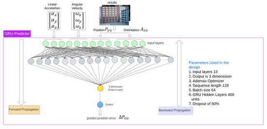
Figure 5. Illustrative diagram of GRU model.

Two data sources from IMU and VO are generated and used to gather positioning and attitude data for training each trajectory. Additionally, the VO position $P_{VO}$ and orientation ${\phi }_{VO}$ covering multiple complex environments by UAV and IMU measured angular velocity ${\alpha }_{INS}$ and linear acceleration ${\omega }_{INS}$are used to calculate inputs of GRU. The output of the GRU model is the positioning error $\Delta P_{VO}$generated by VO. When the GNSS signal is unavailable, IMU/VO operates to estimate the position of the UAV where the GRU module operates in predicting mode that predicts the position error $\Delta P_{VO}$, which is to be updated to the measurements vector in the ESKF module. When VO diverges, the GRU block predicts visual errors for error correction.

3.2.2. EKF Based GNSS/IMU Integration (Sub-Filter 2)

The tightly coupled architecture is implemented in the GNSS/MU integrated sub-filter of the proposed fault-tolerant multi-sensor navigation system. The GPS measurement position and IMU measurement acceleration and angular velocity proceed to estimate the state vector, including position velocity and attitude, using traditional EKF-based fusion filtering. Optimal states of the state vector from traditional EKF can be obtained through prediction and observation update and is discussed in Mitchel et al. [69]. The generic observation equation for EKF can be written as:

$$z_k{}_{GNSS/IMU}=H_k{}_{GNSS/IMU}{X}_k{}_{GNSS/IMU}+{\mathsf{\Lambda }}_{GNSS/IMU}$$

(16)

where, $H_k{}_{GNSS/IMU}$ represents the observation matrix; $z_k{}_{GNSS/IMU}$ represents the observation vector; $X_k{}_{GNSS/IMU}$ represents the observation state vector, and ${\mathsf{\Lambda }}_{GNSS/IMU}$ represents the observation noise matrix.

3.2.3. Federated Filter for Multi-Sensor Fusion

The proposed federated GNSS/IMU/VO multi-sensor navigation system uses VIO and GNSS/IMU integrated systems as the switching criterion. However, the global filter integration was conducted using the EKF approach to fuse the data generated by sub-filters. The detailed description and the state equations are the same as in the GNSS/INS sub-filter. In order to reduce computational complexity, the state equation of the GNSS/IMU sub-filter is the same as the global filter. The fusion resolution of the federated filter is as follows:

$$P_{k|global}={\displaystyle \sum }_{i=1}^r{P}_{il}$$

(17)

$$X_{k|global}=P_{k|global}{}^{-1}\left({\displaystyle \sum }_{i=1}^r{P}_{il}{X}_{il}\right)$$

(18)

where r is the number of sub-filters; $P_{k|global}$ and $P_{il}$ are the covariance vector of the ith sub-filter and the global filter; and $X_{k|global}$and $X_{il}$are the estimated states of ith sub-filter and the global filter. The global state estimation and the covariance vector are obtained by fusing the sub-filter estimated position, thus yielding a global solution.

The pseudo-code of the proposed fault-tolerant federated multi-sensor navigation system algorithm is presented in Algorithm 1.

Algorithm 1: Algorithm of GNSS/IMU/VO Multi-Sensor Navigation System

Input: $P_{VO}, {\alpha }_{xyz}, {\omega }_{xyz}, P_{GNSS}$//$P_{VO}$ denotes the VO estimated position; ${\alpha }_{xyz}$denotes the linear acceleration; ${\omega }_{xyz}$denotes the angular velocity; and $P_{GNSS}$ denotes the GNSS estimated position Output: $P_{VIO}, P_{GNSS/IMU}, P_{GNSS/IMU/VO}$ //$P_{VIO}$ denotes the sub-filter 1 estimated position; $P_{GNSS/IMU}$ denotes the sub-filter 2 estimated position; $\mathrm{and} P_{GNSS/IMU/VO}$ denotes the global filter estimated position Initialize: 1. $\mathrm{Initial} \mathrm{the} \mathrm{values} \mathrm{for} \mathrm{VIO} \mathrm{and} \mathrm{GNSS}/\mathrm{IMU} \mathrm{sub}-\mathrm{filters}: x_k=x_0$ ;//$x_0$denotes ground truth from UAV. 2. $\mathrm{Initial} \mathrm{values} \mathrm{for} \mathrm{global} \mathrm{filter} \mathrm{EKF}: x_{k|global}=x_0$;//$x_0$denotes the ground truth from UAV. for n = 1,2,3, …. do                    // n denotes number of iterations Prediction Phase: 3. The sub-filter time update model has been derived in Equation (2), which is similar for both sub-filters and global as using the EKF variant. 4. $\mathrm{Covariance} \mathrm{vector} \mathrm{is} \mathrm{defined} \mathrm{as}, {\mathsf{\Sigma }}_{k|k-1}=F_{k|k-1}{\mathsf{\Sigma }}_{k-1}{F}_{k|k-1}{}^T+L_{k|k-1}{Q}_{k-1}{L}_{k|k-1}{}^T$. Measurement Phase for sub-filters: 5. $\mathrm{Generate} \mathrm{the} P_{VO/GRU}$ predicted increments and updated the following measurement steps of the VIO sub-filter. 6. Estimate the states using the updated Equations (4)–(9). 7. Calculate the Kalman gain, updated VIO states, and the covariance matrix using Equations (10)–(12). 8. $\mathrm{Corrected} X_K{}_{VIO}=x_{k|k-1}{}_{VIO}+K_k{}_{VIO}\left(z_k{}_{VIO}-H_k{}_{VIO}{x}_{k|k-1}{}_{VIO}\right)$. 9. Start from step 7 to estimate the Kalman gain using Equation 10 for the GNSS/MU integration. 10. Update the observation Equation (16). 11. Estimate the updated states and covariance matrix of the GNSS/IMU filter using Equations (11) and (12). 12. The proposed VIO integrated sub-filter and GNSS/INS integration using EKF are running in parallel to estimate the position for each filter. Measurement update for Global filter: 13. Calculate the Kalman gain: $\hspace{1em}\hspace{1em}\hspace{1em}\hspace{1em}{K}_{global}={ \hat{\mathsf{\Sigma }}}_{global}{H}_k{{}_{global}}^T{\left(H_k{}_{global}{ \hat{\mathsf{\Sigma }}}_{k|k-1}{}_{global}{H}_k{{}_{global}}^T+{\mathsf{\Pi }}_{global}\right)}^{-1}$ 14. Update the states using the traditional EKF Equation (16). 15. $\mathrm{Obtain} P_{k|global}$ and $X_{k|global}$ using Equations (17) and (18). End for

4. Experimental Setup

To verify the proposed fault-tolerant navigation system performance under complex environments, a GNSS/IMU/VO simulator is built on Unreal Engine with UAV unity dynamic models integrated into urban scenarios in MATLAB 2022a. The sensors implemented in the simulator include an IMU block, GNSS receivers, and a front-facing monocular camera model generated by the Navigation Toolbox and UAV toolbox. The choice of a monocular camera is beneficial in our application due to its advantage of being less expensive, simpler to implement compared to a stereo camera, and lightweight to fit into a drone. The complex simulated environment is generated using Unreal Engine 5.0.3 and has a ‘US city’ scenario available in the ‘Simulation 3D Scene Configuration’ block. The simulated scenario used in the experiments is a bright sunny day with 20% floating clouds. The dataset is acquired with these sensors mounted on a quadrotor, as shown in Figure 6.

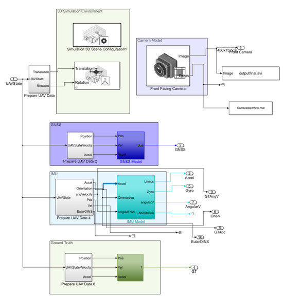
Figure 6. Experimental simulation setup in MATLAB.

The simulator consists of four blocks in total. The first block is the 3D simulation environment block, which aims to simulate the US city environment with a combination of camera- and UAV-based quadrotor models. The second block is GNSS integration with a quadrotor consisting of GNSS and the quadrotor dynamics. The third block is the IMU block interfaced with the quadrotor block. The fourth block is the ground truth from the quadrotor dynamics to provide true quadrotor trajectories.

The IMU selects the ICM 20649 model with the specifications provided in Table 2. The experimental data are collected with sampling rates of 10 Hz, 100 Hz, and 100 Hz for the camera, IMU, and GNSS, respectively. The random walk error [0.001, 0.001, 0.001] $m/s^2$ in the IMU accelerometer results in a position error growing at a quadratic rate.

Table 2. Specification of the ICM 20649 IMU model.

Parameter	Value
Accelerometer Bias Stability	$0.014 m/s^2$
Gyroscope Bias Stability	$0.0025 rad/s$
Angle Random Walk	$0.00043633 m/s^2\ast \surd Hz$
Velocity Random Walk	$0.0012356 m/s^2\ast \surd Hz$

The GNSS model is initialized by injecting two common failure modes of random walk and step error that will most likely occur in an urban environment, leading to a multipath effect.

The camera model has specifications, including a 1109 focal length, 640 × 360 optical center, and 720 × 1280 image size. Regarding the calibration of the camera and extraction of extrinsic and intrinsic parameters of the simulated front-facing camera, the coordinate conversion matrix from world coordination to pixel coordination is denoted by camera instincts matrix $k$:

$$k=\left. [\begin{array}{ccc}1109& 0& 640\\ 0& 1109& 360\\ 0& 0& 0\end{array}\right]$$

For urban operation scenarios surrounded by buildings, the visual data of tall buildings are captured by a camera for VIO to provide positioning information. Meanwhile, the satellite availability is obstructed by buildings, causing a GNSS outage. The MATLAB simulator connects to the QGroundControl software to generate real-time flight trajectories for the data collection and save it into text file format. The QGroundControl uses a MAVLink communicator to connect the base station of the UAV block in the Simulator [70]. The integration of MAVLink with MATLAB/Simulink is adopted into the UAV package delivery example.

Regarding the training GRU models, 10 trajectories covering more than 100,000 samples from each sensor are used for training. The sensor blocks, including IMU, the GPS provided by the UAV Toolbox, and the Navigation Toolbox, operate in the local frame. To ensure compatibility and effective data fusion using the proposed algorithm, a crucial step in the data pre-processing phase involves converting the data from the local frame to the sensor body frame. This transformation is essential for aligning the sensor data with the algorithm’s requirements and the system’s operational frame reference.

The general performance evaluation method uses root mean square error (RMSE) formulated by:

$$RMSE{ }_{overall}={\displaystyle \sum }_N^{i=1}\sqrt{\frac{{\left({(P_x{}_{Pre}-P_x{}_{GT})}^2+{(P_y{}_{Pre}-P_y{}_{GT})}^2+{(P_z{}_{Pre}-P_z{}_{GT})}^2\right)}^2}{N}}$$

(19)

here, $P_{xPre}, P_{yPre},P_{zPre},$are the predicted position generated by proposed algorithm in x-, y- and z-axis, respectively; $P_{xGT}, P_{yGT},P_{zGT}$ are the ground truth generated from UAV in x-, y- and z-axis, respectively. The number of samples is represented using capital N.

5. Test and Results

In order to evaluate the performance of the proposed GRU-aided ESKF-based VIO, two trajectories corresponding to experiments 1 and 2 are selected from the package delivery experiment in an urban environment. Both experiments are carried out under sunlight conditions, introducing common fault scenario shadows, lighting variations, motion blur, no-texture, and motion variation consistently present throughout the flight duration. For both experiments, a consistent fault condition is injected, i.e., the shadow of tall buildings on a sunny day during the fight. According to the fault types and number, the flying regions in the experiments are categorized into four distinct zones that encompass single faults, multiple faults, and combined faults. The faults arising from environmental sensitivity and dynamic motion transitions under previously estimated two major failure events in visual systems using FMEA analysis results in Section 3.1 have been discussed.

5.1. Experiment 1—Dense Urban Cynon

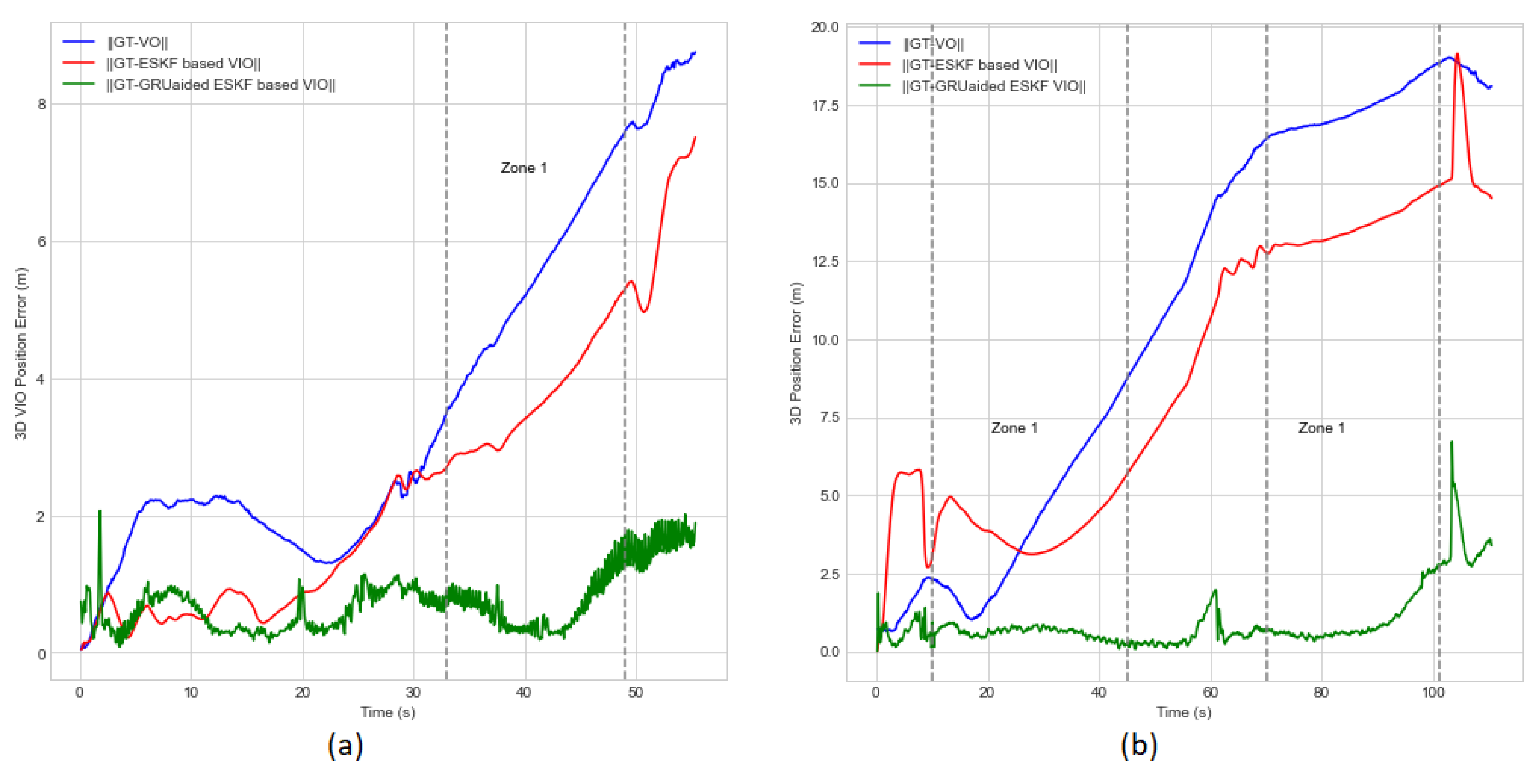
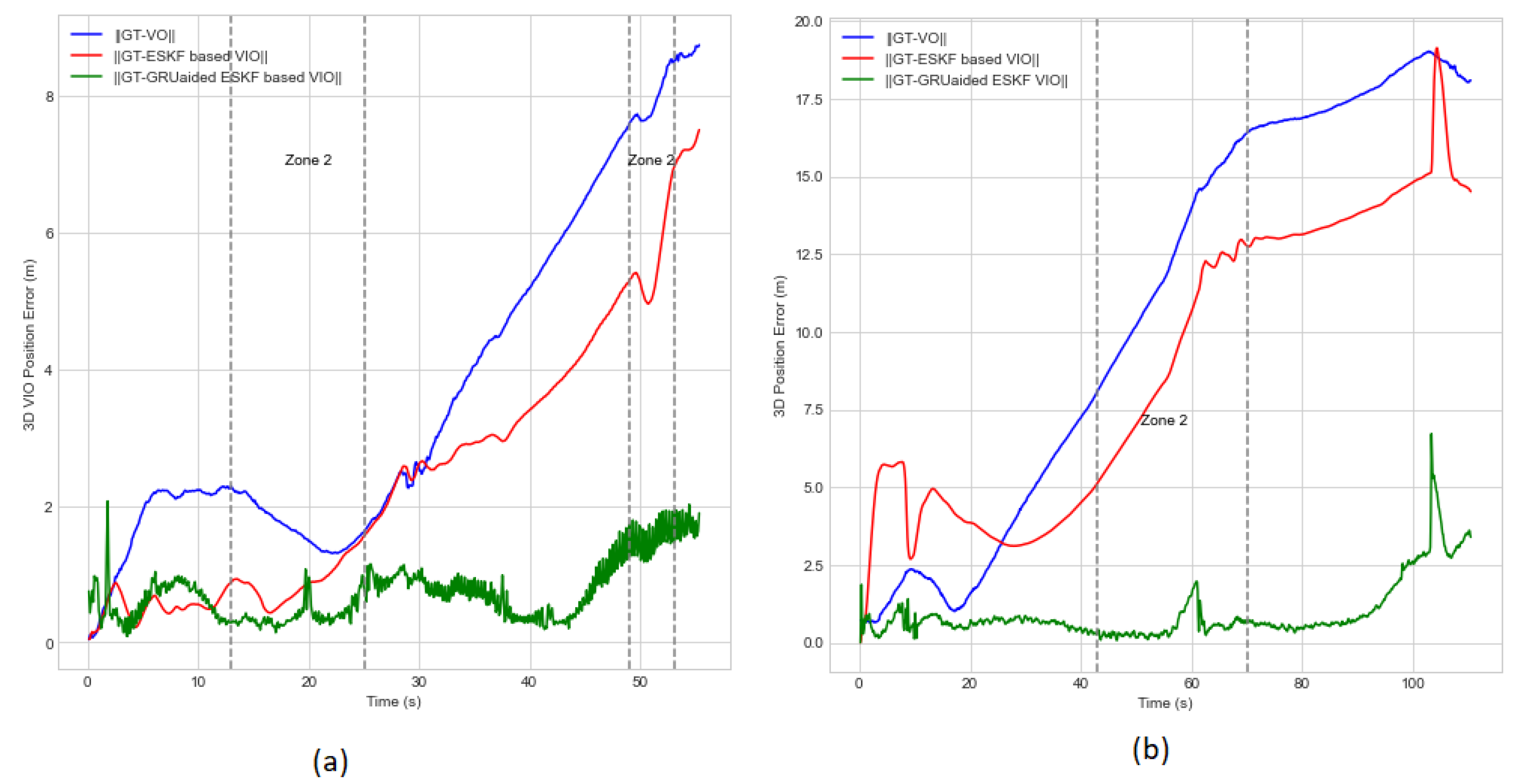
The purpose of this experiment is to validate the effectiveness of the proposed GRU-aided VIO in managing specific failure modes in complex conditions. This experimental environment includes a combination of tall and short buildings. During the experiment, a distance of 235 m was covered within a time span of 55 s. Figure 7 shows the accumulated 3D visual position error. Our proposed GRU-aided VIO is able to reduce position error by 86.6% compared with an ESKF-based VIO reference system. The maximum error in Figure 7 reduces from 7.5 m to 1.9 m with the GRU adoption.

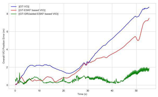
Figure 7. Overall visual navigation error in the presence of multiple failure modes for Experiment 1.

When the UAV takes off with rapid and sudden changes in waypoints, the Dynamic Motion Transitions failure mode occurs under the condition of jerking movements that consistently result in feature tracking errors and feature association error failure modes in VO. Moreover, the other dynamic motion transition failure mode is incorporated, i.e., turning to replicate complex environmental conditions, thereby emulating real fight scenarios. The UAV takes off speed sets to 20 m/s while its speed will increase up to 50 m/s at 7 s.

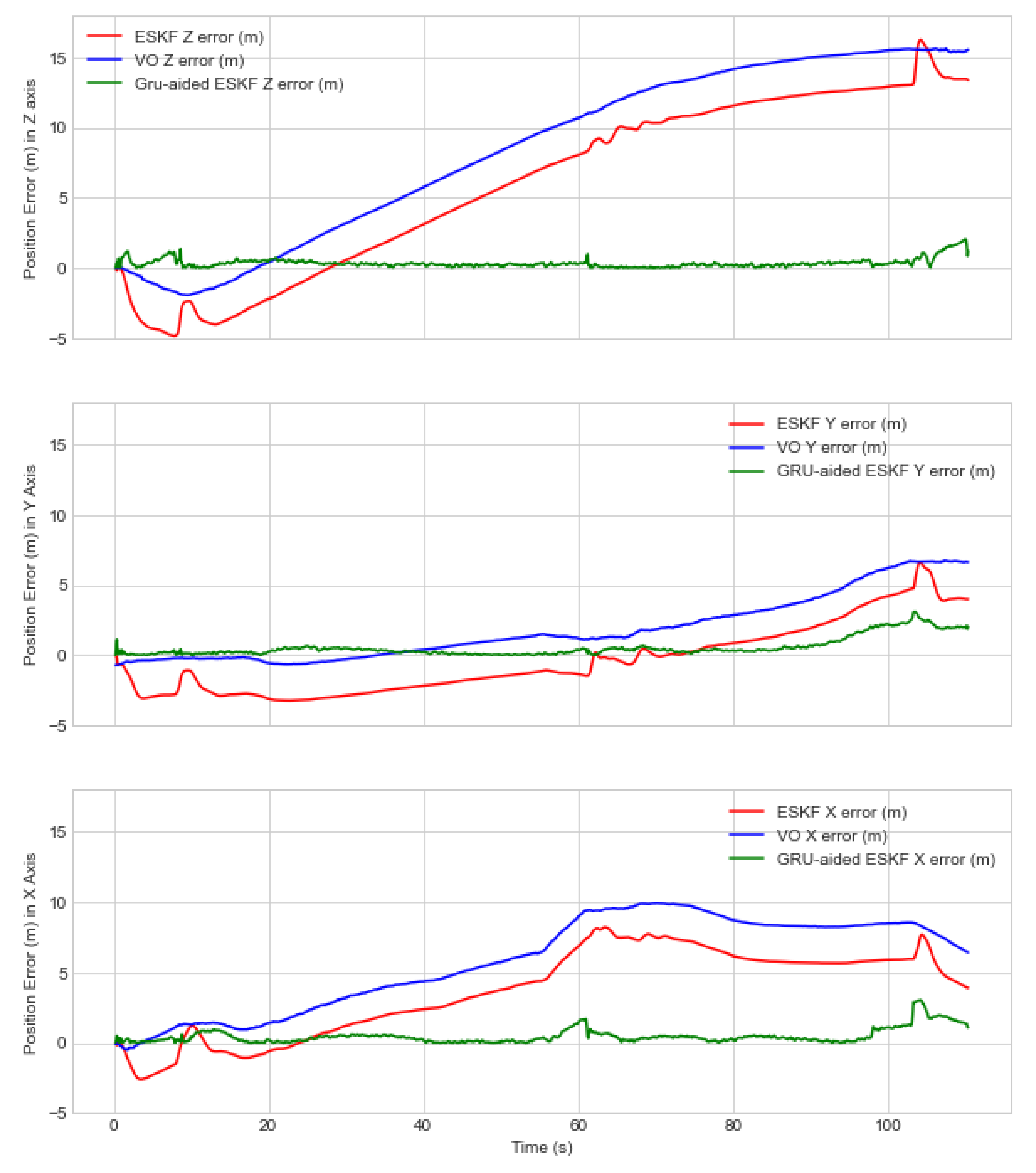
Figure 8 shows the RMSE position error of the proposed GRU-aided VIO system and benchmarked with two references of VO- and ESK-based VIO position error. The RMSE position error in the x-axis under NED coordination is relatively lower compared to y- and z-axis. It is worth noting that the maximum position error of the ESKF-based VIO reference system is 3.227 m, 5.6 m, and 4.1 m in the x, y, and z-axes.

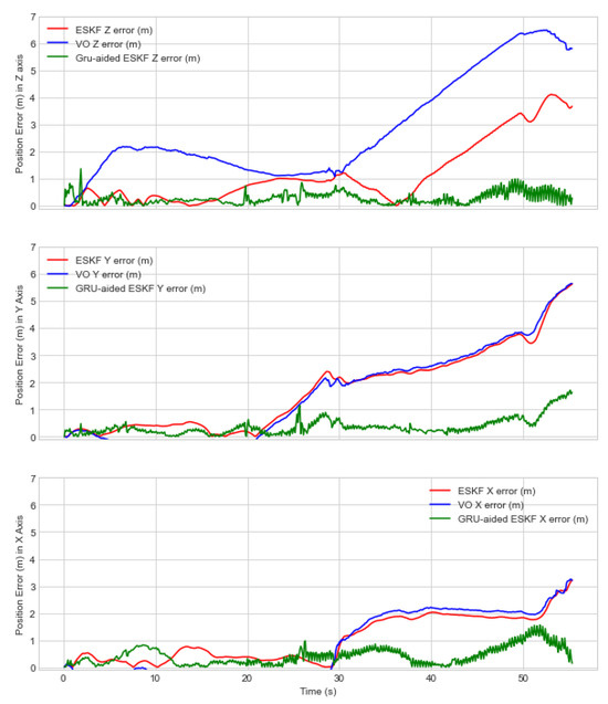
Figure 8. Visual navigation error along each axis in the presence of multiple failure modes for Experiment 1.

In the y-axis, the position error axis increases at 22 s due to the shadow of another building creating a variation of light. At 27 s, the UAV encounters a turn facing a plain wall because of a lack of textures, leading to drift, inaccuracies and failure of visual odometry. ESKF-based VIO showed relatively poor performance along the y-axis during diagonal motion due to cross-axis coupling and multiple failure modes due to featureless plain wall, sunlight variation, and shadow of tall buildings leading to feature degradation and tracking features. The loss of visual features results in insufficient information for ESKF to estimate the position accurately. In Figure 7 and Figure 8, it is shown that VIO based on ESKF fails to mitigate visual positioning error due to non-linear motion, lack of observable features, non-Gaussian noise, and uncertain state estimation, leading to non-linearization error propagation. However, it was found that our proposed solution can mitigate position error by 60.44%, 78.13% and 77.13% in the x-, y- and z-axes, respectively. The maximum position error is decreased from 1.5 m, 1.6 m, and 1.2 m.

When analyzing the z-axis performance in Figure 8, at around 37 s, the ESKF-based VIO position error starts increasing due to a dark wall shadowed from another tall building, causing variation of light in the frame leading to feature association error. ESKF performance degrades due to multiple factors present in the scenario, and error accumulates over time. After applying our proposed GRU-aided ESKF, the VIO fusion method is able to reduce position error at 37 s from 2.1 m to 0.6 m by predicting the VO error indicated with details in Table 3.

Table 3. RMSE Comparison on the performance of two experiments.

Experiment	Method	RMSE(m)-x-axis	RMSE(m)-y-axis	RMSE(m)-z-axis	RMSE(m)-Overall
1	VO	1.4	2.3	3.4	4.3
	ESKF VIO	1.3	2.2	1.6	3.1
	GRU-aided ESKF VIO	0.5	0.4	0.3	0.7
2	VO	6.6	2.9	10.4	12.6
	ESKF VIO	4.7	2.5	8.6	10.1
	GRU-aided ESKF VIO	0.8	0.9	0.5	1.3

5.2. Experiment 2—Semi-Structured Urban Environment

This experiment aims to measure GRU-aided ESKF VIO performance under environments of tall buildings with open space parking areas. In this experiment, the UAV encounters two turns, which means changing two waypoints at 60 s and 110 s, leading to motion variation causing feature association error described as ‘Dynamic Motion Transitions’.

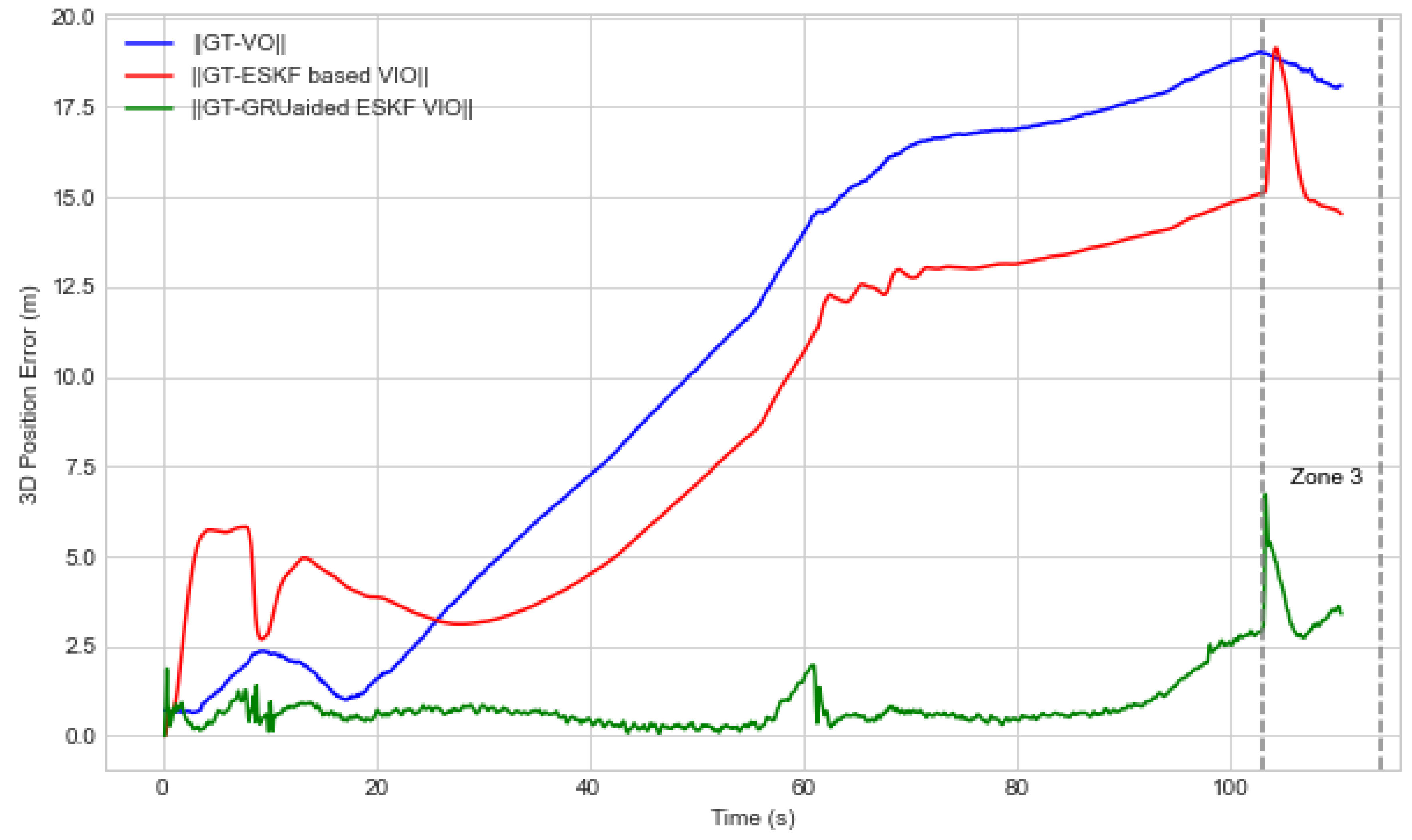
Figure 9 shows the accumulated 3D position error of the proposed GRU-aided ESKF VIO system and is benchmarked with two references of VO- and ESKF-based VIO position error. In Figure 9, the position error in the first few seconds is negative due to multiple factors, such as shadows of tall buildings, trees on plain surfaces, shadowed buildings, and lighting variations due to sunlight, motion blur, and rapid motion. The maximum position error is 19.1 m at 110 s due to combinational failure modes such as dark wall, rapid motion and motion blur. The proposed GRU-aided ESKF VIO is able to mitigate 86.62% of overall position error. The maximum error is reduced from 19.1 m to 6.8 m.

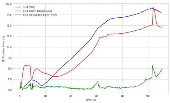
Figure 9. The D-position error in the presence of multiple failure modes for Experiment 2.

Figure 10 shows the VIO position RMSE error in the separate x-, y- and z-axes. Table 3 indicates that position error RMSE of ESKF is 4.7 m, 2.5 m, and 8.6 m in the x-, y- and z-axes, respectively. The proposed GRU-aided ESKF VIO has a remarkable improvement in terms of position error, and the specific values along the x-, y- and z-axes are 0.8 m, 0.9 m, and 0.5 m, respectively. Due to cross-axis coupling, the y-axis faces a larger estimated position error than others. During the time interval of 57–65 s, UAV takes a turn and passes through a parking area where buildings are under limited field of view. In this case, the feature extraction and tracing processes encounter challenges and lead to position estimation errors. The proposed solution has shown excellent performance improvement in the presence of failure modes of feature extraction error and feature tracking error, where the position error is decreased by 62.86% in comparison to the reference systems.

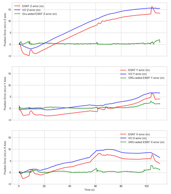
Figure 10. Position error along each axis in the presence of multiple failure modes for Experiment 2.

When analysing the z-axis performance in Figure 10, the proposed GRU-aided ESKF VIO outperforms the reference ESKF fusion with respect to a reduction in the z-axis error by 93.46%. According to Table 3, the reference ESKF has shown the worst performance of 8.6 m RMSE compared to the proposed method of 0.5 m RMSE. It is noted that at 104 s during the landing phase, the UAV turns around and encounters a black wall. This leads to higher performance errors because the VO system struggles to extract enough features in the complex scene with poor lighting [6,8,9]. The GRU-aided ESKF VIO demonstrates improvement compared to the traditional ESKF-based approach, resulting in a remarkable reduction of error of 93.45%. The maximum position error in the z-axis due to dark scene at 110 s is reduced from 16.2 m to 3.0 m. During the experiment, a distance of 459 m was covered within a time span of 1 min 50 s.

Table 4 indicates the maximum position error comparison for two of the experiments. By integrating fault-tolerant mechanisms, our approach achieves more accurate position estimation, even in challenging situations with limited visual cues. The fault-tolerant GRU-aided ESKF VIO architecture shows robustness over a number of realistic visual degradation scenarios.

Table 4. Maximum position error comparison for two experiments.

Experiment	Method	Maximum Error in x-axis (m)-	Maximum Error in y-axis (m)-	Maximum Error in z-axis (m)-	Maximum 3D Error (m)-
	ESKF VIO	3.2	5.6	4.1	7.5
1	GRU-aided ESKF VIO	1.5	1.6	1.2	1.9
	ESKF VIO	8.2	6.6	16.2	19.1
2	GRU-aided ESKF VIO	5.0	4.4	3.0	6.8

5.3. Performance Evaluation Based on Zone Categories

To further evaluate the successful rate when mitigating failure modes from experiments 1 and 2, as detailed in Section 3.1, the fault zones are extracted in the above two experiments.

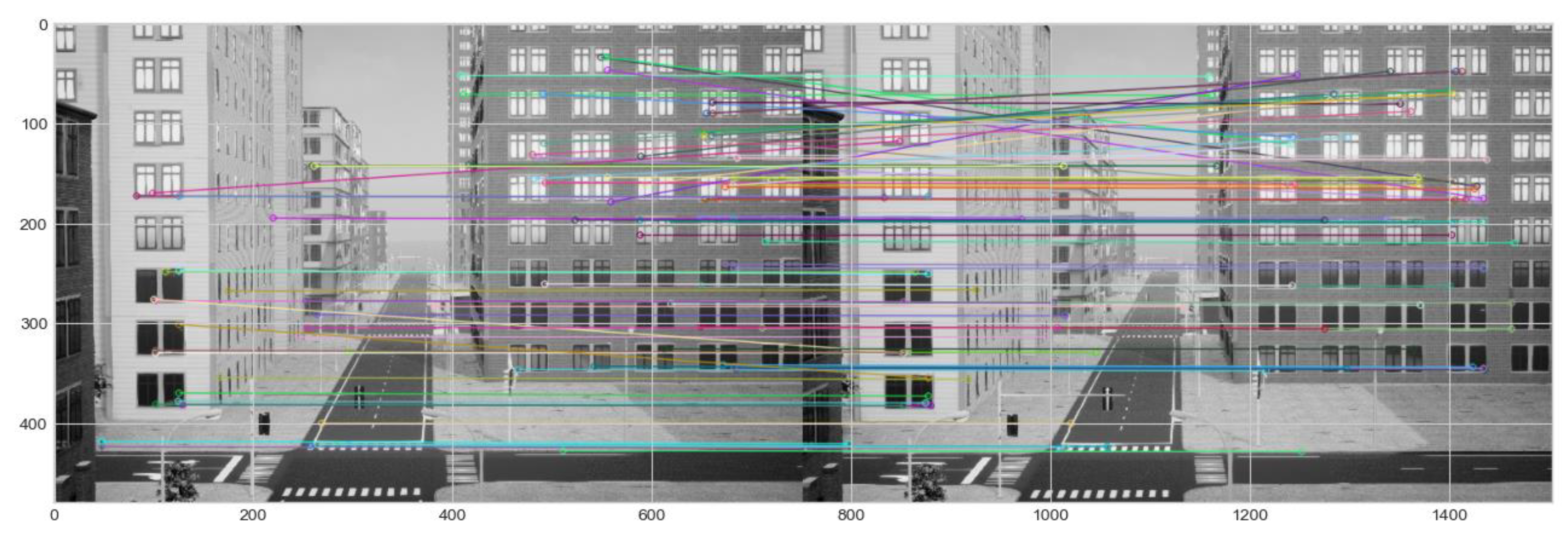
Zone 1 indicates building shadow as the single fault triggering feature matching and feature tracking error failure modes within the time interval. In experiment 1, between the time interval of 33–49 s, UAV passes through shadow buildings that distort visual features, causing incorrect matches and tracking errors when they move into or out of shadows, as shown in Figure 11. In addition, introducing the sudden change in lighting may be misinterpreted as IMU acceleration and rotation.

Figure 11. Feature tracking and Feature mismatch error failure modes due to tall-shadowed buildings in experiment 1.

Figure 12 a,b depict the zone 1 region to show performance comparisons of our proposed algorithm with the reference algorithms in the presence of two failure modes. The maximum position errors for experiment 1 in zone 1 along x-, y- and z-axes are reduced by 52.38%, 81.57%, and 73.17%, respectively. In experiment 2, a single fault is encountered twice during the time interval of 13–44 s and 70–106 s. Maximum position error in the time interval of 13–44 s in x-, y- and z-axes are reduced by 93.33%, 75%, and 85%, respectively. Hence, the proposed solution proves to be robust over two failure modes.

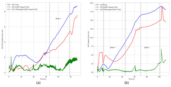
Figure 12. Position errors of Zone 1 (shadowed building) estimated in each axis for experiment 1 (a). Position errors of Zone 1 (shadowed building) estimated in each axis for experiment 2 (b).

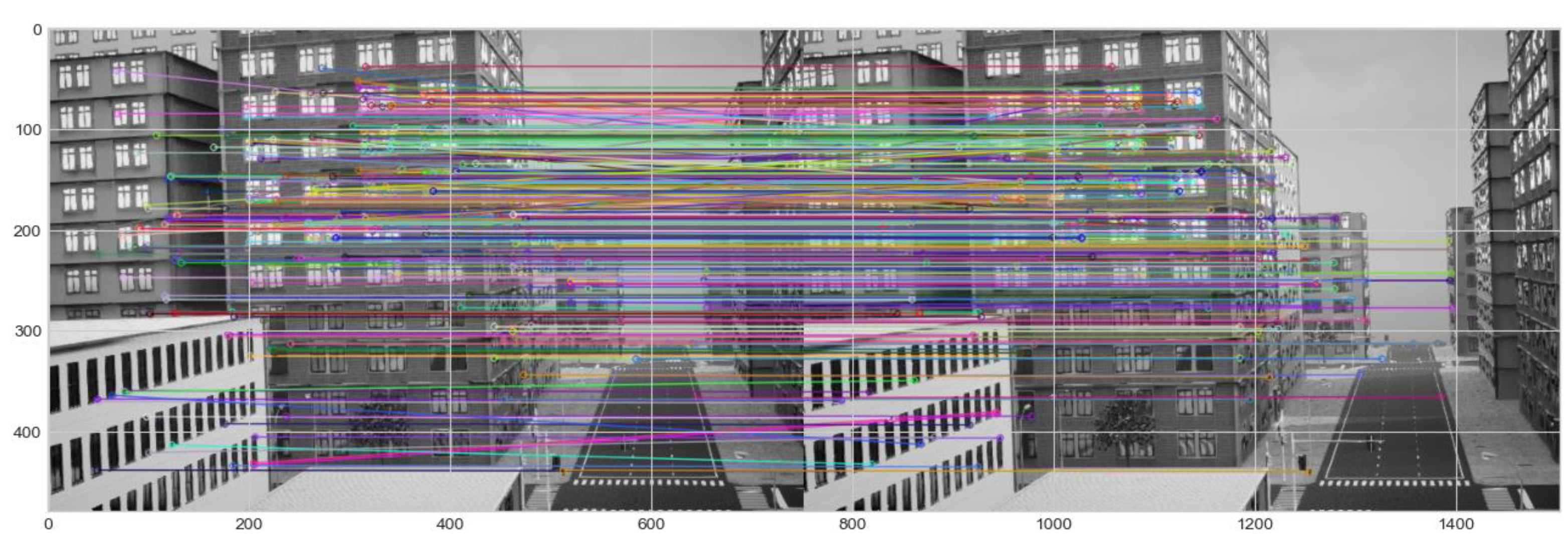
Zone 2 includes multiple faults, including turning manoeuvre and shadow of tall buildings that are present in both experiments. When a UAV makes a turn, the motion dynamics change rapidly. This leads to challenges in estimating camera motion and orientation estimations, causing tracking errors. In the meantime, visual distortion also causes feature extraction errors and feature mismatch errors due to inconsistent lighting, as shown in Figure 13. The combination of both conditions adds complexity to the environment, exacerbating the existing challenges in traditional ESKF-based VIO. Our proposed algorithm is able to mitigate these failure modes and shows robustness in such complex scenes compared with traditional VIO systems. The algorithm is able to mitigate motion dynamics and feature extraction error, reducing feature matching error by 20%, 20%, and 50% at the time interval of 13–24 s in experiment 1 and 62.5%, 40%, and 90% at the time interval of 45–70 s with respect to the x-, y- and z-axes, as shown in Figure 14a,b.

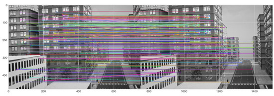
Figure 13. Motion dynamics, feature tracking and feature mismatch error failure modes due to the tall, shadowed buildings in experiment 2.

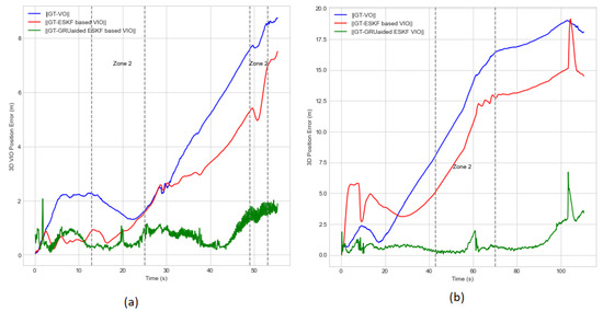
Figure 14. Position errors of Zone 2 (shadowed building and UAV turns) estimated in each axis for experiment 1 (a). Position errors of Zone 2 (shadowed building and UAV turn) estimated in each axis for experiment 2 (b).

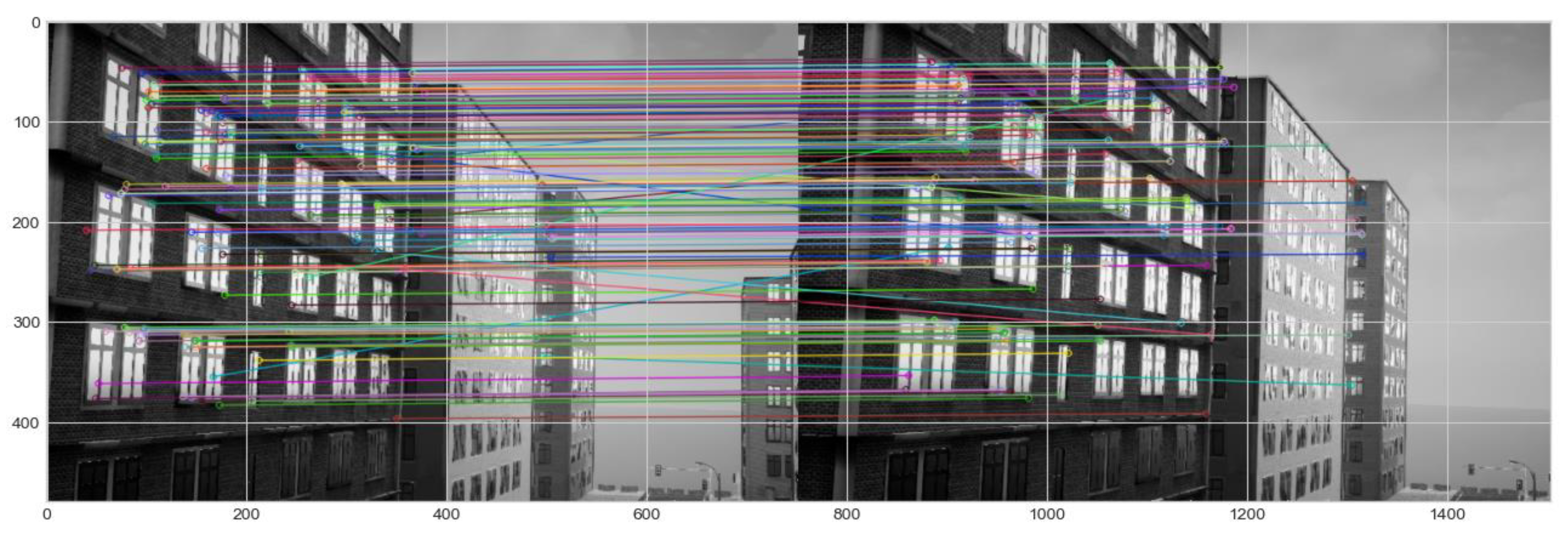
In Zone 3, multiple faults are combined together, including the turning manoeuvre, shadows from the tall buildings, variations in lighting, areas of darkness and sunlight shadows. Zone 3 only exists as one of the most complex conditions in experiment 2. As observed in Zone 1 and Zone 2, the turning behaviour and shadow of the tall buildings introduce changes in motion dynamics that make the position estimation and feature tracking challenging for traditional, ESKF-based VIO. Additionally, the presence of both dark and well-lit areas within the scene created abrupt changes in illumination.

Figure 15 presents one demonstration image from the mounted front-facing camera in a UAV when passing through an illuminated and shaded area. The shadows caused by direct sunlight also create sharp pixel contrast between illuminated and shaded areas. These sudden lighting changes and the combination of multiple fault conditions amplify the challenges posed by each individual fault, making the overall VIO performance more susceptible to tracking errors, feature mismatches, and feature extraction error failure modes.

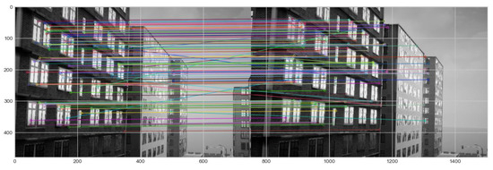
Figure 15. Feature tracking, feature extraction error, and feature mismatch failure modes for dark and well-illuminated tall buildings in experiment 2.

Figure 16 shows that the GRU-aided ESKF VIO architecture reduces maximum position error in experiment 2 at the time interval of 107–114 s from 32.6%, 81.327%, and 64.397% in x-, y- and z-axes. Therefore, the GRU-aided fusion algorithm can perform without interruption when the UAV navigates in illuminated and shaded areas and has shown robustness in the presence of multiple failure modes and moving features amidst dynamic lighting.

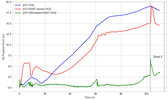
Figure 16. Position errors in Zone 3 (UAV turn and illuminated tall buildings) estimated in each axis for experiment 2.

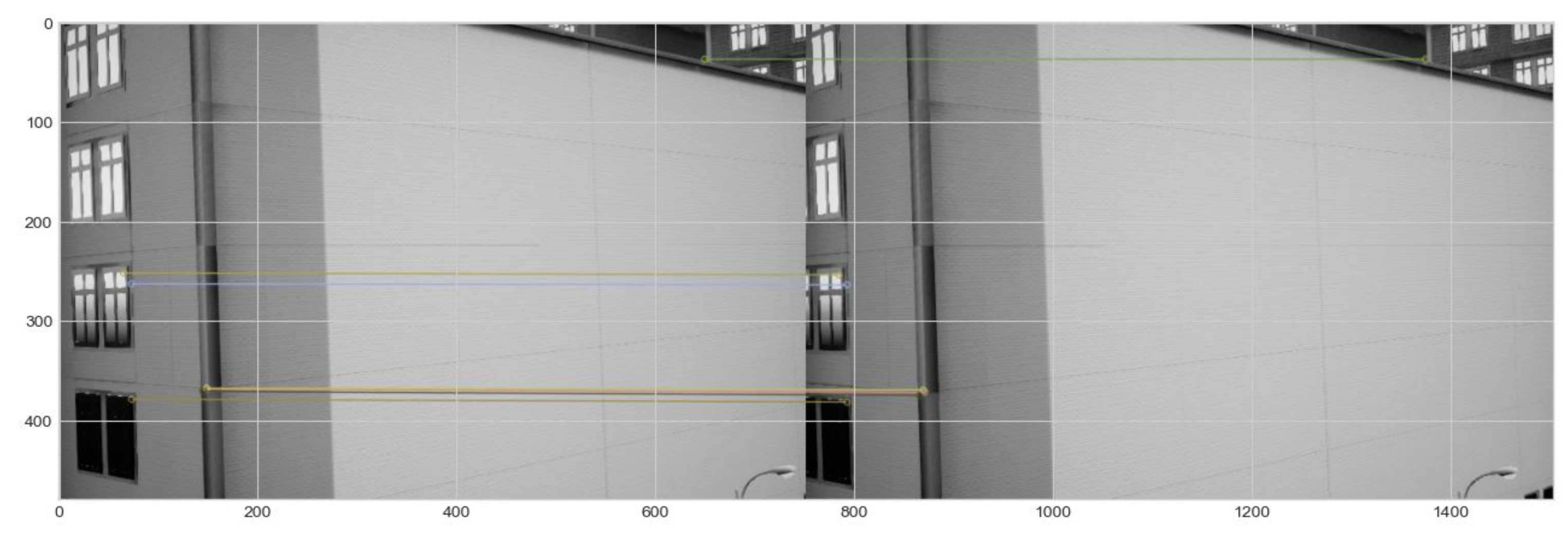
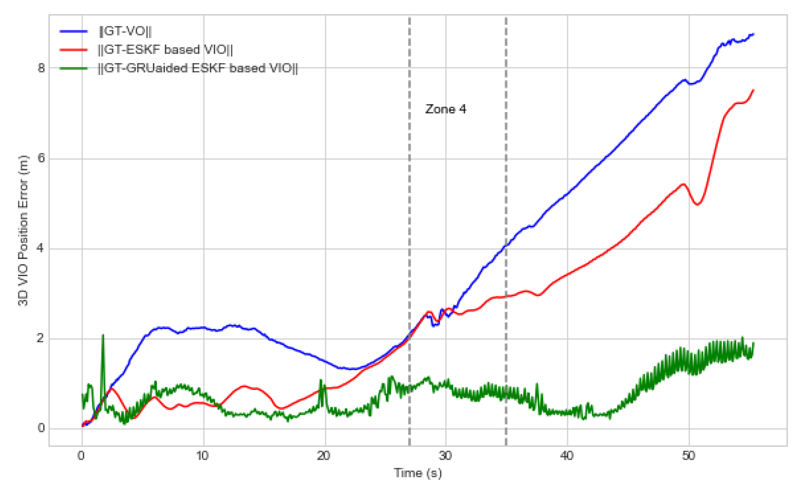
Zone 4 consists of a combination of complex faults, including navigation environmental error and data association fault events. The fault events consist of turning manoeuvres, building shadows, the presence of featureless blank walls and variation in lighting. In experiment 1, the UAV encountered a plain wall at 27–32 s of its flight, resulting in a feature extraction error due to the lack of distinctive features on the wall shown in Figure 17. As a result, the feature extraction process failed, leading to a lack of identifiable features to track and match in consecutive frames. Such lack of features caused the VO to lose its frame-to-frame correspondence, resulting in the inability to accurately estimate the UAV’s motion in this specific time of 27–32 s. Figure 18 shows the increment of position error caused by the mentioned disruption. The ESKF algorithm performance is heavily affected, leading to incremental tracking errors and loss of tracking when dealing with a featureless wall. Figure 18 shows that our algorithm has effectively reduced the maximum position error by 42.1%, 63.3%, and 60.12% in x-, y- and z-axes, respectively.

Figure 17. Feature extraction error due to the plain wall in experiment 1.

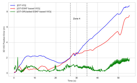
Figure 18. Position errors of Zone 4 (UAV turn, shadowed buildings, and featureless wall buildings) estimated in each axis for experiment 1.

To evaluate the performance of the proposed fault-tolerant federated multi-sensor navigation system, the experiment is conducted using the Experiment 1 dataset with GNSS condition applied (faulted-GNSS and without fault GNSS) adopted from [71]. Table 5 shows the performance comparison results of the proposed GRU-aided ESKF VIO with faulted GNSS and no-fault GNSS. The results indicate that the hybrid approach enables mitigating the overall position error even with faulted GNSS conditions compared to [11,71]. Therefore, it is approved that the FMEA-assisted fault-tolerant multi-sensor navigation system facilitates positioning performance in the presence of multiple faults covering all the sensor faults in diverse, complex environments.

Table 5. The RMSE of 3D position errors of GNSS/faulted-IMU/faulted-VO solution with faulted-GNSS/faulted-IMU/faulted-VO.

Algorithms	3D RMSE Position Error (m)
Faulted-VO/GNSS/IMU	1.2
Faulted-VIO-ESKF/GNSS/IMU	0.7
Faulted-GRU-aided-ESKF-VIO/GNSS/IMU	0.09
Faulted-VO/Faulted-GNSS/IMU	1.5
Faulted-ESKF-VIO/Faulted-GNSS/IMU	1.0
Faulted-GRU-aided-ESKF-VIO/Faulted-GNSS/IMU	0.2

5.4. Performance Comparison with Other Datasets

This paper selects the EUROC dataset, specifically MH05_difficult, for benchmarking with other algorithms since EUROC is commonly applied by other researchers [12,45]. The EUROC sequence dataset was collected in an indoor machine hall with light variation. MH05_difficult dataset contained black and white images, which they referred to as dark and shadowed environments and captured with rapid motion. The dataset is captured in a customized way that has several limitations, including manipulated images, customized blur, and brightness.

Figure 19 presents the 3D position error of running our proposed GRU-aided ESKF VIO to process MH05_difficult. The key finding is that the position error in RMSE is reduced by 67.32%. The maximum error is reduced from 2.81 m to 1.5 m.

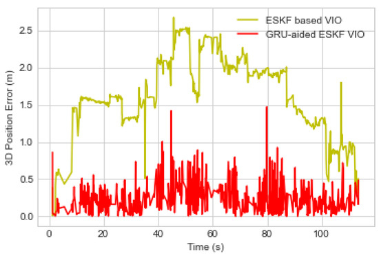
Figure 19. The D position error estimated using a MH05 seq EUROC Dataset with a motion blur failure mode.

Table 6 highlights the comparison results in terms of the accumulated RSME with state-of-the-art systems, i.e., End-to-End VIO, Self-supervised VIO [12,45]. It is worth mentioning that the EUROC dataset does not provide tight synchronization between IMU and images, which is a primary requirement of using RNN-based VIO.

Table 6. Comparison with state-of-the-art methods that used MH_05 seq. EUROC Dataset with motion blur failure mode.

Algorithms	RMSE (m)-of MH_05 seq	Improvement
End-to-end VIO [45]	1.96 m	66.32%
Self-supervised VIO [12]	1.48 m	55.4%%
Proposed GRU-aided ESKF VIO	0.66 m	---------

By cross-checking with the work of Brandon et al. [12], the proposed GRU-aided ESKF VIO confirms the robust improvement in the presence of motion blur failure mode.

6. Conclusions

Aiming to provide fault-tolerant VIO navigation solutions against complex environments, this study proposed a hybrid federated navigation system framework aided by FMEA for enabling fault tolerance and GRU fused with ESKF-VIO to mitigate visual positioning errors.

Through simulations, the main advantages of the GRU and ESKF hybrid algorithm are summarized as follows: (1) A high-efficiency recurrent neural cell with simple architecture, namely the GRU, was chosen to predict the position error during visual degradation. Benefiting from the proper selection of the Kalman filter performance enhancement method, such as updating the state vector by predicting errors using the AI method, our proposed algorithm possesses superior navigation accuracy under complex conditions. (2) The FMEA analysis helps to prioritize anticipated failure modes such as feature extraction error, feature tracking error, and motion dynamics, enabling us to mitigate position error caused by these failure modes before they lead to operation failure. (3) The mitigation of feature extraction failure modes, which can subsequently lead to feature association errors. Via demonstrations, it is found that multiple factors or faults within the navigation environment and the UAV’s dynamics reduce the impact of those failures.

This approach represents a significant step towards improving the robustness and reliability of VIO, particularly in complex and dynamic environments where feature extraction error, feature tracking error, and feature mismatch are critical for accurate navigation. With the correction of the VIO, the fault-tolerant multi-sensor performance is demonstrated to be improved under diverse, complex urban environments in terms of robustness and accuracy at different time scales, enabling uninterrupted and seamless flight operations.

References

- Arafat, M.Y.; Alam, M.M.; Moh, S. Vision-Based Navigation Techniques for Unmanned Aerial Vehicles: Review and Challenges. Drones 2023, 7, 89. [Google Scholar] [CrossRef]
- Alkendi, Y.; Seneviratne, L.; Zweiri, Y. State of the Art in Vision-Based Localization Techniques for Autonomous Navigation Systems. IEEE Access 2021, 9, 76847–76874. [Google Scholar] [CrossRef]
- Afia, A.B.; Escher, A.; Macabiau, C. A Low-cost GNSS/IMU/Visual monoSLAM/WSS Integration Based on Federated Kalman Filtering for Navigation in Urban Environments. In Proceedings of the 28th International Technical Meeting of the Satellite Division of The Institute of Navigation (ION GNSS+ 2015), Tampa, FL, USA, 14–18 September 2015. [Google Scholar]
- Lee, Y.D.; Kim, L.W.; Lee, H.K. A tightly-coupled compressed-state constraint Kalman Filter for integrated visual-inertial-Global Navigation Satellite System navigation in GNSS-Degraded environments. IET Radar Sonar Navig. 2022, 16, 1344–1363. [Google Scholar] [CrossRef]
- Liao, J.; Li, X.; Wang, X.; Li, S.; Wang, H. Enhancing navigation performance through visual-inertial odometry in GNSS-degraded environment. GPS Solut. 2021, 25, 50. [Google Scholar] [CrossRef]
- Qin, T.; Li, P.; Shen, S. VINS-Mono: A Robust and Versatile Monocular Visual-Inertial State Estimator. IEEE Trans. Robot. 2018, 34, 1004–1020. [Google Scholar] [CrossRef]
- Mourikis, A.I.; Roumeliotis, S.I. A multi-state constraint Kalman filter for vision-aided inertial navigation. In Proceedings of the Proceedings 2007 IEEE International Conference on Robotics and Automation, Rome, Italy, 10–14 April 2007; pp. 3565–3572. [Google Scholar] [CrossRef]
- Campos, C.; Elvira, R.; Rodriguez, J.J.G.; Montiel, J.M.M.; Tardos, J.D. ORB-SLAM3: An Accurate Open-Source Library for Visual, Visual-Inertial, and Multimap SLAM. IEEE Trans. Robot. 2021, 37, 1874–1890. [Google Scholar] [CrossRef]
- Geneva, P.; Eckenhoff, K.; Lee, W.; Yang, Y.; Huang, G. OpenVINS: A Research Platform for Visual-Inertial Estimation. In Proceedings of the 2020 IEEE International Conference on Robotics and Automation (ICRA), Paris, France, 31 May–31 August 2020; pp. 4666–4672. [Google Scholar] [CrossRef]
- Zhu, C.; Meurer, M.; Günther, C. Integrity of Visual Navigation—Developments, Challenges, and Prospects. Navig. J. Inst. Navig. 2022, 69, 518. [Google Scholar] [CrossRef]
- JDai, J.; Hao, X.; Liu, S.; Ren, Z. Research on UAV Robust Adaptive Positioning Algorithm Based on IMU/GNSS/VO in Complex Scenes. Sensors 2022, 22, 2832. [Google Scholar] [CrossRef]
- Wagstaff, B.; Wise, E.; Kelly, J. A Self-Supervised, Differentiable Kalman Filter for Uncertainty-Aware Visual-Inertial Odometry. In Proceedings of the IEEE/ASME International Conference on Advanced Intelligent Mechatronics, AIM, Sapporo, Japan, 11–15 July 2022; pp. 1388–1395. [Google Scholar] [CrossRef]
- Zhai, Y.; Fu, Y.; Wang, S.; Zhan, X. Mechanism Analysis and Mitigation of Visual Navigation System Vulnerability. In China Satellite Navigation Conference (CSNC 2021) Proceedings; Springer: Singapore, 2021; Volume 773, pp. 515–524. [Google Scholar] [CrossRef]
- Markovic, L.; Kovac, M.; Milijas, R.; Car, M.; Bogdan, S. Error State Extended Kalman Filter Multi-Sensor Fusion for Unmanned Aerial Vehicle Localization in GPS and Magnetometer Denied Indoor Environments. In Proceedings of the 2022 International Conference on Unmanned Aircraft Systems, ICUAS 2022, Dubrovnik, Croatia, 21–24 June 2022; pp. 184–190. [Google Scholar] [CrossRef]
- Xiong, X.; Chen, W.; Liu, Z.; Shen, Q. DS-VIO: Robust and Efficient Stereo Visual Inertial Odometry based on Dual Stage EKF. arXiv 2019, arXiv:1905.00684. [Google Scholar]
- Fanin, F.; Hong, J.H. Visual Inertial Navigation for a Small UAV Using Sparse and Dense Optical Flow. In Proceedings of the 2019 Workshop on Research, Education and Development of Unmanned Aerial Systems (RED UAS), Cranfield, UK, 25–27 November 2019. [Google Scholar]
- Bloesch, M.; Burri, M.; Omari, S.; Hutter, M.; Siegwart, R. Iterated extended Kalman filter based visual-inertial odometry using direct photometric feedback. Int. J. Robot. Res. 2017, 36, 1053–1072. [Google Scholar] [CrossRef]
- Sun, K.; Mohta, K.; Pfrommer, B.; Watterson, M.; Liu, S.; Mulgaonkar, Y.; Taylor, C.J.; Kumar, V. Robust Stereo Visual Inertial Odometry for Fast Autonomous Flight. IEEE Robot. Autom. Lett. 2018, 3, 965–972. [Google Scholar] [CrossRef]
- Li, G.; Yu, L.; Fei, S. A Binocular MSCKF-Based Visual Inertial Odometry System Using LK Optical Flow. J. Intell. Robot. Syst. Theory Appl. 2020, 100, 1179–1194. [Google Scholar] [CrossRef]
- Yang, Y.; Geneva, P.; Eckenhoff, K.; Huang, G. Visual-Inertial Odometry with Point and Line Features. In Proceedings of the IEEE International Conference on Intelligent Robots and Systems, Macau, China, 3–8 November 2019; pp. 2447–2454. [Google Scholar] [CrossRef]
- Ma, F.; Shi, J.; Yang, Y.; Li, J.; Dai, K. ACK-MSCKF: Tightly-coupled ackermann multi-state constraint kalman filter for autonomous vehicle localization. Sensors 2019, 19, 4816. [Google Scholar] [CrossRef] [PubMed]
- Wang, Z.; Pang, B.; Song, Y.; Yuan, X.; Xu, Q.; Li, Y. Robust Visual-Inertial Odometry Based on a Kalman Filter and Factor Graph. IEEE Trans. Intell. Transp. Syst. 2023, 24, 7048–7060. [Google Scholar] [CrossRef]
- Omotuyi, O.; Kumar, M. UAV Visual-Inertial Dynamics (VI-D) Odometry using Unscented Kalman Filter. IFAC Pap. 2021, 54, 814–819. [Google Scholar] [CrossRef]
- Sang, X.; Li, J.; Yuan, Z.; Yu, X.; Zhang, J.; Zhang, J.; Yang, P. Invariant Cubature Kalman Filtering-Based Visual-Inertial Odometry for Robot Pose Estimation. IEEE Sensors J. 2022, 22, 23413–23422. [Google Scholar] [CrossRef]
- Xu, J.; Yu, H.; Teng, R. Visual-inertial odometry using iterated cubature Kalman filter. In Proceedings of the 30th Chinese Control and Decision Conference, CCDC, Shenyang, China, 9–11 June 2018; pp. 3837–3841. [Google Scholar] [CrossRef]
- Liu, Y.; Xiong, R.; Wang, Y.; Huang, H.; Xie, X.; Liu, X.; Zhang, G. Stereo Visual-Inertial Odometry with Multiple Kalman Filters Ensemble. IEEE Trans. Ind. Electron. 2016, 63, 6205–6216. [Google Scholar] [CrossRef]
- Kim, S.; Petrunin, I.; Shin, H.-S. A Review of Kalman Filter with Artificial Intelligence Techniques. In Proceedings of the Integrated Communications, Navigation and Surveillance Conference, ICNS, Dulles, VA, USA, 5–7 April 2022; Institute of Electrical and Electronics Engineers Inc.: Piscataway, NJ, USA, 2022. [Google Scholar] [CrossRef]
- Jwo, D.-J.; Biswal, A.; Mir, I.A. Artificial Neural Networks for Navigation Systems: A Review of Recent Research. Appl. Sci. 2023, 13, 4475. [Google Scholar] [CrossRef]
- Shaukat, N.; Ali, A.; Moinuddin, M.; Otero, P. Underwater Vehicle Localization by Hybridization of Indirect Kalman Filter and Neural Network. In Proceedings of the 2021 7th International Conference on Mechatronics and Robotics Engineering, ICMRE 2021, Budapest, Hungary, 3–5 February 2021; Institute of Electrical and Electronics Engineers Inc.: Piscataway, NJ, USA, 2021; pp. 111–115. [Google Scholar] [CrossRef]
- Shaukat, N.; Ali, A.; Iqbal, M.J.; Moinuddin, M.; Otero, P. Multi-sensor fusion for underwater vehicle localization by augmentation of rbf neural network and error-state kalman filter. Sensors 2021, 21, 1149. [Google Scholar] [CrossRef]
- Vargas-Meléndez, L.; Boada, B.L.; Boada, M.J.L.; Gauchía, A.; Díaz, V. A sensor fusion method based on an integrated neural network and Kalman Filter for vehicle roll angle estimation. Sensors 2016, 16, 1400. [Google Scholar] [CrossRef]
- Jingsen, Z.; Wenjie, Z.; Bo, H.; Yali, W. Integrating Extreme Learning Machine with Kalman Filter to Bridge GPS Outages. In Proceedings of the 2016 3rd International Conference on Information Science and Control Engineering, ICISCE 2016, Beijing, China, 8–10 July 2016; Institute of Electrical and Electronics Engineers Inc.: Piscataway, NJ, USA, 2016; pp. 420–424. [Google Scholar] [CrossRef]
- Zhang, X.; Mu, X.; Liu, H.; He, B.; Yan, T. Application of Modified EKF Based on Intelligent Data Fusion in AUV Navigation; Application of Modified EKF Based on Intelligent Data Fusion in AUV Navigation. In Proceedings of the 2019 IEEE Underwater Technology (UT), Kaohsiung, Taiwan, 16–19 April 2019. [Google Scholar]
- Al Bitar, N.; Gavrilov, A.I. Neural_Networks_Aided_Unscented_Kalman_Filter_for_Integrated_INS_GNSS_Systems. In Proceedings of the 27th Saint Petersburg International Conference on Integrated Navigation Systems (ICINS), St. Petersburg, Russia, 25–17 May 2020; pp. 1–4. [Google Scholar]
- Miljković, Z.; Vuković, N.; Mitić, M. Neural extended Kalman filter for monocular SLAM in indoor environment. Proc. Inst. Mech. Eng. C J. Mech. Eng. Sci. 2016, 230, 856–866. [Google Scholar] [CrossRef]
- Choi, M.; Sakthivel, R.; Chung, W.K. Neural Network-Aided Extended Kalman Filter for SLAM Problem. In Proceedings of the 2007 IEEE International Conference on Robotics and Automation, Rome, Italy, 10–14 April 2007; pp. 1686–1690. [Google Scholar]
- Kotov, K.Y.; Maltsev, A.S.; Sobolev, M.A. Recurrent neural network and extended Kalman filter in SLAM problem. IFAC Proc. Vol. 2013, 46, 23–26. [Google Scholar] [CrossRef]
- Chen, L.; Fang, J. A Hybrid Prediction Method for Bridging GPS Outages in High-Precision POS Application. IEEE Trans. Instrum. Meas. 2014, 63, 1656–1665. [Google Scholar] [CrossRef]
- Lee, J.K.; Jekeli, C. Neural Network Aided Adaptive Filtering and Smoothing for an Integrated INS/GPS Unexploded Ordnance Geolocation System. J. Navig. 2010, 63, 251–267. [Google Scholar] [CrossRef]
- Bi, S.; Ma, L.; Shen, T.; Xu, Y.; Li, F. Neural network assisted Kalman filter for INS/UWB integrated seamless quadrotor localization. PeerJ Comput. Sci. 2021, 7, e630. [Google Scholar] [CrossRef] [PubMed]
- Zhao, S.; Zhou, Y.; Huang, T. A Novel Method for AI-Assisted INS/GNSS Navigation System Based on CNN-GRU and CKF during GNSS Outage. Remote Sens. 2022, 14, 4494. [Google Scholar] [CrossRef]
- Xie, D.; Jiang, J.; Wu, J.; Yan, P.; Tang, Y.; Zhang, C.; Liu, J. A Robust GNSS/PDR Integration Scheme with GRU-Based Zero-Velocity Detection for Mass-Pedestrians. Remote Sens. 2022, 14, 300. [Google Scholar] [CrossRef]
- Jiang, Y.; Nong, X. A Radar Filtering Model for Aerial Surveillance Base on Kalman Filter and Neural Network. In Proceedings of the IEEE International Conference on Software Engineering and Service Sciences, ICSESS, Beijing, China, 16–18 October 2020; pp. 57–60. [Google Scholar] [CrossRef]
- Miao, Z.; Shi, H.; Zhang, Y.; Xu, F. Neural network-aided variational Bayesian adaptive cubature Kalman filtering for nonlinear state estimation. Meas. Sci. Technol. 2017, 28, 10500. [Google Scholar] [CrossRef]
- Li, C.; Waslander, S. Towards End-to-end Learning of Visual Inertial Odometry with an EKF. In Proceedings of the 2020 17th Conference on Computer and Robot Vision, CRV 2020, Ottawa, ON, Canada, 13–15 May 2020; pp. 190–197. [Google Scholar] [CrossRef]
- Tang, Y.; Jiang, J.; Liu, J.; Yan, P.; Tao, Y.; Liu, J. A GRU and AKF-Based Hybrid Algorithm for Improving INS/GNSS Navigation Accuracy during GNSS Outage. Remote Sens. 2022, 14, 752. [Google Scholar] [CrossRef]
- Hosseinyalamdary, S. Deep Kalman Filter: Simultaneous Multi-Sensor Integration and Modelling; A GNSS/IMU Case Study. Sensors 2018, 18, 1316. [Google Scholar] [CrossRef]
- Song, L.; Duan, Z.; He, B.; Li, Z. Application of Federal Kalman Filter with Neural Networks in the Velocity and Attitude Matching of Transfer Alignment. Complexity 2018, 2018, 3039061. [Google Scholar] [CrossRef]
- Li, D.; Wu, Y.; Zhao, J. Novel Hybrid Algorithm of Improved CKF and GRU for GPS/INS. IEEE Access 2020, 8, 202836–202847. [Google Scholar] [CrossRef]
- Gao, X.; Luo, H.; Ning, B.; Zhao, F.; Bao, L.; Gong, Y.; Xiao, Y.; Jiang, J. RL-AKF: An Adaptive Kalman Filter Navigation Algorithm Based on Reinforcement Learning for Ground Vehicles. Remote Sens. 2020, 12, 1704. [Google Scholar] [CrossRef]
- Aslan, M.F.; Durdu, A.; Sabanci, K. Visual-Inertial Image-Odometry Network (VIIONet): A Gaussian process regression-based deep architecture proposal for UAV pose estimation. Measurement 2022, 194, 111030. [Google Scholar] [CrossRef]
- Chen, C.; Lu, C.X.; Wang, B.; Trigoni, N.; Markham, A. DynaNet: Neural Kalman Dynamical Model for Motion Estimation and Prediction. IEEE Trans. Neural Networks Learn. Syst. 2021, 32, 5479–5491. [Google Scholar] [CrossRef] [PubMed]
- Yusefi, A.; Durdu, A.; Aslan, M.F.; Sungur, C. LSTM and Filter Based Comparison Analysis for Indoor Global Localization in UAVs. IEEE Access 2021, 9, 10054–10069. [Google Scholar] [CrossRef]
- Zuo, S.; Shen, K.; Zuo, J. Robust Visual-Inertial Odometry Based on Deep Learning and Extended Kalman Filter. In Proceedings of the 2021 China Automation Congress, CAC 2021, Beijing, China, 22–24 October 2021; pp. 1173–1178. [Google Scholar] [CrossRef]
- Luo, Y.; Hu, J.; Guo, C. Right Invariant SE2(3)—EKF for Relative Navigation in Learning-based Visual Inertial Odometry. In Proceedings of the 2022 5th International Symposium on Autonomous Systems, ISAS 2022, Hangzhou, China, 8–10 April 2022. [Google Scholar] [CrossRef]
- Bhatti, U.I.; Ochieng, W.Y. Failure Modes and Models for Integrated GPS/INS Systems. J. Navig. 2007, 60, 327–348. [Google Scholar] [CrossRef]
- YDu, Y.; Wang, J.; Rizos, C.; El-Mowafy, A. Vulnerabilities and integrity of precise point positioning for intelligent transport systems: Overview and analysis. Satell. Navig. 2021, 2, 3. [Google Scholar] [CrossRef]
- Burri, M.; Nikolic, J.; Gohl, P.; Schneider, T.; Rehder, J.; Omari, S.; Achtelik, M.W.; Siegwart, R. The EuRoC micro aerial vehicle datasets. Int. J. Robot. Res. 2016, 35, 1157–1163. [Google Scholar] [CrossRef]
- Gao, B.; Hu, G.; Zhong, Y.; Zhu, X. Cubature Kalman Filter With Both Adaptability and Robustness for Tightly-Coupled GNSS/INS Integration. IEEE Sensors J. 2021, 21, 14997–15011. [Google Scholar] [CrossRef]
- Gao, B.; Gao, S.; Zhong, Y.; Hu, G.; Gu, C. Interacting multiple model estimation-based adaptive robust unscented Kalman filter. Int. J. Control Autom. Syst. 2017, 15, 2013–2025. [Google Scholar] [CrossRef]
- Gao, G.; Zhong, Y.; Gao, S.; Gao, B. Double-Channel Sequential Probability Ratio Test for Failure Detection in Multisensor Integrated Systems. IEEE Trans. Instrum. Meas. 2021, 70, 1–14. [Google Scholar] [CrossRef]
- Gao, G.; Gao, B.; Gao, S.; Hu, G.; Zhong, Y. A Hypothesis Test-Constrained Robust Kalman Filter for INS/GNSS Integration With Abnormal Measurement. IEEE Trans. Veh. Technol. 2022, 72, 1662–1673. [Google Scholar] [CrossRef]
- Gao, B.; Li, W.; Hu, G.; Zhong, Y.; Zhu, X. Mahalanobis distance-based fading cubature Kalman filter with augmented mechanism for hypersonic vehicle INS/CNS autonomous integration. Chin. J. Aeronaut. 2022, 35, 114–128. [Google Scholar] [CrossRef]
- Gao, B.; Hu, G.; Zhong, Y.; Zhu, X. Cubature rule-based distributed optimal fusion with identification and prediction of kinematic model error for integrated UAV navigation. Aerosp. Sci. Technol. 2021, 109, 106447. [Google Scholar] [CrossRef]
- Gao, B.; Hu, G.; Zhu, X.; Zhong, Y. A Robust Cubature Kalman Filter with Abnormal Observations Identification Using the Mahalanobis Distance Criterion for Vehicular INS/GNSS Integration. Sensors 2019, 19, 5149. [Google Scholar] [CrossRef] [PubMed]
- Hu, G.; Gao, B.; Zhong, Y.; Ni, L.; Gu, C. Robust Unscented Kalman Filtering With Measurement Error Detection for Tightly Coupled INS/GNSS Integration in Hypersonic Vehicle Navigation. IEEE Access 2019, 7, 151409–151421. [Google Scholar] [CrossRef]
- Li, Z.; Zhang, Y. Constrained ESKF for UAV Positioning in Indoor Corridor Environment Based on IMU and WiFi. Sensors 2022, 22, 391. [Google Scholar] [CrossRef]
- Geragersian, P.; Petrunin, I.; Guo, W.; Grech, R. An INS/GNSS fusion architecture in GNSS denied environments using gated recurrent units. In Proceedings of the AIAA Science and Technology Forum and Exposition, AIAA SciTech Forum 2022, San Diego, CA, USA, 3–7 January 2022. [Google Scholar] [CrossRef]
- Kourabbaslou, S.S.; Zhang, A.; Atia, M.M. A Novel Design Framework for Tightly Coupled IMU/GNSS Sensor Fusion Using Inverse-Kinematics, Symbolic Engines, and Genetic Algorithms. IEEE Sens. J. 2019, 19, 11424–11436. [Google Scholar] [CrossRef]
- Ramirez-Atencia, C.; Camacho, D. Extending QGroundControl for Automated Mission Planning of UAVs. Sensors 2018, 18, 2339. [Google Scholar] [CrossRef]
- Hernandez, G.E.V.; Petrunin, I.; Shin, H.-S.; Gilmour, J. Robust multi-sensor navigation in GNSS degraded environments. In Proceedings of the AIAA SCITECH 2023 Forum, National Harbor, MD, USA, 23–27 January 2023. [Google Scholar] [CrossRef]
Disclaimer/Publisher’s Note: The statements, opinions and data contained in all publications are solely those of the individual author(s) and contributor(s) and not of MDPI and/or the editor(s). MDPI and/or the editor(s) disclaim responsibility for any injury to people or property resulting from any ideas, methods, instructions or products referred to in the content. |
© 2023 by the authors. Licensee MDPI, Basel, Switzerland. This article is an open access article distributed under the terms and conditions of the Creative Commons Attribution (CC BY) license (https://creativecommons.org/licenses/by/4.0/).