Abstract
Performing online damage evaluation of blades subjected to complex cyclic loads based on the operating state of a gas turbine enables real-time reflection of a blade’s damage condition. This, in turn, facilitates the achievement of predictive maintenance objectives, enhancing the economic and operational stability of gas turbine operations. This study establishes a hybrid model for online damage evaluation of gas turbine blades based on their operational state. The model comprises a gas turbine performance model based on thermodynamic simulation, a component load calculation model based on a surrogate model, an updated cycle counting method based on four-point rainflow, and an improved damage mechanism evaluation model. In the new model, the use of a surrogate model for the estimation of blade loading information based on gas turbine operating parameters replaces the conventional physical modeling methods. This substitution enhances the accuracy of blade loading calculations while ensuring real-time performance. Additionally, the new model introduces an updated cycle counting method based on four-point rainflow and an improved damage mechanism evaluation model. In the temperature counting part, a characteristic stress that represents the stress information during the cyclic process is proposed. This inclusion allows for the consideration of the impact of stress fluctuations on creep damage, thereby enhancing the accuracy of the fatigue damage assessment. In the stress counting part, the model incorporates time information associated with each cycle. This concept is subsequently applied in determining the identified cyclic strain information, thereby improving the accuracy of the fatigue damage evaluation. Finally, this study applies the new model to an online damage evaluation of a turbine stationary blade using actual operating data from a micro gas turbine. The results obtained from the new model are compared with the EOH recommended by the OEM, validating the accuracy and applicability of the new model.
1. Introduction
Gas turbines possess significant advantages such as high energy efficiency, strong fuel adaptability, and low emissions of pollutants, making them advanced power equipment for constructing a clean, low-carbon, safe, and efficient energy system. As one of the most critical and complex components in gas turbines, the lifetime of blades directly impacts the economic viability and stability of gas turbine operations [1]. The lifetime of blades is closely related to the operational mode of gas turbines, the health status of various components, the maintenance history, and other factors. Neglecting the impact of these factors in the evaluation of blade lifetime can lead to the blade being out of repair and ultimately result in severe operational accidents [2]. Real-time monitoring of blade lifetime degradation, the fatigue–creep damage state, and providing appropriate maintenance recommendations based on the evaluation results are crucial for the continuous safe operation of gas turbines. In recent years, there has been increasing attention on online monitoring and the remaining useful life prediction of gas turbine blades based on operational conditions [3,4,5].
The method of damage evaluation based on operational conditions requires continuous evaluation of the damage state of components based on real-time load information. This involves utilizing sensor-measured parameters to monitor the stress and temperature information of components under current operating conditions in gas turbines. By efficiently processing real-time load data and incorporating different damage mechanisms, a precise damage evaluation can be conducted. The existing evaluation methods can be mainly classified into three categories: data-driven models, physical models, and hybrid models [6]. Data-driven models establish specific relationships between state parameters and variables of interest by utilizing a large amount of historical operational data. S. Yang and X. Jiang [7] used data-driven methods such as probabilistic statistics, signal processing, and artificial intelligence to predict the remaining useful life of components based on equipment operating conditions. This approach reduces the complexity associated with physically analyzing and modeling the components. However, pure data-driven methods face fundamental challenges in providing interpretable, reliable, and practical solutions due to limitations in data availability, the black-box nature of machine learning, and the diversity of operational conditions [8]. Physical models are mathematical descriptions or simulation models constructed based on the physical principles and fundamental laws of a system. D. Zhou and colleagues [9] established a physical model comprising a thermodynamic performance simulation model, stress calculation model, thermal calculation model, and interactive damage analysis model. They validated the accuracy of this model under specific operating conditions. However, to ensure the real-time performance of the entire process, the authors used a simplified model that has poor accuracy in calculating component temperature and stress. Computational fluid dynamics (CFD) and finite element analysis (FEA) based on physical models are commonly used methods for calculating component temperature and stress [10]. However, the lengthy computational time of these methods limits their online application [11]. Recently, the academic community has combined physical knowledge with data-driven methods to establish hybrid models that can reduce high-order complex simulation computations and mappings. This makes it possible to perform online CFD and FEA. For example, Vasilyev and colleagues [12] proposed a hybrid modeling approach that integrates FEA with machine learning. This method utilizes the computed results from FEA as the training set for the machine learning model, enabling accurate and rapid prediction of temperature information for gas turbine blades. They further incorporated a damage assessment model to predict the remaining useful life of gas turbine blades. Dominiczak K. and Rzadkowski R. [13] also utilized the finite element analysis results of a steam turbine rotor to train a neural network for online prediction of component temperature and stress.
Gas turbine blades operate under extreme conditions and endure interactive cyclic loading of various types. Research indicates that the main failure mechanisms of gas turbine blades can be attributed to fatigue, creep, and the interaction between the two [14]. Indeed, these failure mechanisms are influenced by multiple factors, including the material properties of the blades themselves and the external environment in which they operate [15]. The complexity of these processes makes it challenging for data-driven models to provide a comprehensive explanation. To address this challenge, researchers both domestically and internationally have proposed various damage assessment models for different failure mechanisms. For evaluating fatigue damage, models such as the M-C model [16], the modified Morrow model [17], and the SWT model [18] have been developed. For assessing creep damage, models like the L-M parameterized model [19] and constitutive models [20,21] based on continuum damage mechanics have been proposed. Furthermore, researchers like R. Green [22] have also utilized the theory of ductility exhaustion to evaluate the damage caused by the fatigue–creep interaction. All the aforementioned models demonstrate that the failure of materials is closely related to the loads they experience, such as temperature, stress, and the duration of load application. However, the above-mentioned models require specified material performance parameters at a given temperature to evaluate fatigue damage. When there are fluctuations in temperature, the evaluation results may have significant errors. Moreover, when evaluating creep damage, it is common to only consider whether the creep life meets the design requirements during the steady-state operation of a gas turbine. It is assumed that the temperature and stress of the components remain unchanged during this period. Indeed, C. Carney [23], based on power plant operational data, found that even during steady-state operation, the loads experienced by components undergo continuous fluctuations. These fluctuations can lead to the accumulation of creep damage at different rates and can exacerbate fatigue damage in the components. Therefore, it is imperative to research damage evaluation models and load-handling methods specifically tailored to fluctuating loads. Traditional load handling methods [24,25,26] such as rainflow counting, level-crossing counting, and peak counting require traversing the entire load history and reconstructing the load spectrum to identify the maximum cycles as accurately as possible. As a result, these methods are not suitable for online applications, and the reconstructed load spectrum overlooks the impact of load sequence on life. This oversight may lead to an inaccurate assessment of the damage state at specific time points. To address the aforementioned issues, scholars both domestically and internationally have made significant improvements to the rainflow counting method. Hui Hong [27] proposed an online creep–fatigue damage assessment method that takes into account the behavior of creep under fluctuating loads based on a four-point online rainflow counting approach. This method broadens the counting range beyond full cycles and has been validated for accuracy on high-temperature and high-pressure pipelines. Vahid Samavatian [28] also took into consideration the online counting of half cycles, average temperature variations over time, and the creep damage mechanism. They proposed a time–temperature-dependent creep–fatigue online rainflow counting algorithm that enhances the accuracy of cycle counting and the reliability assessment. However, the aforementioned methods only consider the influence of stress fluctuations on fatigue damage and temperature fluctuations on creep damage during cycle counting. Even when fluctuations in other loads are accounted for during counting, the impact of such fluctuations on material damage is not taken into consideration.
Building on the previous research, this study established a hybrid model for online damage evaluation based on operating conditions. This study utilized results from CFD and elastoplastic FEA as the training dataset. The input of the model is the operating parameters of a gas turbine, while the output is the load information of a blade’s hazardous zones. By incorporating these data, a machine learning model is constructed, which can provide real-time feedback on blade load information based on the operational state of the gas turbine. Furthermore, this study combines a fatigue damage evaluation model that considers temperature fluctuations with a creep damage evaluation model that considers stress fluctuations, along with an online cycle counting method that takes into account temperature and stress fluctuations during the cyclic process. This integration leads to improvements in the online rainflow counting method and the fatigue and creep damage evaluation models. This hybrid model not only enables an online analysis of blade damage based on the operating conditions of a gas turbine but also provides a reference for blade structural strength verification during the design phase of a gas turbine.
2. Blade Damage Evaluation Model
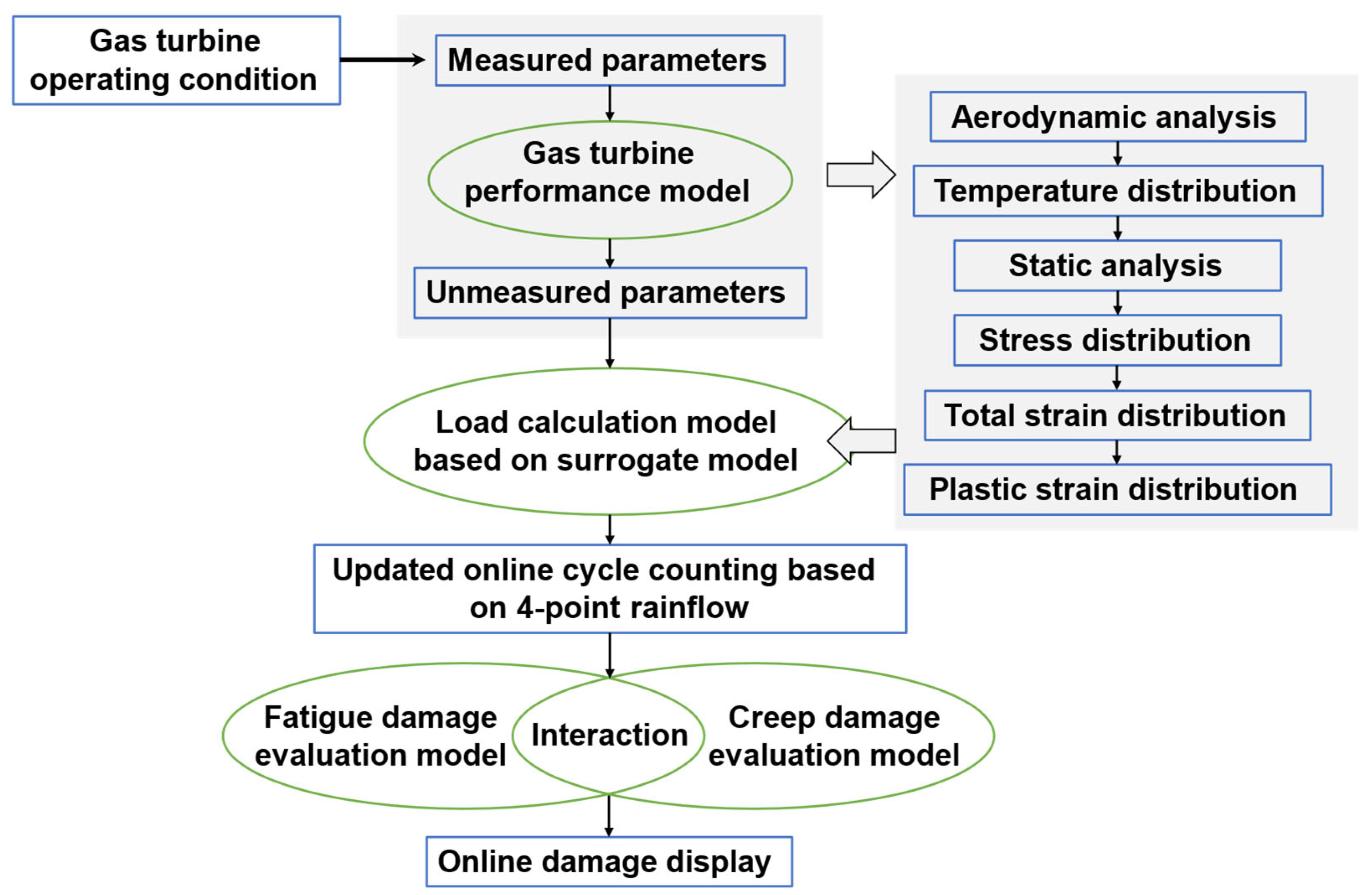
The gas turbine blade online damage evaluation model established in this study is a hybrid model, as shown in Figure 1. This model includes a gas turbine performance model based on thermodynamic simulation, a component load calculation model based on a surrogate model, an improved cycle counting method based on the four-point online rainflow counting method, and an improved damage mechanism evaluation model. The inputs of the online blade damage evaluation model established in this study include sensor measurements of environmental temperature/pressure, compressor inlet/outlet temperature/pressure, and other parameters. Parameters that cannot be directly measured using sensors are obtained with simulation using the gas turbine performance model, such as turbine inlet temperature/pressure and fuel flow rate. The simulation results from the performance model and the sensor measurements are used as inputs for the component load calculation model based on the surrogate model. Subsequently, the blade load information is processed using the improved cycle counting method and serves as input for the damage mechanism evaluation model. In this evaluation, the interactional damage of the blade is evaluated based on the results of the creep and fatigue analysis.
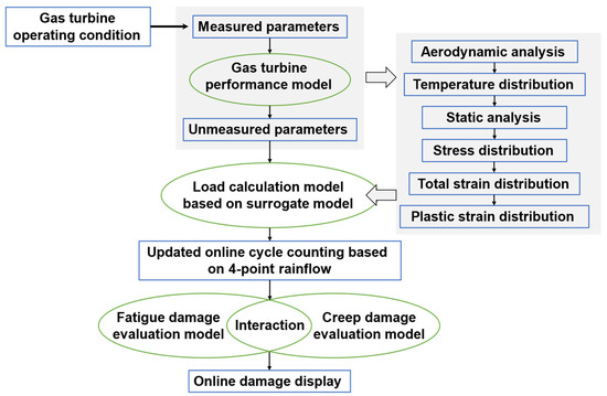
Figure 1.
A simplified flow diagram of the online damage evaluation model.
2.1. Gas Turbine Performance Model
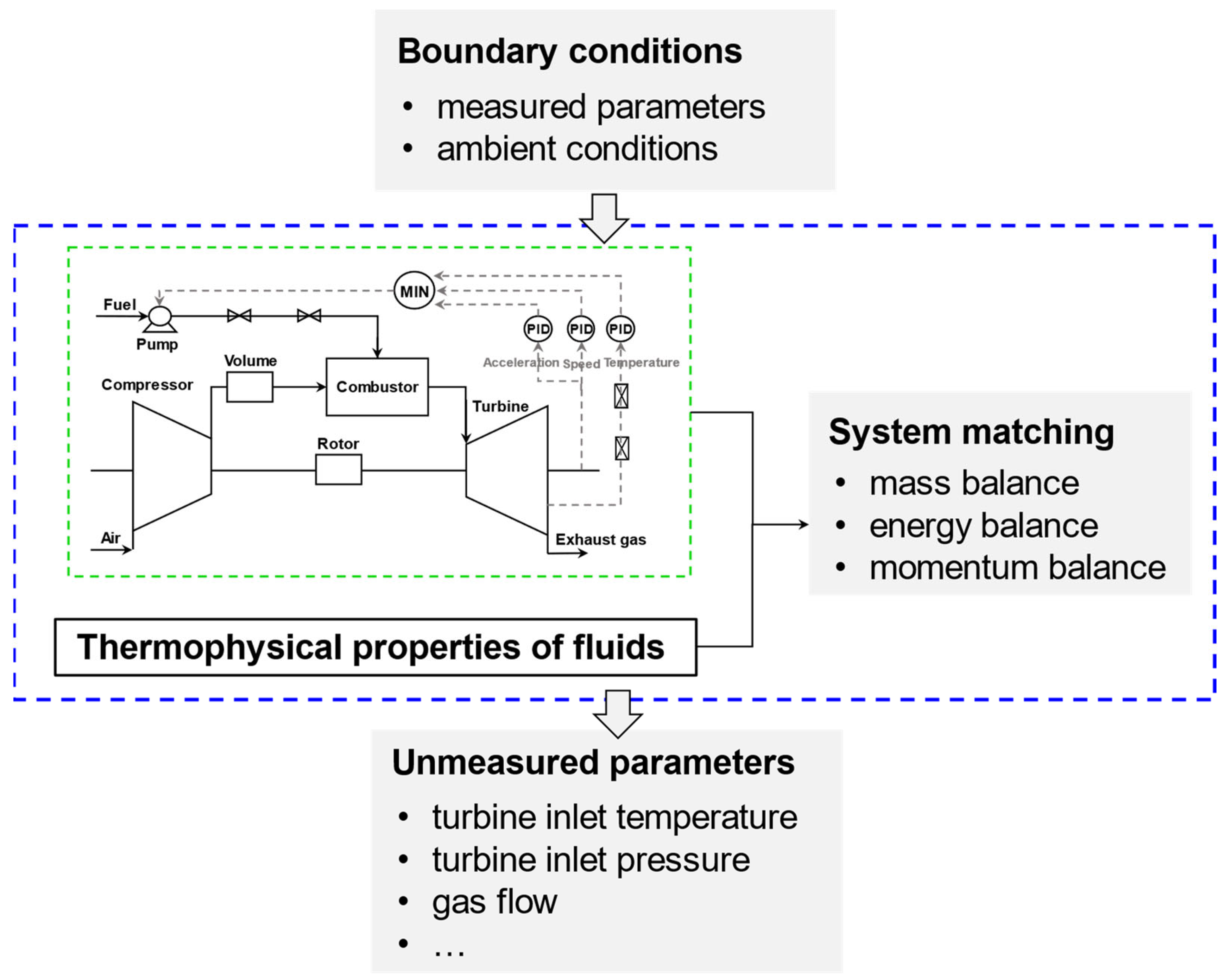
To calculate the blade load information, it is necessary to obtain parameters that cannot be measured directly using sensors, such as turbine inlet temperature/pressure and fuel flow rate. The aforementioned parameters can be derived with calculations using the gas turbine performance model and the measured parameters from sensors. Therefore, this study uses a modular modeling approach [29,30], where component models for the compressor, combustion chamber, turbine, rotor, and other parts are established. Based on the principles of mass conservation, energy conservation, and momentum conservation, the thermophysical properties of the fluid are matched with the system. A no-deficit control speed control logic is implemented to set the no-deficit regulation speed, and a gas turbine performance simulation model is developed. A flowchart illustrating the process is shown in Figure 2. The parameters deviating from the design point are obtained using referencing characteristic curves.
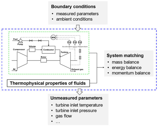
Figure 2.
A simplified scheme of the gas turbine performance model.
2.2. The Load Calculation Model Based on the Surrogate Model
The construction of a surrogate model for obtaining real-time blade load information in hazardous zones based on the operating condition of a gas turbine can be divided into two steps.
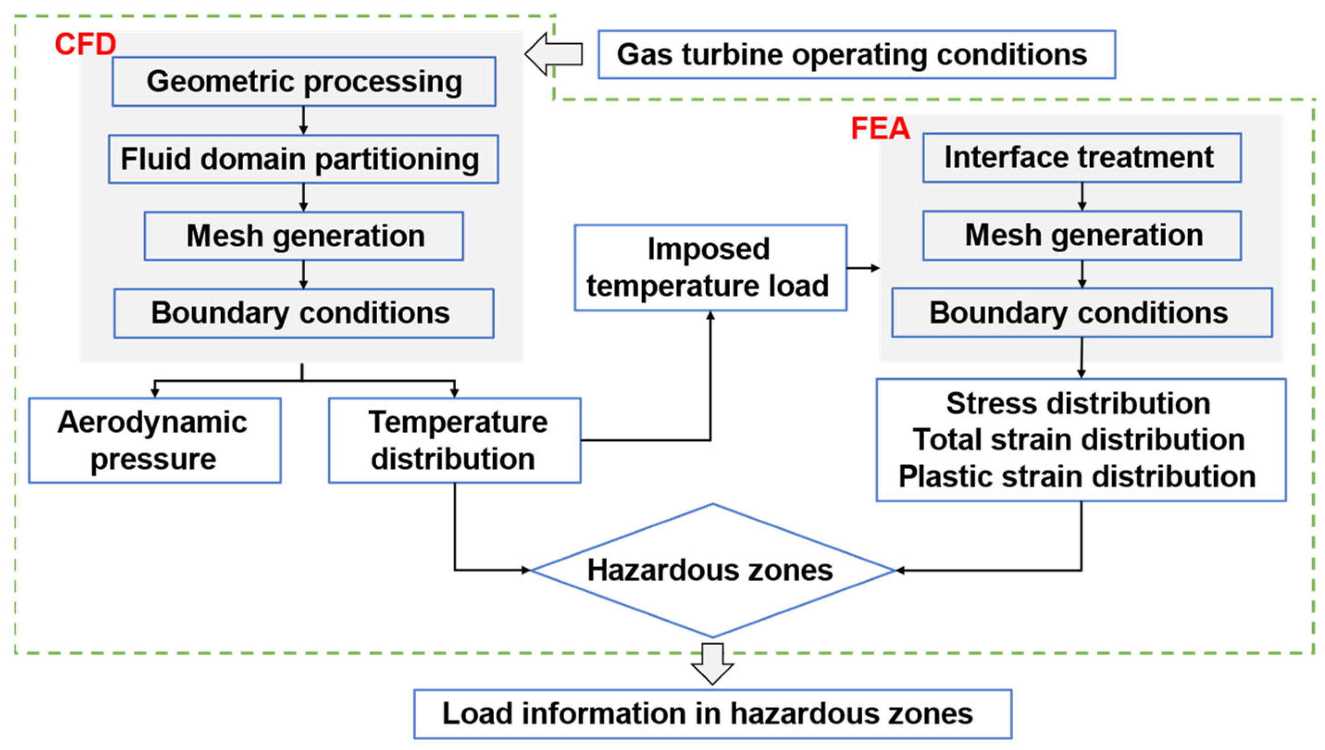
The first step is to obtain a dataset for training the surrogate model using simulation calculations. Among them, the temperature distribution of the blade is a prerequisite for stationary analysis. It is necessary to first obtain the temperature distribution of the blade under different operating conditions of the gas turbine using CFD. Then, based on the temperature distribution of the blade, the stress distribution of the blade under the current operating condition is calculated. Finally, the blade’s hazardous zones are determined by integrating the results of both calculations. For a detailed analysis process, please refer to Figure 3. It should be noted that in this study, FEA is conducted using an elastoplastic model.
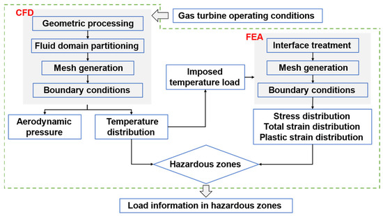
Figure 3.
Scheme of CFD and FEA.
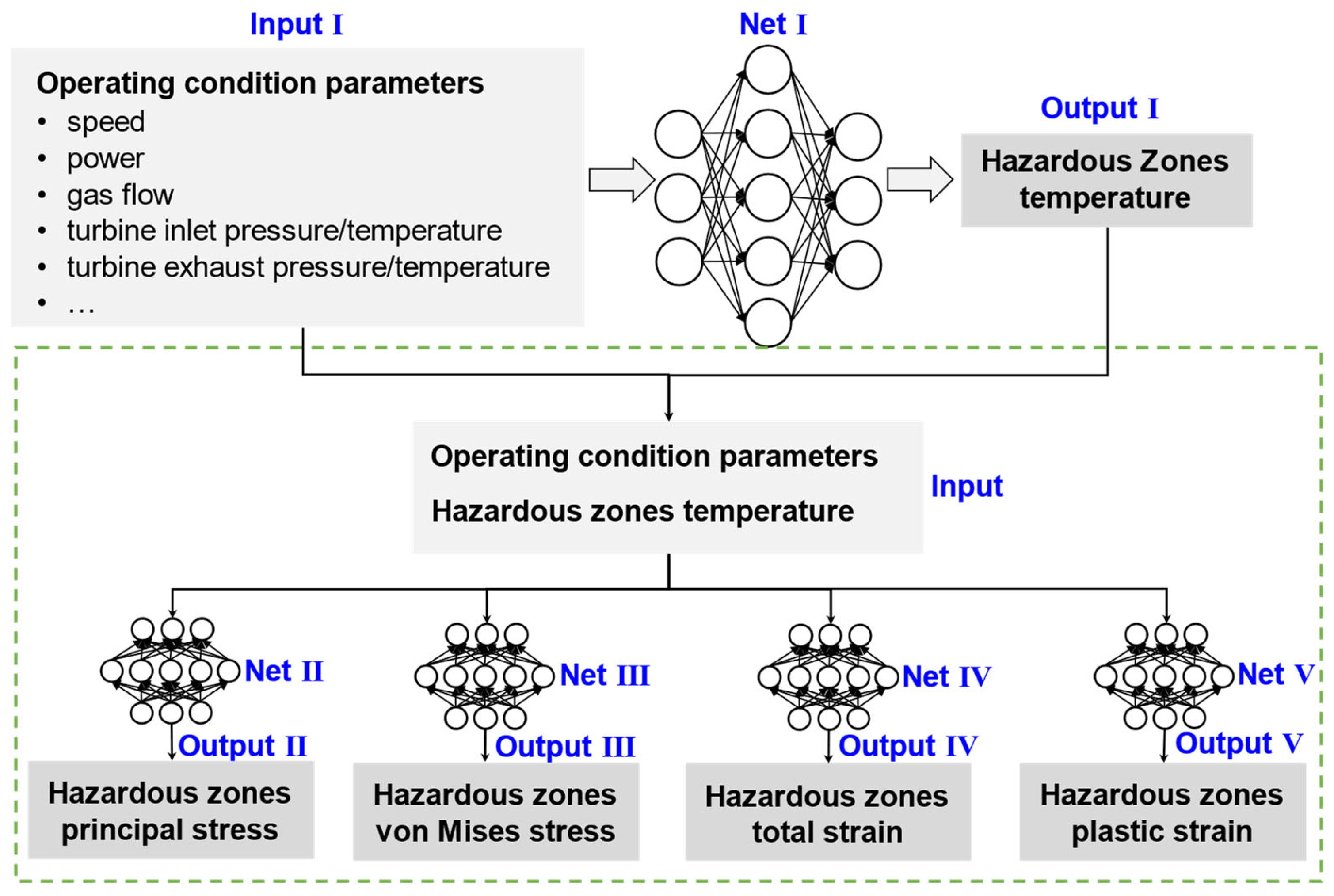
The second step is to train the surrogate model based on the results of CFD and elastoplastic FEA. The surrogate model is constructed based on an LSTM (long short-term memory) neural network. The input of the model is the operating state parameters of the gas turbine, and the output is the temperature information of the blade in the hazardous zones. Similarly, using the operating state parameters of the gas turbine and the results of the temperature calculation surrogate model as input, and the first principal stress, equivalent stress, total strain, and plastic strain in the hazardous zones of the blade as output, a surrogate model for stress calculation purposes is constructed. For a detailed analysis process, please refer to Figure 4.
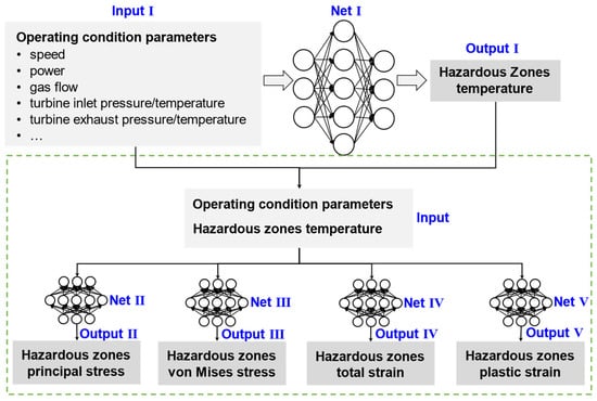
Figure 4.
Scheme of the surrogate model.
It should be noted that the von Mises stress obtained using FEA can only represent the magnitude of the stress and not its direction. Throughout the operating cycle, the blade experiences both tensile and compressive stresses, and failure to consider their respective directions can result in significant errors in estimating the stress range. In this study, the tensile and compressive states in the hazardous zone are determined based on the sign of the maximum principal stress, σ1. When σ1 > 0, the hazardous zone is subjected to tensile stress, and when σ1 < 0, the hazardous zone is subjected to compressive stress.
2.3. Updated Online Cycle Counting Based on the Four-Point Rainflow Counting Method
This study proposes an online cycle counting method that takes into account load fluctuations during the cyclic process, based on the four-point rainflow counting method [28]. The algorithm takes the real-time load information of the hazardous zones of the blade as input, which is calculated based on the surrogate model. The counting rules slightly differ for different counting objects, and this study introduces them in two parts, one by one.
2.3.1. Temperature Counting
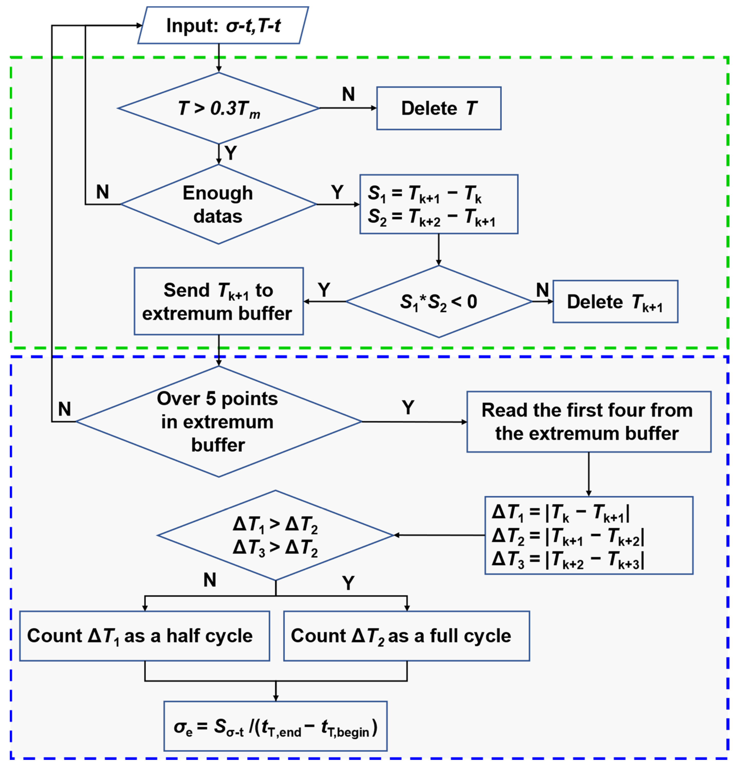
When evaluating creep damage, counting the incoming temperature information is crucial. The characteristic stress, which represents the cyclic stress information, is chosen based on the duration of the cycle. The detailed process is shown in Figure 5.
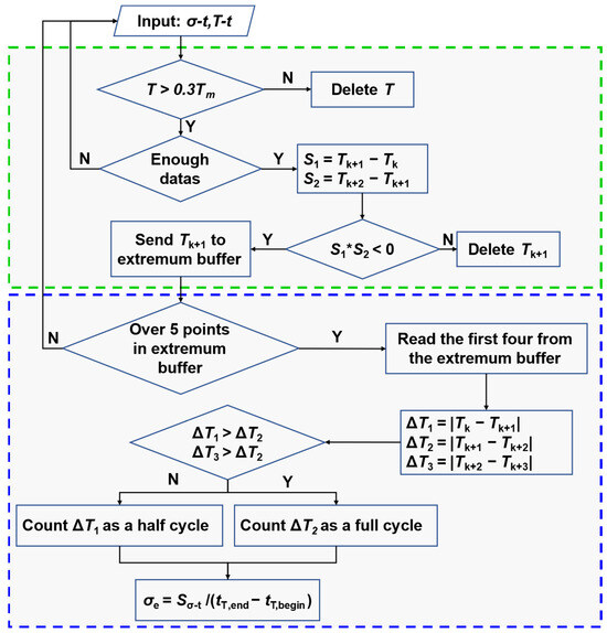
Figure 5.
Flowchart of the updated online cycle temperature counting.
The updated cycle counting method for temperature counting primarily consists of two parts: effective temperature extraction and extreme value identification, as well as full cycle/half cycle determination and cycle counting. As shown in Figure 5, this process begins with reading the input data, including the temperature value T and stress value σ corresponding to the latest time point t. The counting process begins when the read temperature value T exceeds 30% of the melting point temperature of the metal material. Once three data points are read, the extreme values can be identified. Assuming the stress values of three consecutive temperature readings are Tk, Tk+1, and Tk+2, if (Tk+1 − Tk)(Tk+2 − Tk+1) < 0, then Tk+1 is considered as an extreme value point, and it should be stored in the extremum buffer. On the other hand, if (Tk+1 − Tk)(Tk+2 − Tk+1) > 0, then Tk+1 is not an extreme value point and should be excluded from further consideration. At the same time, the rainflow counting method based on four points requires at least four extreme values before determining the cycle type. Let us assume that the four consecutive extreme values retrieved from the extremum buffer are T1, T2, T3, and T4. We can calculate the differences as follows: ΔT1 = |T1 − T2|, ΔT2 = |T2 − T3|, and ΔT3 = |T3 − T4|. If ΔT2 < ΔT1 and ΔT2 < ΔT3, then it is considered as a full cycle. Otherwise, it is considered as a half cycle and ΔT1 represents the half cycle. This study refers to the references by GopiReddy [31,32] on the rainflow counting method for online evaluation of creep damage, where the relationship between load information and load duration in the case of full cycles is proposed. This study introduces the concepts of cycle start time tT,begin, cycle end time tT,end, and cycle duration tT,hold when considering full cycles. The calculation formulas are as follows:
where t1, t2, t3, and t4 represents the time corresponding to T1, T2, T3, and T4 respectively.
tT,begin = t2
tT,hold = tT,end − tT,begin
For half cycles, the calculation formula for the time information is as follows:
tT,begin = t1
tT,end = t2
tT,hold = tT,end − tT,begin
Research has shown that for materials where the stress–strain curve is temperature-dependent, the time required for the complete formation of local magnetic hysteresis loops is crucial in the calculation of average temperature. Therefore, this study uses the concept of equivalent mean temperature proposed by GopiReddy [31], which refers to the time-weighted average temperature over the entire cycle. In the case of full cycles, the calculation formula is as follows:
In the case of half cycles, the equivalent mean temperature is directly taken as the mean temperature of the two. The calculation formula is as follows:
where represents the equivalent mean temperature.
The characteristic stress represents a parameter that represents the cycle stress–time history. In order to enhance the accuracy of creep damage evaluation, this study takes the time-weighted stress over the entire duration of the identified cycle as the characteristic stress of that cycle. Mathematically, it can be expressed as follows:
where represents the characteristic stress of the identified cycle and represents the area of the polygon in the σ−t diagram.
2.3.2. Stress Counting
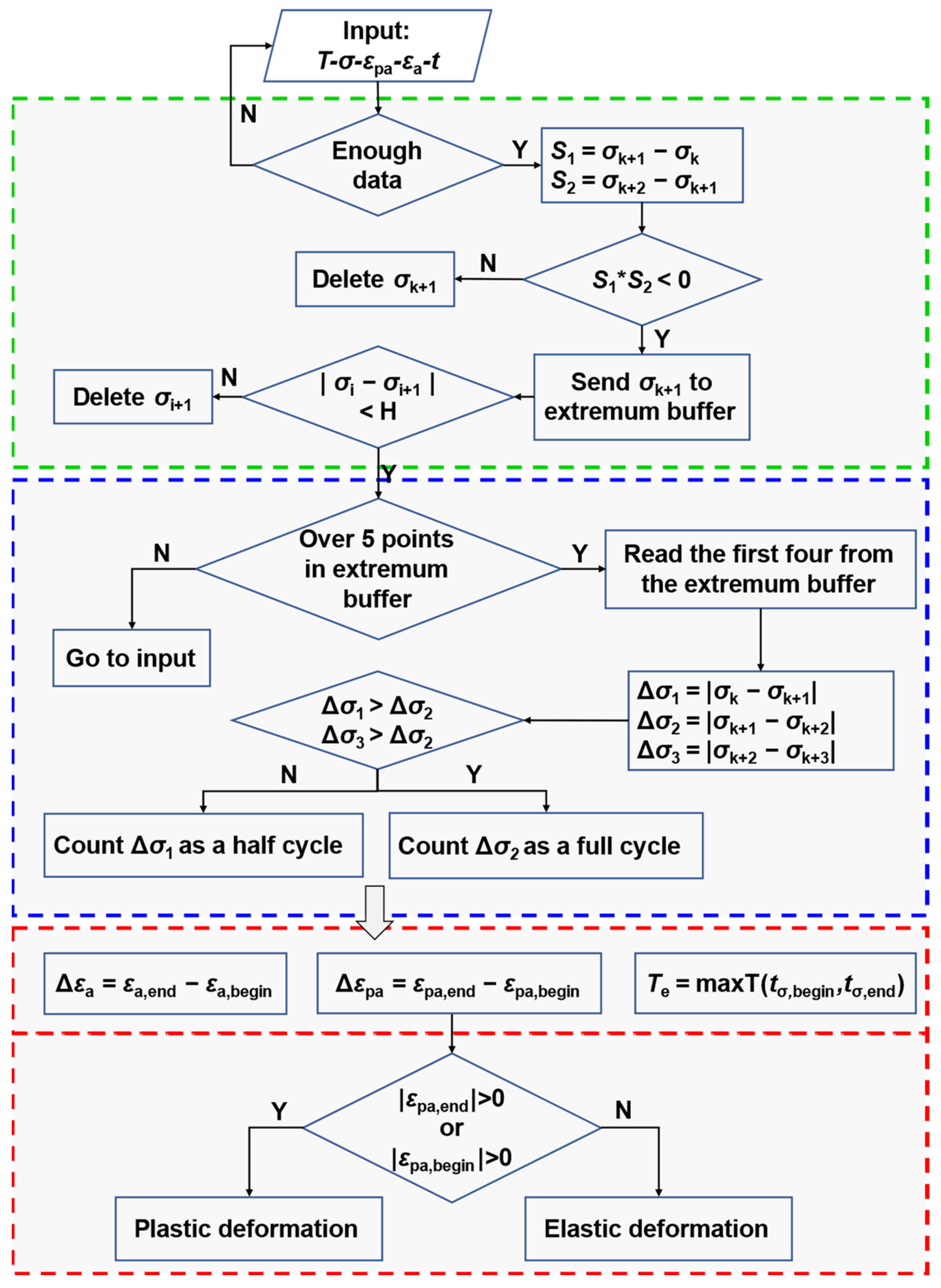
When evaluating fatigue damage, the incoming stress information is counted, and a characteristic temperature representing the cycle temperature information is selected based on the cycle duration. The total strain and cyclic plastic strain are also determined based on the duration of the cyclic loading. The detailed process is shown in Figure 6.
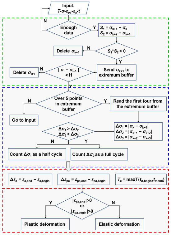
Figure 6.
Flowchart of the updated online cycle stress counting.
The updated stress counting method for cycle counting mainly includes three parts: peak identification and removal of invalid amplitudes, determination of full cycle/half cycle and cycle counting, matching characteristic temperature, and deformation mechanism determination. As shown in Figure 6, the process starts with reading the input data, which includes the temperature value T, stress value σ, total strain value εa, and plastic strain value εpa corresponding to the latest time point t. The peak identification process is similar to temperature counting in nature. The purpose of removing invalid amplitudes is to eliminate insignificant fluctuations in damage accumulation. The determination of invalid amplitudes requires a threshold value H to be defined. This threshold value H is influenced by multiple variables such as gas turbine structure, operating speed, output power, etc. The value of H varies under different conditions. It should be noted that the determination of the threshold value H does not affect the method proposed in this study.
The determination of cycle types and temperature counting also follows a similar approach. When the full cycle condition is satisfied, the maximum stress of the cycle is given by σmax = max(σ2, σ3), the stress amplitude is calculated as σa = (|σ2 − σ3|)/2, the mean stress is determined as σm = (σ2 + σ3)/2, and the cycle count is incremented by 1. The points σ2 and σ3 are removed, while σ1 and σ4 are retained. The process then continues by reading a new incoming data point and restarting the identification process. The relationship between the loaded information and the loaded time during the reference temperature counting is considered, leading to the introduction of the concepts of cycle start time tσ,begin, cycle end time tσ,end, and cycle duration tσ,hold specifically for full cycles. These concepts are illustrated in Figure 7, and their calculation expressions are as follows:
where t1, t2, t3, and t4 represents the time corresponding to σ1, σ2, σ3, and σ4 respectively.
tσ,begin = t2
tσ,hold = tσ,end − tσ,begin
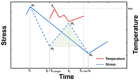
Figure 7.
Schematic diagram of the stress–time relationship during a full cycle.
When the half cycle condition is satisfied, the maximum stress of the cycle is given by σmax = max(σ1, σ2), the stress amplitude is calculated as σa = (|σ1 − σ2|)/2, the mean stress is determined as σm = (σ1 + σ2)/2, and the cycle count is incremented by 0.5. The point σ1 is removed, while σ2, σ3, and σ4 are retained. The process then continues by reading a new incoming data point and restarting the identification process. The calculation formula for the time information of the cycle in this case is as follows:
tσ,begin = t1
tσ,end = t2
tσ,hold = tσ,end − tσ,begin
The characteristic temperature refers to the parameter that best represents the temperature history of the identified cycle. It is important to note that temperature directly affects various properties of the material, and different materials may have different criteria for selecting characteristic temperatures. In this study, the maximum temperature experienced throughout the entire process from the start to the end of the identified cycle is considered as the characteristic temperature of that cycle. Therefore, the characteristic temperature of the cycle is determined as follows:
where Te represents the characteristic temperature of the identified cycle.
The plastic strain generated during plastic deformation of a material is the primary factor contributing to fatigue damage. When a material undergoes elastic deformation, the plastic strain is zero. This study incorporates the time information of the identified cycle and provides the following formula for calculating the cyclic plastic strain in relation to the total strain:
where εpa,end represents the plastic strain at the end of the cycle, εpa,begin represents the plastic strain at the beginning of the cycle, Δεpa denotes the range of plastic strain identified in the cycle, εa,end represents the total strain at the end of the cycle, εa,begin represents the total strain at the beginning of the cycle, and Δεa denotes the range of total strain identified in the cycle.
Δεpa = εpa,end − εpa,begin
Δεa = εa,end − εa,begin
2.4. Creep–Fatigue Damage Evaluation Model
This study conducts real-time damage evaluation of a blade based on the load information obtained using the online cycle counting method. During the damage evaluation, the damage caused by various damage mechanisms is considered independently to decouple the effects of each mechanism. In the evaluation of creep damage, the influence of temperature and stress fluctuations is taken into account. In the evaluation of fatigue damage, the influence of temperature fluctuations is considered.
2.4.1. Creep Damage Evaluation Model
Creep damage evaluation in engineering typically considers only the damage caused by the steady-state operation of gas turbines while ignoring the creep damage resulting from load fluctuations during steady-state operation and non-steady-state operation. As a result, this approach can lead to significant errors in the evaluation results and goes against the original intention of maintenance based on the operational status of gas turbines.
The Larson–Miller parameter method [33] is widely applied for evaluating creep damage, and it is the most commonly used approach. For the hazardous region of the blade, the expression is as follows:
where tr is stress rupture time or time to failure, T is the blade material temperature, is the stress at the corresponding zone, C is the material constant, and L is the Larson–Miller parameter (LMP).
Finally, the ratio of the cycle tT,hold to tr is used to quantify creep damage. The total creep damage is calculated by linearly summing up the creep damage for each cycle based on the Miner linear damage rule [34]. The representation is as follows:
where Dc represents the total creep damage.
2.4.2. Fatigue Damage Evaluation Model
As mentioned above, effective full-cycle and half-cycle were identified during stress counting, and the characteristic temperature of each identified cycle was determined, as well as the damage mechanism caused by each cycle on the blade. This section will match the appropriate damage evaluation models based on the blade’s damage mechanism.
When the blade does not undergo plastic deformation, this study uses the SWT model, which considers ∆εa, σmax, and temperature fluctuations for damage evaluation. The representation of the SWT model [18] is as follows:
where represents the fatigue strength coefficient, b represents the fatigue strength exponent, represents the fatigue ductility coefficient, c represents the fatigue ductility exponent, and represents the maximum number of cycles under the current load condition.
In (21), , E, b, , and c are all functions of temperature. In this study, considering the influence of temperature fluctuations on fatigue damage, the aforementioned parameters are selected based on the characteristic temperature identified for each cycle.
When plastic deformation occurs in the component, this study uses a new model [35] that takes into account the influence of ∆εpa, ∆εa, and σmax on cyclic damage. Furthermore, the model introduces a function f(T) to describe the effect of temperature variation on fatigue life. The form of the temperature correction term in the new model and the validation of its accuracy were previously completed in prior work. It is represented as follows:
where A represents the correction term considering the influence of temperature and n1~n3 are undetermined constants.
Finally, for full cycles, the reciprocal of the maximum number of cycles under the current load condition is used as the fatigue damage for that cycle. However, for half cycles, only half of the reciprocal of the maximum number of cycles under the current load condition is used as the fatigue damage for that cycle. According to the Miner linear damage rule, the total fatigue damage is calculated by linearly summing up the fatigue damage for each cycle. It is represented as follows:
where Df represents the total fatigue damage, n represents the number of cycles for the i-th cycle, and C(i) is a constant used to determine the type of the i-th cycle, which takes the value of 1 for a full cycle and 0.5 for a half cycle.
2.4.3. Creep–Fatigue Interaction Damage Evaluation Model
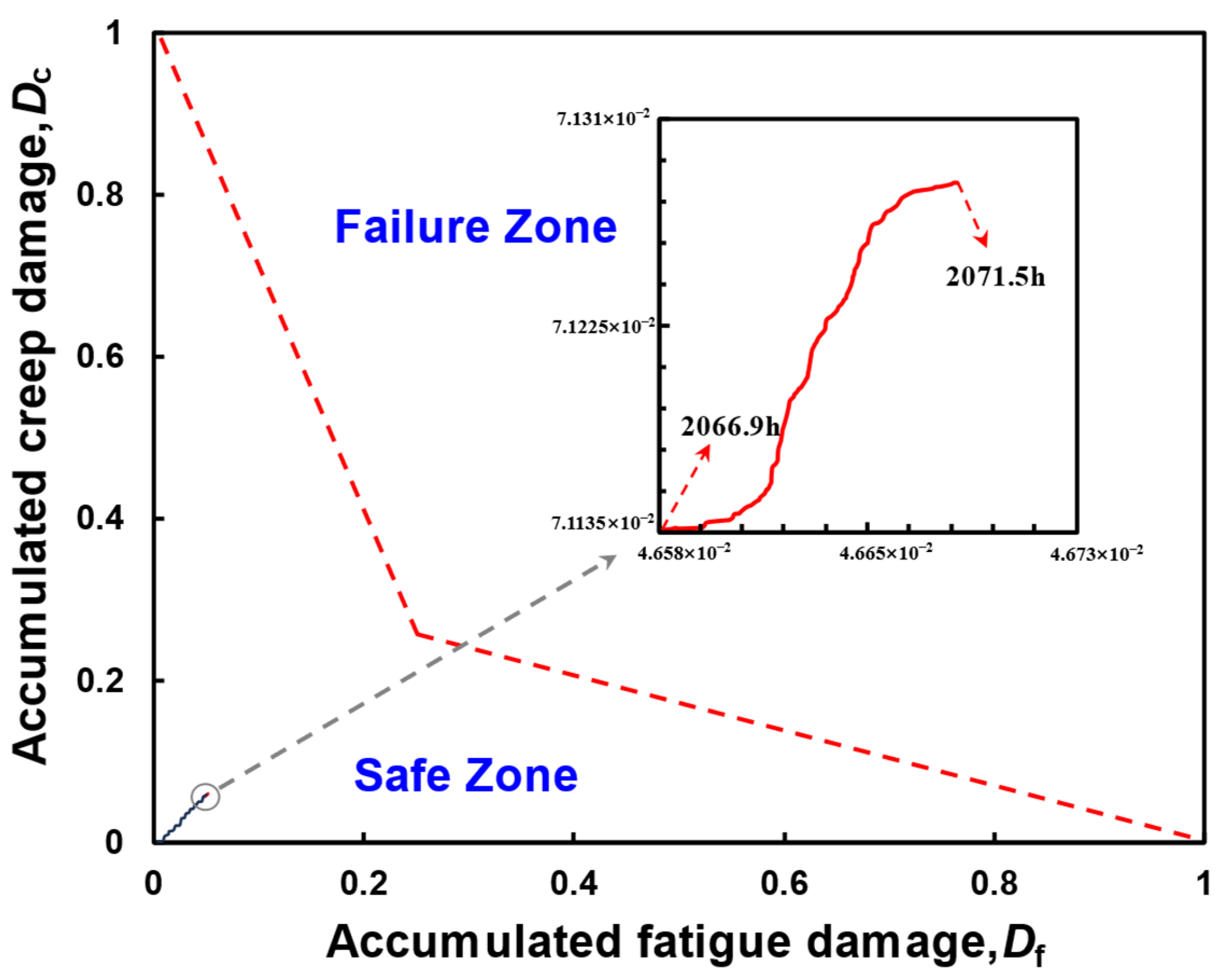
There exists a complex interaction between fatigue and creep; thus, fatigue damage and creep damage at a given point cannot be considered separately. To address this, numerous damage evaluation models have been proposed by scholars both domestically and internationally, such as the strain energy density depletion model [36] and the modified ductility exhaustion model [37]. One of the evaluation models based on the fatigue–creep damage assessment chart [38] can dynamically display the evolution of fatigue–creep damage state, making it highly suitable for online assessment of the health condition of a blade, as shown in Figure 8. It can be mainly divided into three parts: the axis representing accumulated fatigue/creep damage, the life criteria line determined with experimental data, and the safe zone and failure zone distinguished by design criteria.
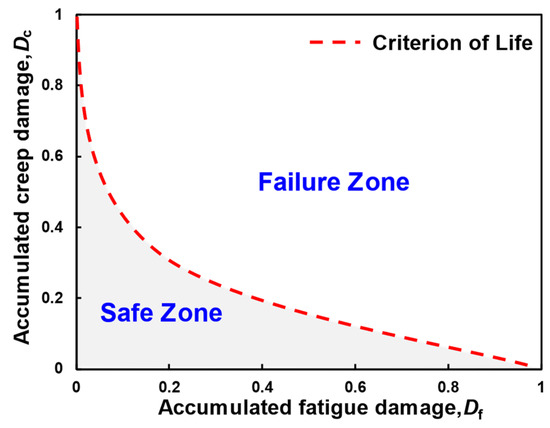
Figure 8.
Creep–fatigue damage evaluation chart.
3. Experiment and Discussion
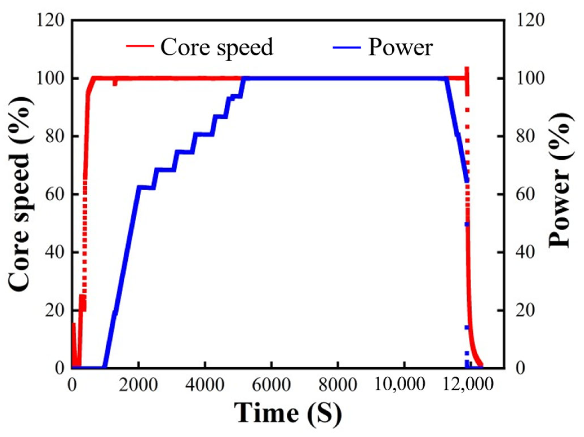
This study validates the feasibility of the established online blade damage evaluation model based on operational data of a micro gas turbine in the “cold start-steady state-shutdown” operating mode. The design parameters of the micro gas turbine are presented in Table 1, while the operational data for the “cold start-steady state-shutdown” mode are illustrated in Figure 9.

Table 1.
Micro gas turbine parameters.

Figure 9.
The operational data of the micro gas turbine.
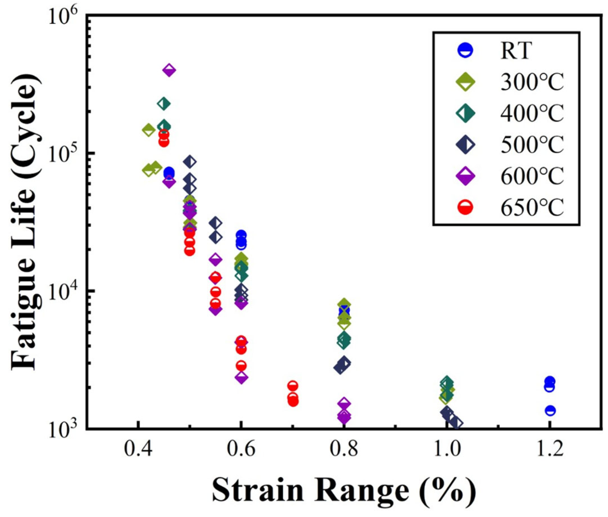
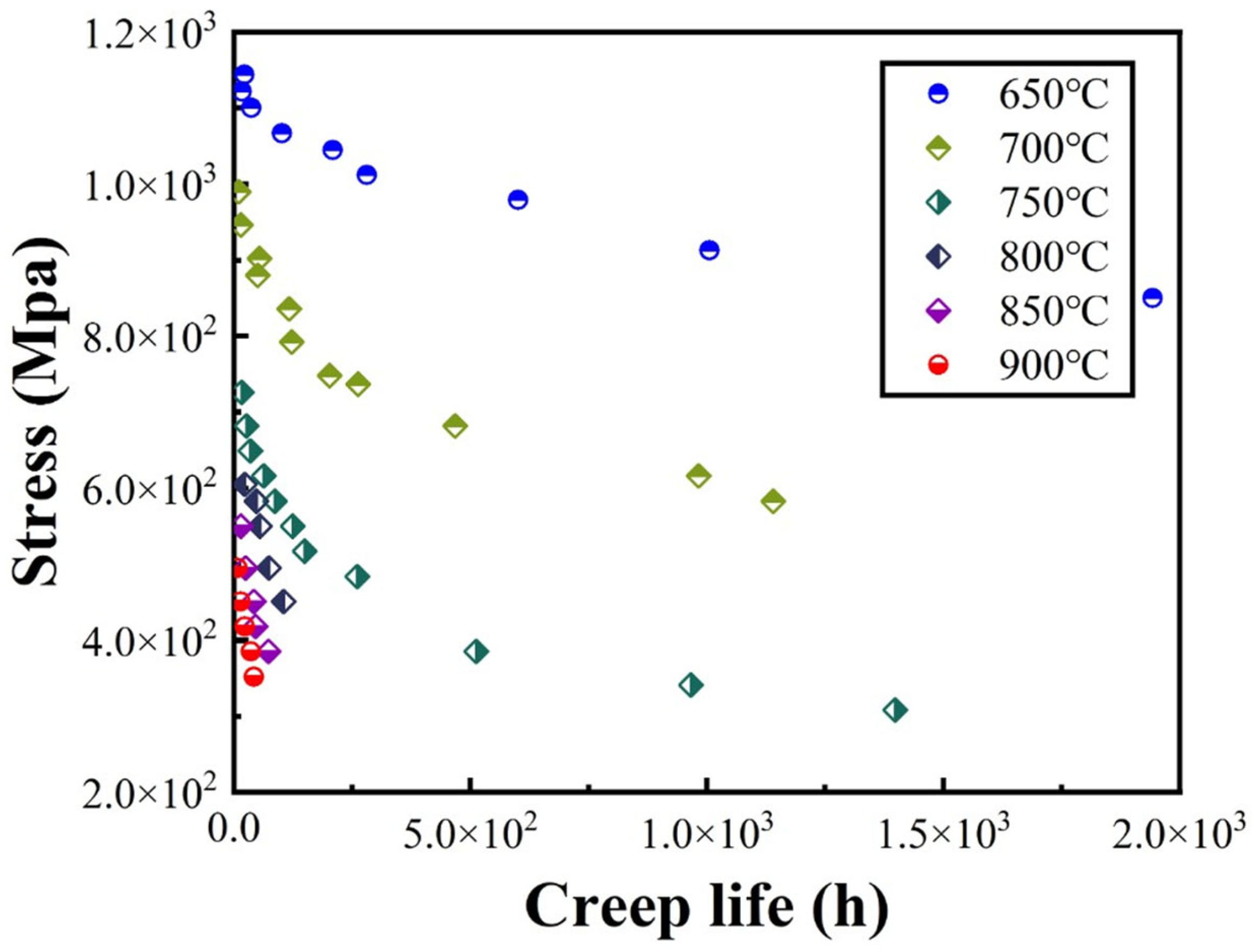
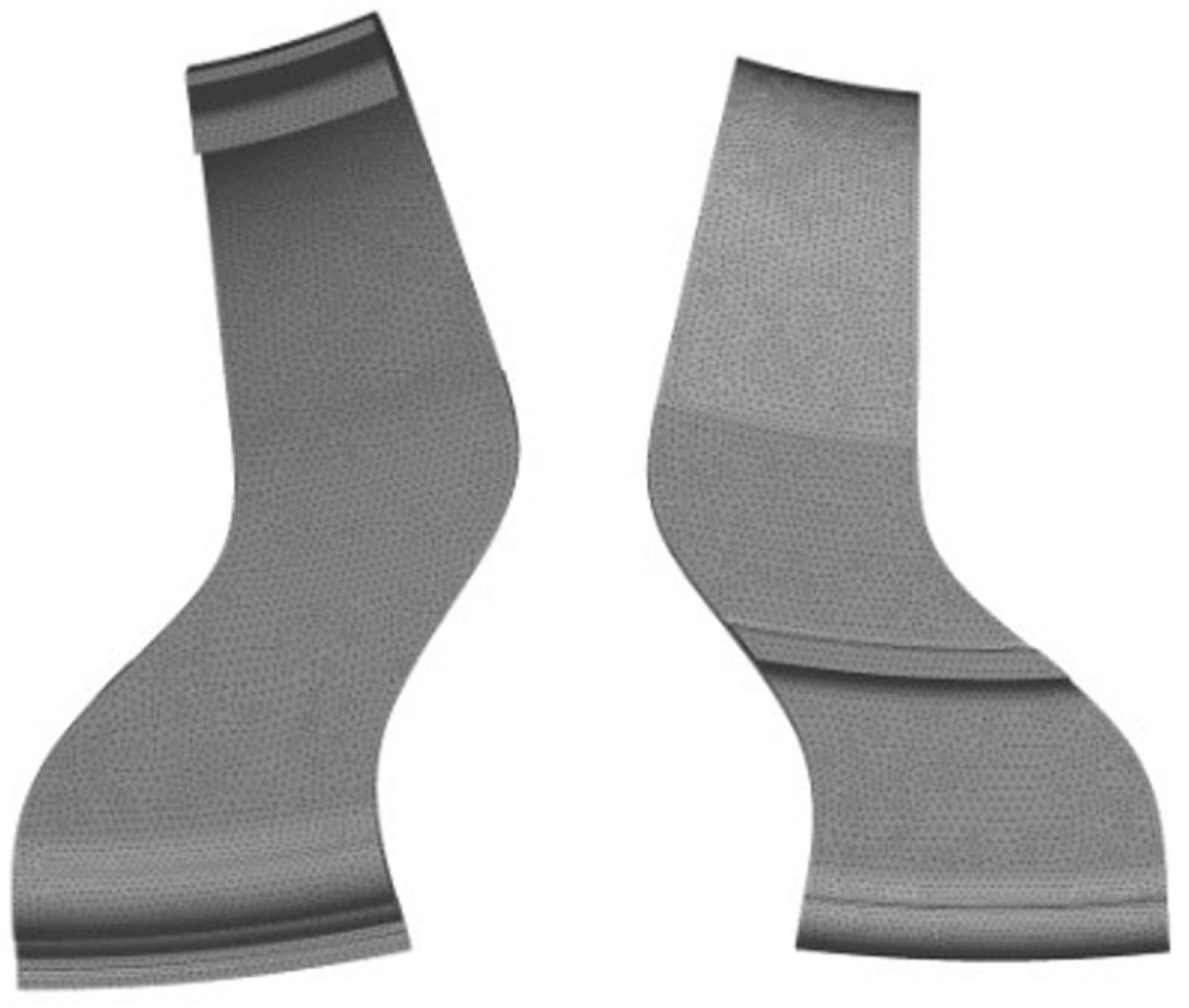
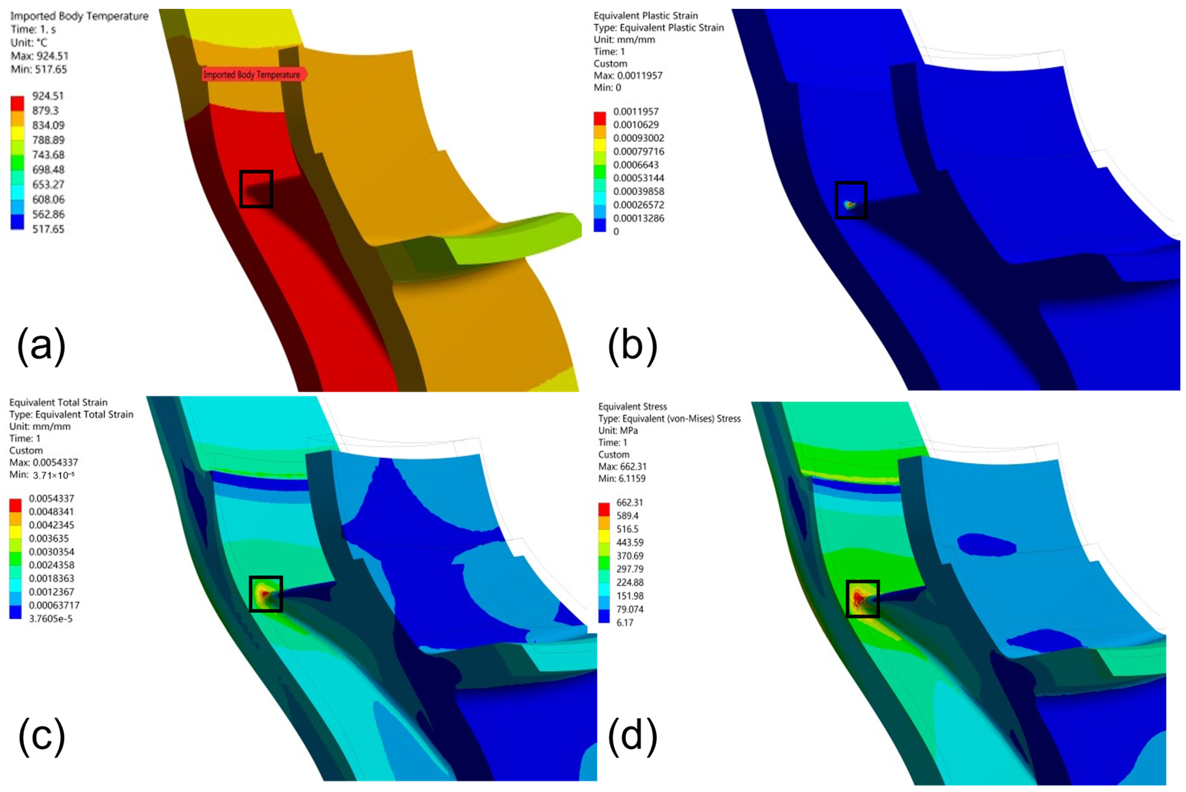
In this study, the turbine stationary blade of the selected gas turbine is chosen as the research object for simulation and calculation. The turbine stationary blade is made of a certain nickel-based high-temperature alloy, and its fatigue and creep properties are shown in Figure 10 and Figure 11. Referring to the operational data in Figure 9, a total of 245 typical transient points, where there are abrupt changes in speed and power, are selected. The open-source finite element software CalculiX (http://www.calculix.de, accessed on 28 September 2023) is used for temperature field calculation and stationary analysis. The temperature field calculation is performed based on the 2D computational method, while the stationary analysis uses an elastic–plastic finite element model. To mitigate the computational time cost, only 1/29 of the entire turbine stationary blade is selected for analysis. The mesh structure of this selected portion is illustrated in Figure 12. Based on the calculation results of the 245 transient points, it is determined that the leading edge of the turbine stationary blade is the critical region. The distribution of the load at steady state is depicted in Figure 13a–d.
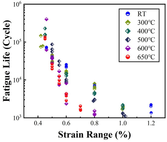
Figure 10.
Schematic diagram of the fatigue properties of the turbine stationary blade material.

Figure 11.
Schematic diagram of the creep properties of the turbine stationary blade material.

Figure 12.
The mesh structure of the turbine stationary blade.
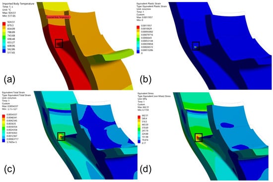
Figure 13.
The (a) temperature, (b) equivalent plastic strain, (c) equivalent total strain, and (d) equivalent stress distribution of a certain transient point at steady state.
This study determines the tensile and compressive states of the hazardous zone based on the positive and negative values of the maximum principal stress. The distribution of maximum principal stress for a certain transient point during the start-up, steady state, and shutdown processes is illustrated in Figure 14. It should be noted that in this study, the gas turbine is considered to be in a shutdown state when it no longer outputs power. However, at this stage, the temperature of various components remains high, which may result in residual stress. The damage caused by residual stress is not taken into consideration in this study. Based on the above analysis and considering Figure 14, it can be assumed that the hazardous zone of the gas turbine stationary blade is subjected to compressive stress throughout the “cold start-steady state-shutdown” process.

Figure 14.
The maximum principal stress distribution of a certain transient point at (a) cold start, (b) steady state, and (c) shutdown.
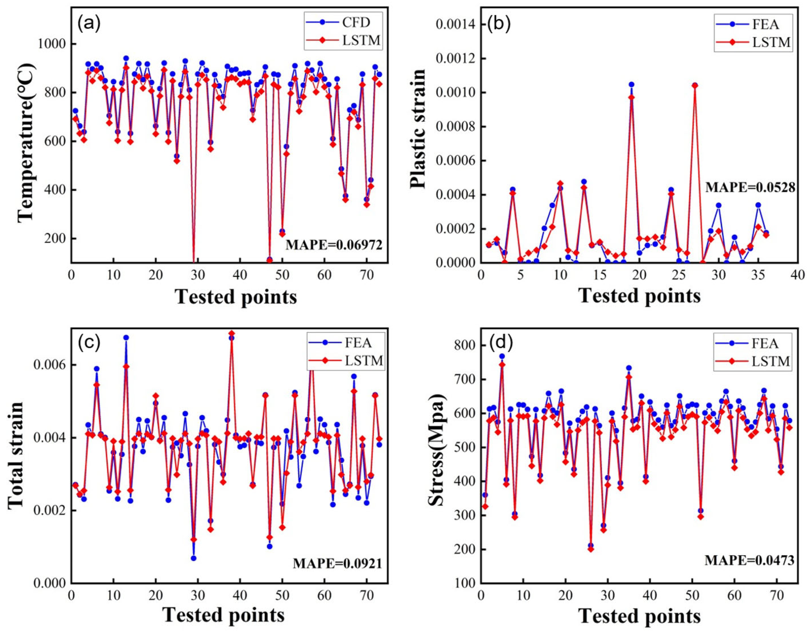
During the entire operational process, the load on the turbine stationary blade undergoes continuous variations, while the selected transient points can only reflect the load information at the current moment. To obtain the load information of the turbine stationary blade throughout the entire operational process, this study uses the aforementioned load calculation model based on the surrogate model. It is worth noting that while the turbine stationary blade is a non-rotating component, the motion of the rotor driving the moving blade increases fluid turbulence within the turbine, enhances heat exchange between the fluid and various components, and consequently influences the temperature distribution of the turbine stationary blade [39]. The model takes the selected typical transient points’ power, rotational speed, fuel flow rate, and temperature/pressure at the inlet/outlet of the turbine as inputs, and outputs the simulated load information of the identified hazardous zone. The surrogate model is trained accordingly. The training set and test set are divided in a ratio of 7:3, and the model’s test results are shown in Figure 15a–d. The results show that the MAPEs of the surrogate model in calculating temperature, total strain, plastic strain, and stress are all less than 10%, indicating that the accuracy of the surrogate model is within an acceptable range. Finally, using the surrogate model, the loading condition of the turbine stationary blade in the hazardous zone throughout the entire “cold start-steady state-shutdown” process is obtained by traversing, as shown in Figure 16.
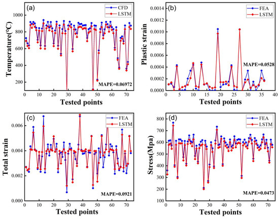
Figure 15.
Comparison between simulation results and surrogate model results: (a) temperature, (b) equivalent plastic strain, (c) equivalent total strain, and (d) equivalent stress.
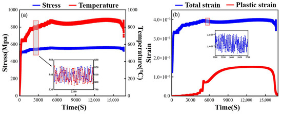
Figure 16.
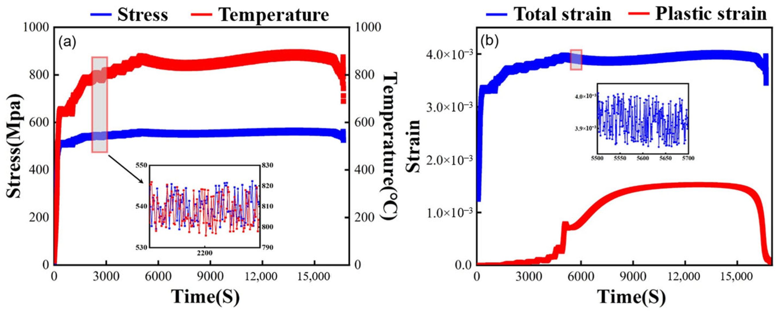
The load information of the turbine stationary blade in the hazardous zone throughout the entire “cold start-steady state-shutdown” process: (a) stress and temperature and (b) total strain and plastic strain.
Based on the overall structural arrangement, component material selection, and operating conditions of this micro gas turbine, the threshold value H for stress counting is set at 10 MPa, and the threshold value Tm for temperature counting is set at 450 °C. The data in Figure 16 are sampled every second. The updated cycle counting method based on the four-point online rainflow counting method is used in this study to perform cycle counting on the inflow load information. By applying the obtained real-time temperature spectrum and stress spectrum to the damage evaluation model, the fatigue damage Df of the micro turbine stationary blade during the process is calculated as 1.3065 × 10⁻⁴, and the creep damage Dc is calculated as 1.6303 × 10⁻⁴. In this study, a bilinear criterion is temporarily established to evaluate the interaction between the two types of damage, as shown in Figure 17. It should be noted that the provided lifetime criterion in this study is hypothetical. To determine an accurate lifetime criterion, relevant experiments need to be conducted.
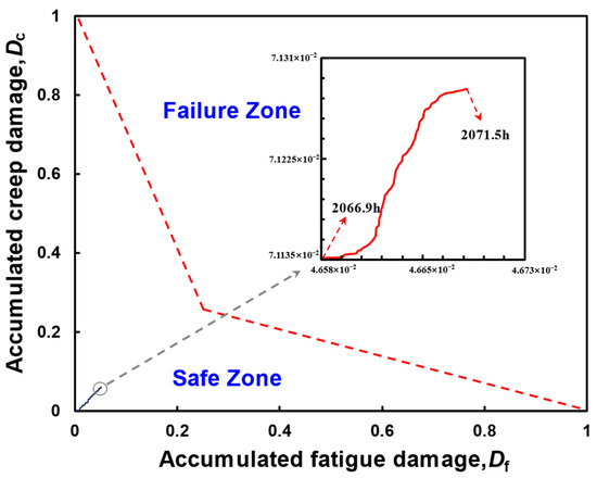
Figure 17.
Fatigue–creep damage assessment chart.
The OEM recommends that the major overhaul cycle for this micro gas turbine under base load conditions is 32,000 h or 700 start–stop cycles. The calculation formula for the EOH of this micro gas turbine is shown below:
where Cstart is the start-up weighting factor, Nstart is the start-up count, Cload change is the load change weighting factor, Nload change is the load change count, Ctrip is the trip weighting factor, Ntrip is the trip count, Cstress is the stress weighting factor, Cfuel is the fuel weighting factor, Time is the actual operating hours.
EOH = Cstart [Nstart + Cload changeNload change + CtripNtrip] + CstressCfuelTime
Based on (24), it can be determined that, after undergoing the aforementioned process, the damage DOEM to the micro gas turbine stationary blade is calculated as 4.475 × 10⁻⁴. The OEM’s recommended value is slightly higher than the calculated results of this model, possibly because the OEM considers erosion, abrasion, oxidation corrosion, or other damage mechanisms when calculating the damage to the blade.
4. Conclusions
This study established a hybrid model for gas turbine blade online damage evaluation based on operating conditions. This model includes a gas turbine performance model based on thermodynamic simulation, a component load calculation model based on a surrogate model, an improved cycle counting method based on the four-point online rainflow counting method, and an improved damage mechanism evaluation model. Based on the experimental data for the “cold start-steady state-shutdown” for a micro gas turbine, an online evaluation of the damage to the turbine stationary blade was conducted. The evaluation results of the model compared with the EOH suggested by the OEM showed a relative error of 34.37%, which preliminarily verified the practicality and feasibility of the model. This model can be applied to condition-based maintenance of gas turbine blades and other components. The same modeling approach can also be used in other fields such as online assessment of power semiconductor damage.
The novelty and originality of this study can be primarily categorized into two main parts:
- When obtaining blade load information based on gas turbine operating parameters, the new model utilizes a surrogate model instead of the traditional physics-based model. This improves the accuracy of blade load calculations and ensures real-time performance. However, the variable operating conditions, uncertain start/stop modes, and component degradation in gas turbines can all affect the blade load distribution. Incorporating these factors to build more complex surrogate models will be performed in our subsequent work.
- Regarding the online cycle counting method, the new model enhanced the conventional four-point online rainflow counting method to accommodate the counting of results from elastic–plastic analyses. Moreover, the inclusion of time information during cycle counting allows for the precise recording of load fluctuations, thereby providing accurate input conditions for a subsequent damage assessment. In addition, the online cycle counting method and damage evaluation model complement each other. Designing corresponding characteristic tests for different materials and finding the relationship between load conditions and their damage evolution can also improve the accuracy of the entire model.
Author Contributions
H.Z.: wrote this paper, performed research, analyzed the data; X.Z.: funding acquisition, designed research, revised this paper; J.C.: processed data and guided the simulation method; Y.Z.: analyzed data; M.L.: analyzed data; W.H.: supervision. All authors have read and agreed to the published version of this manuscript.
Funding
This research received no external funding. And the APC was funded by Shanghai Advanced Research Institute, Chinese Academy of Sciences.
Data Availability Statement
Data are contained within the article.
Conflicts of Interest
The authors declare no conflict of interest.
Nomenclature
| OEM | original equipment manufacturer |
| EOH | equivalent operating hours |
| LSTM | long short-term memory |
| CFD | computational fluid dynamics |
| FEA | finite element analysis |
| T | temperature |
| Tm | melting point temperature |
| equivalent mean temperature | |
| the area of the polygon in the σ−t diagram | |
| tr | stress rupture time |
| Larson–Miller parameter | |
| Te | characteristic temperature |
| t | time |
| H | threshold for invalid cycle determination |
| elastic modulus | |
| fatigue cycle count | |
| fatigue damage | |
| Dc | creep damage |
| damage recommended by the OEM | |
| Greek letters | |
| characteristic stress of the identified cycle | |
| maximum stress | |
| minimum stress | |
| stress amplitude | |
| mean stress | |
| εpa | plastic strain |
| εa | total strain |
| Δ | range |
| Subscripts | |
| T | temperature counting |
| stress counting | |
| begin | cycle start time |
| end | cycle end time |
| hold | cycle duration |
References
- You, Y.; Xu, J.; Yan, Q.; Zhang, W.; Guo, D.; Huang, T. Combined fatigue life prediction and experiment verification for turbine blade. J. Aerosp. Power 2022, 37, 946–953. [Google Scholar] [CrossRef]
- Liu, H.; Sun, J.; Lei, S.; Ning, S. In-service aircraft engines turbine blades life prediction based on multi-modal operation and maintenance data. Propuls. Power Res. 2021, 10, 360–373. [Google Scholar] [CrossRef]
- Sakib, N.; Wuest, T. Challenges and Opportunities of Condition-based Predictive Maintenance: A Review. Procedia CIRP 2018, 78, 267–272. [Google Scholar] [CrossRef]
- Prajapati, A.; Bechtel, J.; Ganesan, S. Condition based maintenance: A survey. J. Qual. Maint. Eng. 2012, 18, 384–400. [Google Scholar] [CrossRef]
- Kumar, S.; Mukherjee, D.; Guchhait, P.K.; Banerjee, R.; Srivastava, A.K.; Vishwakarma, D.N.; Saket, R.K. A Comprehensive Review of Condition Based Prognostic Maintenance (CBPM) for Induction Motor. IEEE Access 2019, 7, 90690–90704. [Google Scholar] [CrossRef]
- Liu, H.; Xia, M.; Williams, D.; Sun, J.; Yan, H. Digital Twin-Driven Machine Condition Monitoring: A Literature Review. J. Sens. 2022, 2022, 6129995. [Google Scholar] [CrossRef]
- Yang, S.; Jiang, X.; Xu, S.; Wang, X. Bayesian Stochastic Neural Network Model for Turbomachinery Damage Prediction. Int. J. Progn. Health Manag. 2018, 9, 1. [Google Scholar] [CrossRef]
- Berberich, J.; Kohler, J.; Muller, M.A.; Allgower, F. Data-Driven Model Predictive Control with Stability and Robustness Guarantees. IEEE Trans. Autom. Control 2020, 66, 1702–1717. [Google Scholar] [CrossRef]
- Zhou, D.; Wei, T.; Zhang, H.; Ma, S.; Weng, S. A Damage Evaluation Model of Turbine Blade for Gas Turbine. J. Eng. Gas Turbines Power 2017, 139, 092602. [Google Scholar] [CrossRef]
- Wang, L.; Quant, R.; Kolios, A. Fluid structure interaction modelling of horizontal-axis wind turbine blades based on CFD and FEA. J. Wind. Eng. Ind. Aerodyn. 2016, 158, 11–25. [Google Scholar] [CrossRef]
- El Mrabti, I.; Touache, A.; El Hakimi, A.; Chamat, A. Springback optimization of deep drawing process based on FEM-ANN-PSO strategy. Struct. Multidiscip. Optim. 2021, 64, 321–333. [Google Scholar] [CrossRef]
- Vasilyev, B.; Nikolaev, S.; Raevskiy, M.; Belov, S.; Uzhinsky, I. Residual Life Prediction of Gas-Engine Turbine Blades Based on Damage Surrogate-Assisted Modeling. Appl. Sci. 2020, 10, 8541. [Google Scholar] [CrossRef]
- Dominiczak, K.; Rządkowski, R.; Radulski, W.; Szczepanik, R. Online Prediction of Temperature and Stress in Steam Turbine Components Using Neural Networks. J. Eng. Gas Turbines Power 2016, 138, 052606. [Google Scholar] [CrossRef]
- Zhu, S. Research on Hybrid Probabilistic Physics of Failure Modeling and Fatigue Life Estimation of High-Temperature Structures. Ph.D. Thesis, University of Electronic Science and Technology of China, Chengdu, China, 2012. [Google Scholar]
- Veers, P.S.; Ashwill, T.D.; Sutherland, H.J.; Laird, D.L.; Lobitz, D.W.; Griffin, D.A.; Mandell, J.F.; Musial, W.D.; Jackson, K.; Zuteck, M.; et al. Trends in the design, manufacture and evaluation of wind turbine blades. Wind Energy Int. J. Prog. Appl. Wind Power Convers. Technol. 2003, 6, 245–259. [Google Scholar] [CrossRef]
- Liu, Q.; Jiang, G.; Gao, Y.; Niu, P.; Li, Y. Development of improved Manson-Coffin model considering the effect of yield stress under asymmetrical cyclic loading. J. Mech. Sci. Technol. 2021, 35, 5415–5424. [Google Scholar] [CrossRef]
- Zhang, B.; Liu, H.; Zhu, C.; Ge, Y. Simulation of the fatigue-wear coupling mechanism of an aviation gear. Friction 2021, 9, 1616–1634. [Google Scholar] [CrossRef]
- Ince, A.; Glinka, G. A modification of Morrow and Smith-Watson-Topper mean stress correction models. Fatigue Fract. Eng. Mater. Struct. 2011, 34, 854–867. [Google Scholar] [CrossRef]
- Gautério, J.M.; Cofferri, L.; da Silva, A.H.M.d.F.T.; Stumpf, F.T. Lifetime prediction of high-modulus polyethylene yarns subjected to creep using the Larson–Miller methodology. Polym. Polym. Compos. 2019, 27, 400–406. [Google Scholar] [CrossRef]
- Li, L.-T.; Lin, Y.; Zhou, H.-M.; Jiang, Y.-Q. Modeling the high-temperature creep behaviors of 7075 and 2124 aluminum alloys by continuum damage mechanics model. Comput. Mater. Sci. 2013, 73, 72–78. [Google Scholar] [CrossRef]
- Zhao, X.; Niu, X.; Song, Y.; Sun, Z. A novel damage constitutive model for creep deformation and damage evolution prediction. Fatigue Fract. Eng. Mater. Struct. 2023, 46, 798–813. [Google Scholar] [CrossRef]
- Green, R.; Douglas, J.; Blankenship, M.E. Impact of Engine Operation on Gas Turbine Component Durability using Ductility Exhaustion. In Proceedings of the Future of Gas Turbine Technology 8th International Gas Turbine Conference, Brussels, Belgium, 12–13 October 2016. [Google Scholar]
- Carney, C.; Gilman, T. Stress-Based Fatigue Monitoring: Methodology for Fatigue Monitoring of Class 1 Nuclear Components in a Reactor Water Environment; Report; EPRI: Palo Alto, CA, USA, 2011. [Google Scholar]
- Amzallag, C.; Gerey, J.; Robert, J.; Bahuaud, J. Standardization of the rainflow counting method for fatigue analysis. Int. J. Fatigue 1994, 16, 287–293. [Google Scholar] [CrossRef]
- Holm, S.; Josefson, B.L.; DeMaré, J.; Svensson, T. Prediction of fatigue life based on level crossings and a state variable. Fatigue Fract. Eng. Mater. Struct. 1995, 18, 1089–1100. [Google Scholar] [CrossRef]
- Clarke, S.N.; Goodpasture, D.W.; Bennett, R.M.; Deatherage, J.H.; Burdette, E.G. Effect of Cycle-Counting Methods on Effective Stress Range and Number of Stress Cycles for Fatigue-Prone Details. Transp. Res. Rec. J. Transp. Res. Board 2000, 1740, 49–60. [Google Scholar] [CrossRef]
- Hong, H.; Cai, Z.; Wang, W.; Liu, Y. An online monitoring method for creep-fatigue life consumption with real-time damage accumulation. Int. J. Damage Mech. 2021, 30, 764–785. [Google Scholar] [CrossRef]
- Samavatian, V.; Iman-Eini, H.; Avenas, Y. An efficient online time-temperature-dependent creep-fatigue rainflow counting algorithm. Int. J. Fatigue 2018, 116, 284–292. [Google Scholar] [CrossRef]
- Camporeale, S.M.; Fortunato, B.; Mastrovito, M. A Modular Code for Real Time Dynamic Simulation of Gas Turbines in Simulink. J. Eng. Gas Turbines Power 2006, 128, 506–517. [Google Scholar] [CrossRef]
- Yao, S.; Zhang, J. Simulink-based modular modeling of a marine three-shaft gas turbine for performance study. In Proceedings of the 2012 Asia-Pacific Power and Energy Engineering Conference, Shanghai, China, 27–29 March 2012; IEEE: Piscataway, NJ, USA, 2012. [Google Scholar]
- GopiReddy, L.R.; Tolbert, L.M.; Ozpineci, B.; Pinto, J.O.P. Rainflow Algorithm-Based Lifetime Estimation of Power Semiconductors in Utility Applications. IEEE Trans. Ind. Appl. 2015, 51, 3368–3375. [Google Scholar] [CrossRef]
- Zhu, H.; Dai, S.; Zhang, X.; Chen, J.; Luo, M.; Huang, W. An Online Fatigue Damage Evaluation Method for Gas Turbine Hot Components. Energies 2023, 16, 6785. [Google Scholar] [CrossRef]
- ASME. ASME Boiler and Pressure Vessel Code: An International Code; Section VIII, Division 3; American Society of Mechanical Engineers: New York, NY, USA, 1998; Available online: http://www.webaero.net/ingenieria/equipos/Estaticos/Presurizados/Normativa_Codigo/ASME/ASME%20IX%20-%20Welding%20and%20Brazing%20Qualifications/previsualizacion/prev_ASMEIX_2002a.pdf (accessed on 9 November 2023).
- Christensen, R.M. An evaluation of linear cumulative damage (Miner’s Law) using kinetic crack growth theory. Mech. Time-Depend. Mater. 2002, 6, 363–377. [Google Scholar] [CrossRef]
- Ye, M.; Wen, Y.; Wu, F.; Huang, W.; Gao, C. Method for predicting low cycle fatigue life on various temperature. J. Aerosp. Power 2023, 1–12. [Google Scholar] [CrossRef]
- Wang, R.-Z.; Zhang, X.-C.; Tu, S.-T.; Zhu, S.-P.; Zhang, C.-C. A modified strain energy density exhaustion model for creep–fatigue life prediction. Int. J. Fatigue 2016, 90, 12–22. [Google Scholar] [CrossRef]
- Polhemus, J.; Spaeth, C.; Vogel, W. Fatigue at Elevated Temperatures; ASTM International: West Conshohocken, PA, USA, 1973. [Google Scholar]
- Wang, R.-Z.; Zhang, X.-C.; Gu, H.-H.; Li, K.-S.; Wen, J.-F.; Miura, H.; Suzuki, K.; Tu, S.-T. Oxidation-involved life prediction and damage assessment under generalized creep-fatigue loading conditions based on engineering damage mechanics. J. Mater. Res. Technol. 2023, 23, 114–130. [Google Scholar] [CrossRef]
- Lei, J.; Su, P.; Xie, G.; Lorenzini, G. The effect of a hub turning vane on turbulent flow and heat transfer in a four-pass channel at high rotation numbers. Int. J. Heat Mass Transf. 2016, 92, 578–588. [Google Scholar] [CrossRef]
Disclaimer/Publisher’s Note: The statements, opinions and data contained in all publications are solely those of the individual author(s) and contributor(s) and not of MDPI and/or the editor(s). MDPI and/or the editor(s) disclaim responsibility for any injury to people or property resulting from any ideas, methods, instructions or products referred to in the content. |
© 2023 by the authors. Licensee MDPI, Basel, Switzerland. This article is an open access article distributed under the terms and conditions of the Creative Commons Attribution (CC BY) license (https://creativecommons.org/licenses/by/4.0/).

