Adaptive Feed-Forward Control for Gust Load Alleviation on a Flying-Wing Model Using Multiple Control Surfaces

Abstract

Based on measured gust information, a multi-input multi-output (MIMO) adaptive feed-forward control scheme for gust load alleviation (GLA) on a semi-span flying-wing aircraft using multiple control surfaces is proposed. In order to remedy weight drift and biased estimation problems that are commonly encountered in adaptive control, the circular leaky LMS (CLLMS) algorithm is employed, which utilizes gust measurement information, filtered reference signals, and error signals to update controller parameters online. The results demonstrate that good load reductions are achieved in both continuous and discrete gust environments. For instance, the designed GLA control system leads to an 80.72% reduction in the root-mean-square (RMS) values of wing-root bending moment in the Dryden gust environment and a 77.59% reduction of its maximum value in the 1-cos discrete gust condition. Based on the limited power of the actuator and the limited authority for control surface deflections when integrating GLA into the flight control system, a weight-updating algorithm with deflection angle and rate constraints on control surfaces is proposed. The simulation results show that the strict constraints on control surface deflections will degrade the GLA performance. Finally, the influence of the partial jamming fault of actuators on GLA performance is studied. It is found that good GLA performance can be preserved despite the degraded performance during the initial stage of the actuator jamming fault. This is due to the robustness brought about by multiple control surfaces and the adaptability of the control algorithm.

1. Introduction

In aviation parlance, a gust refers to any sudden change in the magnitude or direction of air flow motion [1]. From the perspective of aerodynamics, gust can produce a perturbation in the free-stream velocity experienced by the lifting surfaces on a vehicle, which will result in an additional perturbation in the total angle of attack of the lifting surfaces and dynamic pressure. The change in lift caused by variation in the angle of attack can excite structural vibrations, producing incremental internal loads in the aircraft structure, thereby reducing ride comfort. For example, compared to the conventional wing-tube configuration, the blended wing body (BWB) aircraft provides a substantial enhancement in fuel efficiency, but it exhibits pronounced susceptibility to gusts. In this case, gust load alleviation (GLA) technology must be used to minimize the impact of such instantaneous loads as much as possible during the aircraft life cycle [2,3].

The active load alleviation technique has been established as an effective approach for mitigating gust loads in a wider frequency band, in which a set of control surfaces (leading edge or trailing edge control surfaces) with control authority can be used to regulate local lift [4]. This technique has been successfully implemented since the 1970s with the LockheedL-1011 and recently in the Airbus A380 and the Boeing 787 [5]. Utilizing the active GLA technique, the B-2 Stealth Bomber achieves up to a 50% reduction in gust loads by combining the elevators and the other control surfaces [6].

The feedback control, as a straightforward method, has been extensively utilized for GLA, in which the controllers use the feedback signals to form the deflection commands of control surfaces to produce the incremental aerodynamic forces to suppress the gust-induced responses. Typical control design uses the empirical tuning-based PID method [7] and the state-space and linear model-based LQG method [8]. As a new feedback-based control strategy, Yue and Zhao [9] first employed the equivalent input disturbance (EID) method to alleviate the gust loads of a folding wing model. The advantage of feedback control lies in the robustness towards the uncertainties in the controlled object. However, its limitation lies in the delayed control actions since the disturbance effects must propagate through the entire system before exhibiting their effects, which can be compensated by the feed-forward control strategy based on a device to measure the disturbance in advance. Alam et al. [10] investigated a mixed feed-forward/feedback approach for a flexible aircraft, which indicates a significant improvement in gust alleviation.

The hardware devices capable of measuring turbulence velocity ahead of an aircraft can provide a necessary prerequisite for a feed-forward control design of GLA. Currently, there are two types of onboard sensors available for measuring gust disturbances: LIDAR (Light Detection And Ranging) and alpha sensors [11,12]. LIDAR is capable of detecting gust velocity fields approximately 50~150 m ahead of an aircraft, providing sufficient lead time for the control system to make appropriate adjustments. On the other hand, alpha sensors are used to measure the angle of attack at the aircraft’s nose, which enables the determination of the gust angle of attack after combining with the current flight parameters.

Feed-forward control can provide an improved vibration reduction when suitable reference signals are available [13,14]. With the gust disturbance information available, feed-forward control frequently exhibits a greater ability to minimize the impact of measured disturbances on the output compared to feedback control alone [15]. The drawback of a feedback-based controller is caused by the time delay between the sensed information; a feed-forward control strategy may overcome this disadvantage when a priori knowledge of the disturbance is available [16,17]. Wildschek [18,19,20] developed a feed-forward vibration control system, which has been successfully tested in flight. Usually, the adaptive feed-forward controller is implemented by a finite impulse response (FIR) filter, in which the filter coefficients are updated online using the least mean squares (LMS) algorithm [21,22]. However, due to errors in quantization and truncation, the LMS algorithm tends to suffer from issues of weight coefficient drift and overflow during long-term operation. The leaky LMS algorithm can remedy this problem but it will bring a biased estimation of filter coefficients [23]. Aiming at the weight drift and bias problems, Zhao et al. [24] used the circular-leaky LMS algorithm (CLLMS) to update the weights of the adaptive feed-forward controller. The study showed that gust loads were significantly reduced in both stationary and nonstationary gusty environments.

To date, many studies have dealt with GLA control utilizing multiple control surfaces [25,26,27]. Fournier et al. [2] studied the multiple-input multiple-output robustness of the controller designed by $H_{\infty }$ and $\mu$ synthesis based on the available measurements. In fact, multiple control surfaces can significantly enhance the GLA performance. When any failure of a control surface appears in flight, the corresponding closed-loop system may still have good GLA performance, because multiple control surfaces provide a certain degree of robustness for a faulty system. In view of the above, this paper focuses on the GLA control of a flying-wing BWB aircraft equipped with multiple control surfaces along the wing span. To adapt to the layouts of multiple control surfaces and multi-sensors, a multi-input multi-output (MIMO) adaptive feed-forward control scheme is proposed to alleviate the gust loads. Assuming that an alpha sensor located at the nose of the aircraft can be used to measure the gust-induced angle-of-attack signal, which is used to generate a set of reference signals for feed-forward controllers, the error signals used for updating the adaptive controllers are the outputs of the acceleration sensors on the wing. To ensure that the GLA system operates in a stable environment, the CLLMS algorithm is employed to update the weight coefficients in each FIR filter online. When integrating GLA into the flight control system, it must be remembered that no active flight control system is generally allowed to make use of the full-range deflection of control surfaces. That is to say, in practice, GLA has limited control authority. Therefore, constraints on control surface deflections should be considered. To this end, the output constraint algorithm is developed to account for the allowed limits of the control surface deflections. Finally, in order to verify the robustness of the designed GLA control system to the specified failure mode of the control surface, the GLA performance under a control surface jamming failure is examined. All simulation results demonstrated that the proposed MIMO adaptive feed-forward GLA using multiple control surfaces is effective for a flying-wing BWB aircraft.

2. Aeroservoelastic Modeling of the Flying Wing

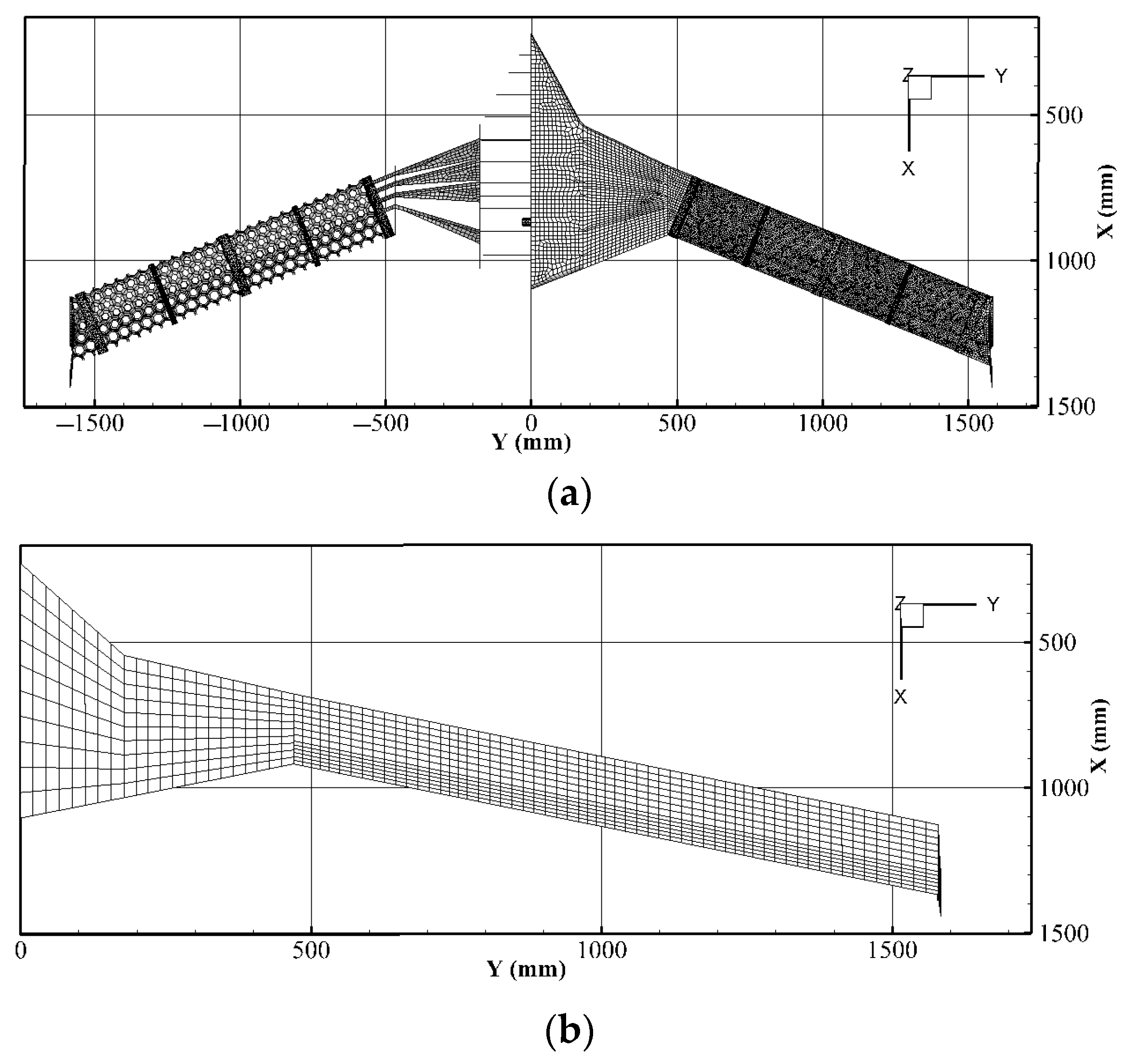
2.1. Structural and Aerodynamic Models

Similar to the UAV demonstrator designed by the University of Minnesota [28], a flying-wing layout aircraft is used for GLA control. The model has a root chord of 878 mm, a wingtip chord of 240 mm, and a half-span length of 1578 mm. For the convenience of 3D printing, the entire wing is made of ULTEM 9085 filament. Only the semi-span wind tunnel model is considered in this paper, and the corresponding NASTRAN finite element model (FEM) is shown in Figure 1a. The first six elastic mode shapes and natural frequencies of the wing clamped at the wing root are shown in Figure 2 and

Table 1. The first six natural frequencies of the clamped wing.

Mode	Frequency (Hz)	Mode Shape
1	2.39	1st vertical bending
2	14.32	2nd vertical bending
3	16.15	1st in-plane bending
4	22.87	1st torsion
5	26.45	2nd torsion
6	43.35	3rd vertical bending

, respectively.

In this study, the unsteady aerodynamic forces are computed using the Doublet Lattice Method (DLM), which is a subsonic model for harmonically oscillating lifting surfaces [29]. Figure 1b shows the aerodynamic model of the flying-wing aircraft, in which the lifting surface is represented by a number of aerodynamic boxes of trapezoidal shape.

2.2. State-Space Open-Loop Aeroservoelastic Equations

In the DLM aerodynamic model, the non-penetrating boundary condition is used to establish the relationship between the dimensionless downwash velocity and the harmonically oscillating lifting surface at the control points on the aerodynamic boxes. Then, the pressure coefficients on aerodynamic boxes can be calculated via the aerodynamic influence coefficient (AIC) matrix and dimensionless downwash velocity. Finally, a spline matrix is constructed to establish the data transfer relationship between the structural displacements at the finite element nodes and the displacements at the control points on the aerodynamic boxes. Using the equivalent principle of virtual work and introducing the modal coordinate transformation, one obtains the following aeroelastic equation expressed in the modal space:

$$M_{hh}\ddot{\xi }+D_{hh}\dot{\xi }+K_{\mathrm{hh}}\xi +M_{hc}\ddot{\delta }=q_d{Q}_{hh}\xi +q_d{Q}_{hc}\delta +q_d{Q}_{hg}\frac{w_g(t)}{U}$$

(1)

in which $M_{hh}$, $D_{hh}$, and $K_{hh}$ are modal mass, damping, and stiffness matrices, respectively. $M_{hc}$ is the mass coupling matrix. $Q_{hh}$, $Q_{hc}$, and $Q_{hg}$ are matrices of generalized aerodynamics force (GAF) due to structural motion, deflections of control surfaces, and gust disturbance, respectively.

In order to cast the aeroelastic equation of motion in a time-domain constant coefficient equation, the minimum state (MS) [30] approximation is used. It assumes that the frequency-domain aerodynamic matrices can be approximated as follows:

$$Q(k)=A_0+A_1\cdot \mathrm{i}k+A_2\cdot {(\mathrm{i}k)}^2+D_W{(\mathrm{i}k\cdot I-R_w)}^{-1}{E}_w\cdot \mathrm{i}k$$

(2)

where $Q=[\begin{array}{ccc}{Q}_{hh}& Q_{hc}& Q_{hg}\end{array}]$ is the GAF matrix. $R_w$ is the aerodynamic lag root matrix, and the other matrices are obtained by solving the least squares (LS) problem.

Using the MS approximation and introducing the additional aerodynamic states, the state-space open-loop aeroelastic equation can be written as [31]

$${\dot{x}}_{ae}=A_{ae}{x}_{ae}+B_{ae}{u}_{ae}+B_{aw}{\tilde{w}}_g$$

(3)

where the state vector $x_{ae}$ includes modal displacement $\xi$, modal velocity $\dot{\xi }$, and the aerodynamic states. $u_{ae}$ is the actual control surface deflection vector. The gust disturbance vector ${\tilde{w}}_g$ contains vertical gust velocity $w_g$ and its time derivative ${\dot{w}}_g$, namely ${\tilde{w}}_g={[\begin{array}{cc}{w}_g& {\dot{w}}_g\end{array}]}^{\mathrm{T}}$.

The dynamic model of the actuator driving the $i\mathrm{th}$ control surface is specified by a third-order transfer function, having the form

$${\delta }_i(s)=\frac{a_{0i}}{s^3+a_{2i}{s}^2+a_{1i}s+a_{0i}}{u}_{c,i}(s),i=1,2,\cdots , n_c$$

(4)

where $u_{ci}$ is the servo-commanded control surface deflection and ${\delta }_i$ is the actual deflection. Note that the DC ($s=0$) gain of the transfer function is one and is, thus, in steady state $u_{ac,i}={\delta }_i$.

The assembled actuator state space equation is, thus, cast in the following form:

$$\left\{\begin{array}{c}\dot{\delta }\\ \ddot{\delta }\\ \stackrel{⃛}{\delta }\end{array}\right\}=\left\{\begin{array}{ccc}0& I& 0\\ 0& 0& I\\ -A_{ac0}& -A_{ac1}& -A_{ac2}\end{array}\right\}\left\{\begin{array}{c}\delta \\ \dot{\delta }\\ \ddot{\delta }\end{array}\right\}+\left\{\begin{array}{c}0\\ 0\\ A_{ac0}\end{array}\right\}{u}_{ac},A_{aci}=\mathrm{diag}[a_{1i},\cdots ,a_{n_{c}i}]$$

(5)

or

$${\dot{x}}_{ac}=A_{ac}{x}_{ac}+B_{ac}{u}_{ac}$$

(6)

The augmentation of $x_{ae}$ in Equation (3) to include the actuator states $x_{ac}$ yields the following open-loop aeroelastic equation:

$${\dot{x}}_p=A_p{x}_p+B_p{u}_p+B_{pw}{\tilde{w}}_g$$

(7)

where

$$x_p=\left\{\begin{array}{c}{x}_{ae}\\ x_{ac}\end{array}\right\}, A_p=\left[\begin{array}{cc}{A}_{ae}& B_{ae}\\ 0& A_{ac}\end{array}\right], B_p=\left[\begin{array}{c}0\\ B_{ac}\end{array}\right], B_{pw}=\left[\begin{array}{c}{B}_{aw}\\ 0\end{array}\right], u_p=u_{ac}$$

(8)

The output equation is

$$y_p=C_p{x}_p+D_{aw}{\tilde{w}}_g$$

(9)

The output vector $y_p$ can be sensor readings, such as displacement, velocity, and acceleration responses at the specified finite element nodes, as well as the virtual load outputs, such as wing-root shear force, bending, and torsional moments. Equations (7) and (9) constitute the final open-loop aeroelastic equations of motion excited by control surface deflections and atmospheric gust. The purpose of GLA is to seek a control law that drives the control surfaces to deflect appropriately, thereby generating additional aerodynamic forces to minimize the outputs of the system.

3. Design of a MIMO Adaptive Feed-Forward Controller

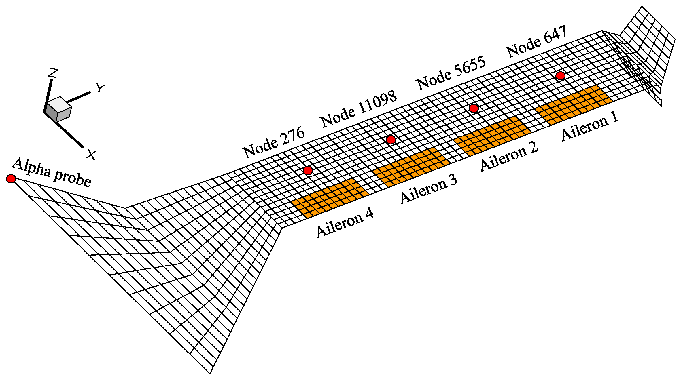
3.1. Control Surface and Sensor Layouts

The design of a MIMO feed-forward control system requires an appropriate reference signal that can provide the necessary disturbance information for controllers to calculate the control commands. This study assumes that there is an alpha probe at the aircraft nose available to measure the vertical gust velocity signal [32], as shown in Figure 3. Afterwards, the effective angle induced by gust can be computed from alpha probe measurements, which is used as the reference signal for feed-forward control.

In this study, a total of four control surfaces are used, and they are depicted in Figure 3, whose cut-off frequency is set as fifteen hertz. Four acceleration sensors located at nodes 647, 5655, 11098, and 276 are used to monitor the responses of the system. The output signals also include the incremental internal loads relative to the static equilibrium of the structure, which are not measured in the GLA control system and can be regarded as the virtual outputs of the system. In addition, acceleration signals at nodes 647 and 11098 are also employed to form the error signals in the subsequent adaptive feed-forward control design.

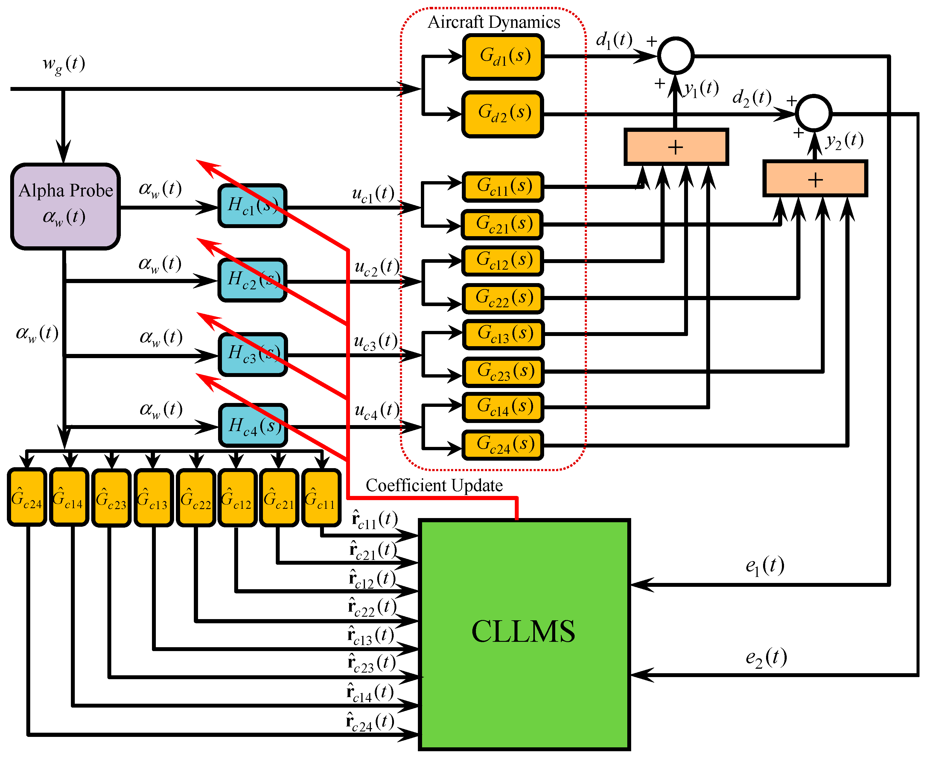
3.2. MIMO Adaptive Feed-Forward Control Scheme

Figure 3 illustrates the framework of the designed MIMO adaptive feed-forward control for GLA. Due to the high proportion of control surfaces in the span, two acceleration sensors at nodes 647 and 11098 are employed as error sensors. From the open-loop aeroelastic equation (see Equation (7)), we can see that both gust and control surface deflections can affect the outputs of the system. Therefore, the inputs of the system affect the outputs through two paths. The vertical gust velocity $w_g$ causes the acceleration responses $d_i$, $i=1,2$ at nodes 647 and 11098 via the primary path (PP) transfer function $G_{d1}(s)$ and $G_{d2}(s)$, respectively. From gust velocity measurements, the effective angle of attack ${\alpha }_w$ induced by gust can be calculated using $w_g/U$. Afterwards, the obtained reference signal ${\alpha }_w$ is fed forward to the adaptive controllers $H_{ci}(s)$ to generate the servo-commanded control surface deflections $u_{ci}$, $i=1\sim 4$. On the other hand, each control surface deflection $u_{ci}$ causes the outputs at nodes 647 and 11098 via the secondary path (SP) transfer function $G_{c1i}(s)$ and $G_{c2i}(s)$, respectively. Thus, the total signals $y_i$, $i=1,2$ are obtained by summing these accelerations due to these control surface deflections. The error signals at nodes 647 and 11098, denoted as $e_1(t)$ and $e_2(t)$, are formed by summing $d_i$ and $y_i$, $i=1,2$, respectively. In Figure 4, ${\widehat{G}}_{c1i}(s)$ and ${\widehat{G}}_{c2i}(s)$, as the estimated transfer functions of $G_{c1i}(s)$ and $G_{c2i}(s)$, respectively, are used to generate the filtered reference signals ${\widehat{r}}_{c1i}$ and ${\widehat{r}}_{c2i}$. The filtered reference signals together with the error signals are used to update the parameters of adaptive controllers. The objective of GLA control is to adjust the controller parameters to minimize the error signals as much as possible.

3.3. MIMO Adaptive Feed-Forward Control Algorithm

3.3.1. FIR Filter

The adaptive feed-forward controllers $H_{ci}(s)$, $i=1\sim 4$, are implemented by a set of digital filters. In this study, a finite impulse response (FIR) filter is used to construct the adaptive control law due to its prominent advantage in stability.

The transfer function of an FIR filter can be written as

$$H_{cj}(z)=h_{j,0}+h_{j,1}{z}^{-1}+\cdots +h_{j,N-1}{z}^{-(N-1)}, j=1,2,\cdots ,N_c$$

(10)

where $h_{j,0},\hspace{0.33em}{h}_{j,1},\hspace{0.33em}\cdots ,\hspace{0.33em}{h}_{j,N-1}$ are the weight coefficients of filter $j$, N is the order of the filter, and $N_c$ is the number of the controllers.

The feed-forward control command is generated by filtering a sampled version of the sensed gust-induced angle-of-attack signal ${\alpha }_w(t)$ via an FIR filter. Thus, the commanded deflection of a control surface $u_{cj}(n)$ at discrete time step $n$ can be written as

$$u_{cj}(n)={\alpha }^{\mathrm{T}}(n)h_{cj}(n)=h_{cj}^{\mathrm{T}}(n)\alpha (n), j=1,2,\cdots ,N_c$$

(11)

where the weight coefficient vector of the filter is

$$h_{cj}(n)={[\begin{array}{cccc}{h}_{j,0}(n)& h_{j,1}(n)& \cdots & h_{j,N-1}(n)\end{array}]}^{\mathrm{T}}$$

(12)

and the gust-induced angle-of-attack vector $\alpha (n)$ is defined as

$$\alpha (n)={[\begin{array}{cccc}{\alpha }_w(n)& {\alpha }_w(n-1)& \cdots & {\alpha }_w(n-N+1)\end{array}]}^{\mathrm{T}}$$

(13)

3.3.2. Adaptive Updating Law of the Weight Coefficients

As is well known, the LMS algorithm is widely used in the active control of vibration and noise due to its easy implementation and low computational cost. However, the LMS algorithm will encounter stability issues during long-term operation in a quantized digital computing environment. Specifically, the weight coefficients of the filter are prone to slowly drift, which will eventually lead to overflow. This drawback can be remedied by the leaky least mean squares (LLMS) algorithm, in which a leakage factor is introduced to suppress the weight-drift problem [33].

The cost function $J(n)$ in the LLMS algorithm can be written as

$$J(n)={\displaystyle \sum _{i=1}^{N_e}{e}_i^2(n)}+\gamma {\displaystyle \sum _{j=1}^{N_c}{h}_{cj}^{\mathrm{T}}(n)h_{cj}(n)}$$

(14)

where $\gamma \in (0,1)$ is the introduced leakage factor $\gamma$ that leaks the excessive energy associated with weight drift. $N_e$ is the number of the error signals ($N_e=2$ in this study). The error signals $e_i$ are defined as

$$e_i(n)=d_i(n)+y_i(n)=d_i(n)+{\displaystyle \sum _{j=1}^{N_c}{h}_{cj}^{\mathrm{T}}(n){\widehat{r}}_{cij}(n)}, i=1,2,\cdots ,N_e$$

(15)

where

$${\widehat{r}}_{cij}(n)={[\begin{array}{cccc}{\widehat{r}}_{cij}(n)& {\widehat{r}}_{cij}(n-1)& \cdots & {\widehat{r}}_{cij}(n-N+1)\end{array}]}^{\mathrm{T}}$$

(16)

The element ${\widehat{r}}_{cij}(n)$ is the output of the system ${\widehat{G}}_{cij}(s)$ at discrete time step $n$.

Substituting Equation (15) into Equation (14), the cost function is updated as follows

$$J(n)={{\displaystyle \sum _{i=1}^{N_e}\left(d_i(n)+{\displaystyle \sum _{j=1}^{N_c}{h}_{cj}^{\mathrm{T}}(n){\widehat{r}}_{cij}(n)}\right)}}^2+\gamma {\displaystyle \sum _{j=1}^{N_c}{h}_{cj}^{\mathrm{T}}(n)h_{cj}(n)}$$

(17)

Differentiating this with respect to the $j\mathrm{th}$ weight coefficient vector $h_{cj}$ gives

$$\begin{array}{l}\frac{\partial J(n)}{\partial h_{cj}(n)}={\displaystyle \sum _{i=1}^{N_e}\frac{\partial e_i^2(n)}{\partial h_{cj}(n)}}+\gamma {\displaystyle \sum _{j=1}^{N_c}\frac{\partial (h_{cj}^{\mathrm{T}}(n)h_{cj}(n))}{\partial h_{cj}(n)}}\\ \hspace{1em}\hspace{1em}=2{\displaystyle \sum _{i=1}^{N_e}{\widehat{r}}_{cij}(n)\cdot e_i}+2\gamma h_{cj}(n)\end{array}$$

(18)

The gradient descent algorithm yields the following weight updating law

$$h_{cj}(n+1)=h_{cj}(n)-\mu \left(2{\displaystyle \sum _{i=1}^{N_e}{\widehat{r}}_{cij}(n)\cdot e_i}+2\gamma h_{cj}(n)\right)$$

(19)

or

$$h_{cj}(n+1)=(1-\mu \gamma )h_{cj}(n)-\mu {\displaystyle \sum _{i=1}^{N_e}{\widehat{r}}_{cij}(n)\cdot e_i}$$

(20)

where $\mu$ is the convergence coefficient. For simplicity, coefficient 2 is omitted in Equation (20).

However, the obtained weights will produce a biased estimate of the Wiener solution in the LLMS algorithm. As an improved version of the LLMS algorithm, the CLLMS algorithm used in this study can ensure an unbiased estimate of the filter coefficients [34]. In the CLLMS algorithm, the updating rules for the weight coefficients of the filter can be written as

$$h_{cj}(n+1)={\overline{h}}_{cj}(n)-\mu {\displaystyle \sum _{i=1}^{N_e}{\widehat{r}}_{cij}(n)\cdot e_i}$$

(21)

where

$${\overline{h}}_{cj}(n)=\left\{\begin{array}{ll}{\overline{\overline{h}}}_{cj}(n),\hfill & \mathrm{if}\hspace{0.33em}\left|h_{j,k}(n)\right|\ge C_1\hfill \\ h_{cj}(n),\hfill & \mathrm{otherwise}\hfill \end{array}\right.$$

(22)

$${\overline{\overline{h}}}_{cj}(n)=\left\{\begin{array}{c}{h}_{j,0}(n)\\ ⋮\\ \left(1-\mu {\gamma }_c(n,h_{j,k}(n))\right)h_{j,k}(n)\\ ⋮\\ h_{j,N-1}(n)\end{array}\right\}$$

(23)

with $k=\mathrm{mod}(n,N)$, satisfying $|h_{j,k}(n)|\ge C_1$. The leakage factor ${\gamma }_c$ is calculated by

$${\gamma }_c(n,h_{j,k}(n))=\left\{\begin{array}{ll}\gamma ,\hfill & \mathrm{if}\hspace{0.33em}\left|h_{j,k}(n)\right|\ge C_2\hfill \\ \gamma -\frac{\gamma }{2}{\left(\frac{C_2-\left|h_{j,k}(n)\right|}{D}\right)}^2,\hfill & \mathrm{if}\hspace{0.33em}{C}_1+D\le \left|h_{j,k}(n)\right|<C_2\hfill \\ \frac{\gamma }{2}{\left(\frac{\left|h_{j,k}(n)\right|-C_1}{D}\right)}^2,\hfill & \mathrm{if}\hspace{0.33em}{C}_1\le \left|h_{j,k}(n)\right|<C_1+D\hfill \\ 0,\hfill & \mathrm{otherwise}\hfill \end{array}\right.$$

(24)

where $D=(C_2-C_1)/2$, $C_1$, and $C_2$ are the positive constants satisfying $C_1<C_2$. Note that the CLLMS algorithm requires four constants: $\mu$, $\gamma$, $C_1$, and $C_2$ [34].

4. Numerical Simulations for GLA Control of the Flying Wing

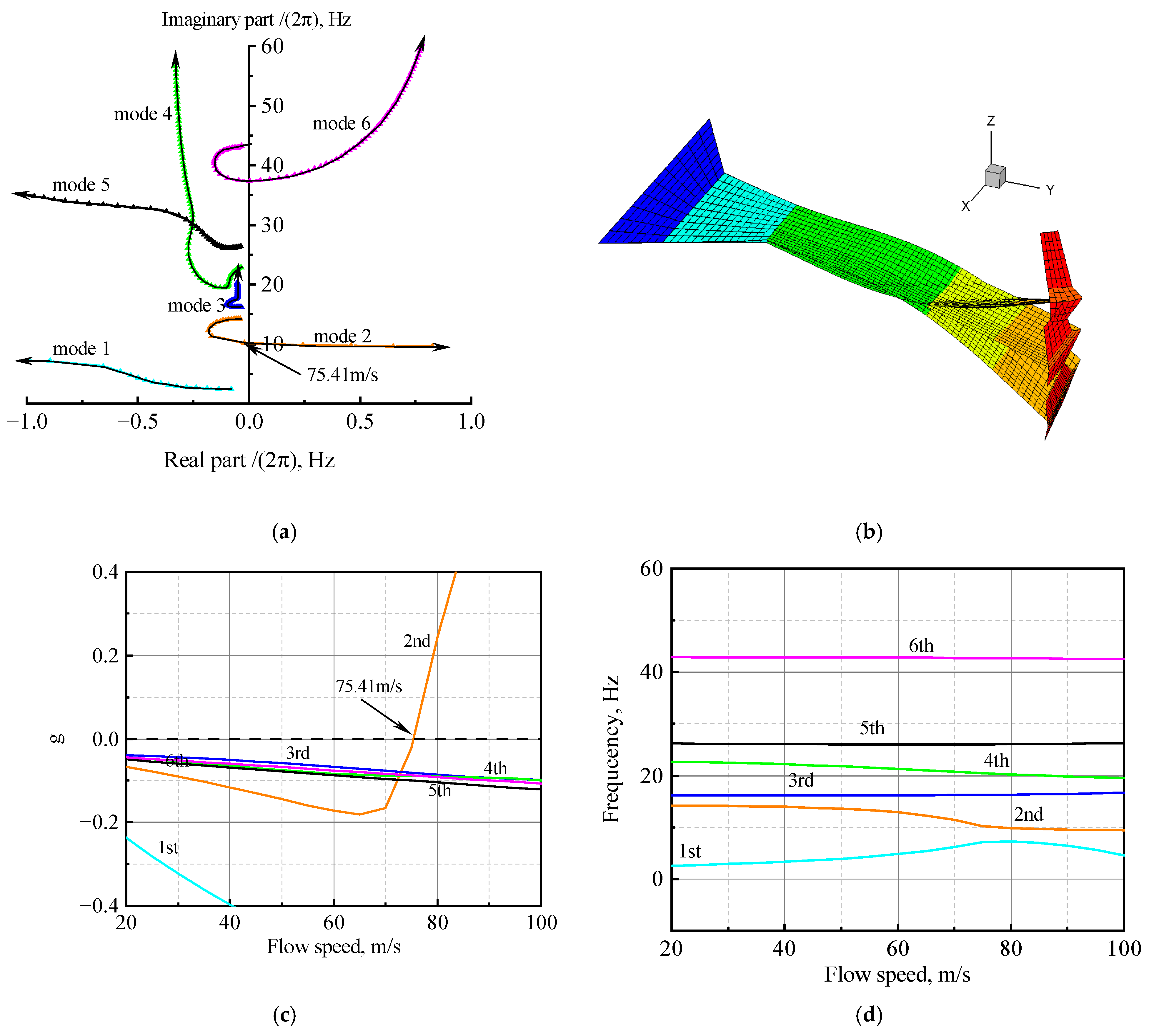
4.1. Flutter Analysis

In order to ensure that the subsequent GLA simulations can be performed within the safe flight envelope, flutter analysis of the flying wing is carried out by tracing the eigenvalues of the system matrix $A_p$ in Equation (7) at different flow speeds. Figure 5a shows a root locus diagram of the system matrix $A_p$, in which each arrow indicates the direction of an increase in flow speed. It can be seen that, as the flow speed increases, the second-order mode passes through the imaginary axis and becomes unstable first. The eigenvalue with zero real part on the mode 2 branch is a critical point, at which the flutter speed is found to be 75.41 m/s with a flutter frequency of 10.1 Hz. Figure 5b illustrates that the flutter shape is primarily a superposition of the second vertical bending and the first torsional modes. The V-g and V-f diagrams obtained from frequency-domain flutter analysis are also shown in Figure 5c,d.

4.2. Simulation Environment for GLA Control

After flutter analysis is completed, GLA control simulations can be carried out. Figure 6 illustrates a simulation block diagram of the adaptive feed-forward GLA control system. The feed-forward controller utilizes three different types of signals, namely acceleration error signals $e_i(n)$, filtered reference signals ${\widehat{r}}_{cij}(n)$, and the gust-induced angle-of-attack vector $\alpha (n)$, to generate deflection commands of control surfaces. The adaptive controller is implemented using a level-2 S-function in the MATLAB R2018a Simulink platform. First, the time-series vector $\alpha (n)$ is constructed by the sensed gust-induced angle-of-attack signal ${\alpha }_w(n)$. Afterwards, the weight coefficients of each FIR filter are updated. Finally, the commanded control surface deflections at discrete time step $n$ are generated and used as the outputs of the level-2 S-function.

Since GLA control always operates below the flutter speed of the system, all numerical simulations are performed at a cruise speed of 27.2 m/s and sea level. The continuous gust scale in the Dryden model introduced in Section 4.3 is set to $L_w=53.3\hspace{0.33em}\mathrm{m}$, and the RMS value of the gust velocity is taken as ${\sigma }_w=0.5\hspace{0.33em}\mathrm{m}/\mathrm{s}$. The time history of gust velocity for the Dryden gust model is generated using a shaped filter excited by white noise. In Simulink simulations, the sampling period is taken as 0.001 s. The order of the FIR filter for each adaptive controller is set as N = 42. When the GLA control system is activated, the filter coefficients are updated online by the CLLMS algorithm, in which the convergence coefficient is $\mu =0.005$, leakage factor is $\gamma =0.5$, and constants C₁ and C₂ are taken as 0.5 and 0.7, respectively.

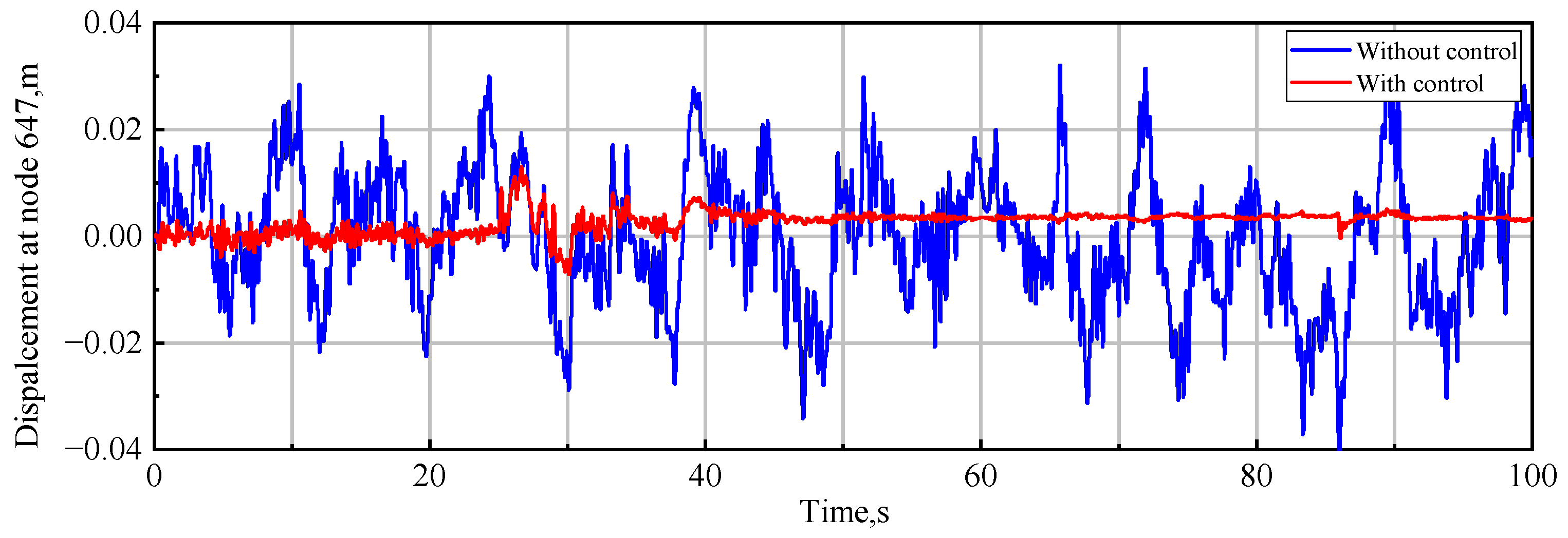
4.3. GLA Control in a Continuous Dryden Gust Field

The widely used standard gust models can be divided into two categories: continuous gusts and discrete gusts. The former employs a statistical approach to describe the gust disturbance, including two standard forms: Dryden gust and von Karman gust. In this study, the Dryden model is used because it can be represented as a rational function form and it is easier to obtain a realization in the time domain. The power spectral density (PSD) of vertical gust velocity in the Dryden model can be written as [35]

$${\mathsf{\Phi }}_w(\omega )={\sigma }_w^2\frac{{\tau }_w}{\mathsf{\pi }}\frac{1+3{(\omega {\tau }_w)}^2}{{[1+{(\omega {\tau }_w)}^2]}^2}$$

(25)

where ${\tau }_w=L_w/U$, and $L_w$ are the gust scale. ${\sigma }_w$ represents the root-mean-square (RMS) value of the gust velocity. $\omega$ is the angular frequency.

In order to perform time-domain simulations, Dryden gust can be expressed in the following state-space form

$${\dot{x}}_g(t)=A_g{x}_g(t)+B_{g}r(t)$$

(26)

$${\tilde{w}}_g(t)=C_g{x}_g(t)$$

(27)

where

$$x_g(t)=\left\{\begin{array}{c}{x}_g(t)\\ {\dot{x}}_g(t)\\ {\overline{x}}_g(t)\end{array}\right\}, {\tilde{w}}_g(t)=\left\{\begin{array}{c}{w}_g(t)\\ {\dot{w}}_g(t)\end{array}\right\}, A_g=\left[\begin{array}{ccc}0& 1& 0\\ -{\tau }_w^{-2}& -2{\tau }_w^{-1}& a\\ 0& 0& -a\end{array}\right]$$

(28)

$$B_g=\left[\begin{array}{c}0\\ 0\\ {\sigma }_w/\sqrt{\mathsf{\pi }}\end{array}\right], C_g=\left[\begin{array}{ccc}{\tau }_w^{-3/2}& \sqrt{3}{\tau }_w^{-1/2}& 0\\ -\sqrt{3}{\tau }_w^{-5/2}& (1-2\sqrt{3}){\tau }_w^{-3/2}& a\sqrt{3}{\tau }_w^{-1/2}\end{array}\right]$$

(29)

where $a$ is the cut-off frequency of the low-pass filter. $r(t)$ is the Gaussian white noise input. Dryden gust distribution experienced by the wing is shown in Figure 7.

The simulation parameters in the Dryden gust condition are shown in Section 4.2. Figure 8 shows the convergence behaviors of the selected weight coefficients of an FIR controller during the training process. The initial values of the FIR filter coefficients are all set to zero. Obviously, a converged controller is obtained at $t$ = 870 s. The converged coefficients still exhibit oscillations around their average values due to the stochastic nature of the gust disturbance and instantaneous approximation of the gradient of cost function during the weight updating.

In simulations, Dryden gust velocity and its first derivative with respect to time are computed using Equations (26) and (27). Subsequently, the trained CLLMS controller is employed to verify the effectiveness of GLA control in the Dryden gust condition. Figure 9 illustrates the acceleration responses at the monitoring nodes when the flying wing equipped with a GLA system travels through the Dryden gust field. Obviously, the GLA control can effectively suppress vibrations at the monitoring nodes on the wing. As shown in Figure 10, after activating the GLA control, the wing-root loads are significantly reduced. The actual deflections of control surfaces, namely the outputs of actuators, are shown in Figure 11.

The statistical results in

Table 2. Performance of the CLLMS-based adaptive feed-forward control system (Dryden gust).

Parameter	RMS Reduction	Parameter	RMS Reduction
$N_{z647}$, ${\mathrm{m}/\mathrm{s}}^2$	80.98%	$N_{z11098}$, ${\mathrm{m}/\mathrm{s}}^2$	46.62%
$N_{z5655}$, ${\mathrm{m}/\mathrm{s}}^2$	65.63%	$N_{z276}$, ${\mathrm{m}/\mathrm{s}}^2$	34.44%
$F_z$, $\mathrm{N}$	66.12%	$M_x$, $\mathrm{Nm}$	80.72%
$M_y$, $\mathrm{Nm}$	94.14%	⸺	⸺

indicate that the error signals, RMS values of the accelerations at monitoring nodes, and wing-root internal loads are significantly reduced. For example, an 80.72% reduction in the RMS value of the wing-root bending moment is achieved. This is of great significance for the weight reduction design of the aircraft. The GLA results demonstrate that the designed CLLMS-based controllers are very effective.

It is noted that a set of time–history curves cannot easily be used to simultaneously display the correlations of the GLA performances between two physical quantities. This issue can be remedied by plotting a convex hull diagram about two physical variables [36]. First, the gust-induced response data for a set of physical quantities are computed by open- and closed-loop simulations, respectively. Then, the discrete points corresponding to two selected physical quantities are plotted on a two-dimensional plane. Finally, a convex hull is formed by the minimum convex polygon, which encompasses all these discrete points. The correlations of GLA performance between two selected physical quantities are clearly demonstrated in Figure 12.

4.4. GLA Control in a Discrete Gust Field

When an aircraft travels through the 1-cos gust field with a cruise speed $U$, the vertical disturbance velocity sensed by the gust reference point on the aircraft is given by

$$w_g(t)=\left\{\begin{array}{cc}\frac{{\overline{w}}_g}{2}(1-\cos 2\mathsf{\pi }{f}_{g}t),\hfill & \hfill \hspace{0.33em}0\le t\le \frac{L_g}{U}\\ 0,\hfill & \hfill t>\frac{L_g}{U}\end{array}\right.$$

(30)

where ${\overline{w}}_g$ is the amplitude of gust velocity, $L_g$ is the gust scale, and $f_g=U/L_g$ is the gust excitation frequency.

The aim of this subsection is to verify whether the converged CLLMS-based controllers trained in the continuous gust environment are also applicable in the case of a discrete gust condition. In simulations, the maximum gust velocity ${\overline{w}}_g$ and the gust excitation frequency $f_g$ are taken as 1 m/s and 3 Hz, respectively. The alleviation results for acceleration and wing-root internal load responses are shown in Figure 13 and Figure 14, respectively. It can be observed that the responses of the flying-wing system are significantly reduced after applying the GLA control. It can be seen from Figure 15 that among all control surfaces, aileron 4 has the largest deflection amplitude because the outermost control surface has the highest effectiveness in suppressing bending vibration response.

Table 3. Performance of the CLLMS-based adaptive feed-forward control system (1-cos gust).

Parameter	Reduction of the Maximum Value	Parameter	Reduction of the Maximum Value
$N_{z647}$, ${\mathrm{m}/\mathrm{s}}^2$	83.10%	$N_{z11098}$, ${\mathrm{m}/\mathrm{s}}^2$	73.23%
$N_{z5655}$, ${\mathrm{m}/\mathrm{s}}^2$	90.12%	$N_{z267}$, ${\mathrm{m}/\mathrm{s}}^2$	70.72%
$M_x$, $\mathrm{Nm}$	77.59%	$F_z$, $\mathrm{N}$	62.16%

gives a summary of the GLA performance in the 1-cos gust condition. It is, thus, clear that the CLLMS-based controllers trained in the continuous gust condition still maintain good performance in the discrete gust environment.

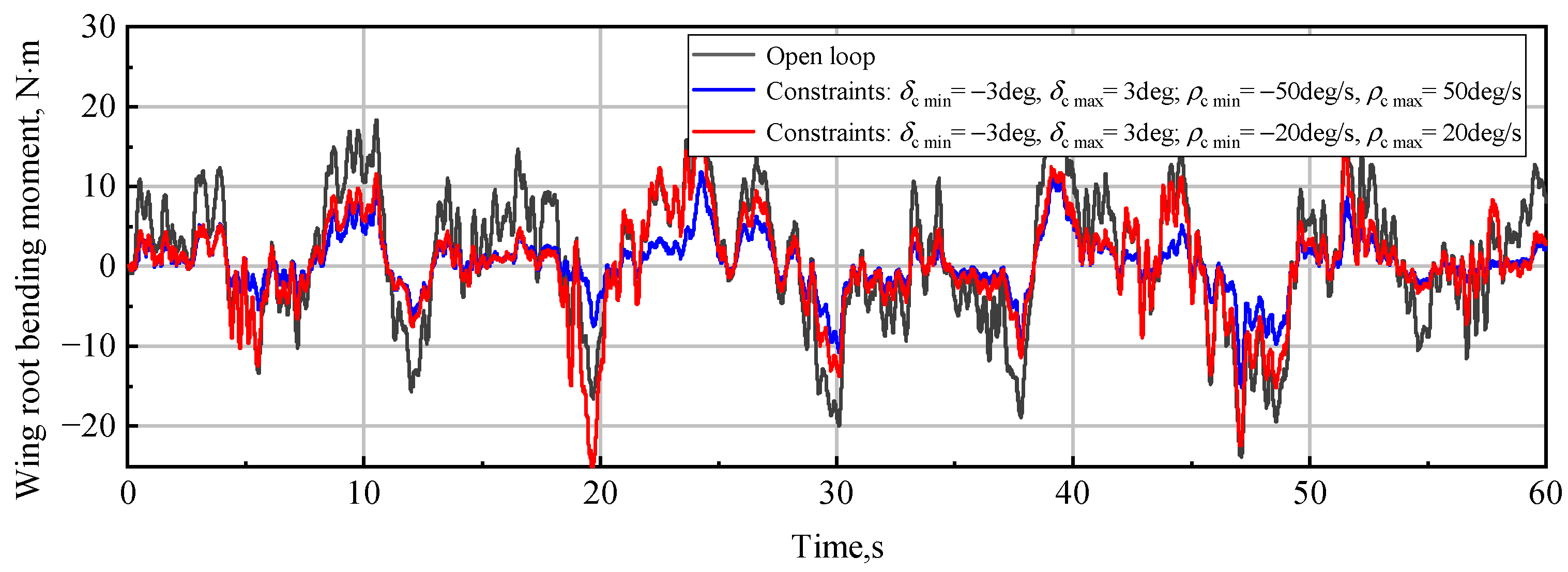
4.5. Constraints on Control Surface Deflections

Note that the effort constraints are not involved in the above control algorithm. In practical applications, the total power of the control signal is limited because the actuator has limited driving capability. In addition, when incorporating GLA control into a flight control system, it is necessary to limit the deflection of the control surface. To this end, assume that the deflection angle ${\delta }_c(t)$ and the deflection rate ${\dot{\delta }}_c(t)$ of a control surface are bounded by:

$$\left\{\begin{array}{c}{\delta }_{c\min }\le {\delta }_c(t)\le {\delta }_{c\max }\\ {\rho }_{c\min }\le {\dot{\delta }}_c(t)\le {\rho }_{c\max }\end{array}\right.$$

(31)

where ${\delta }_{c\min }$ and ${\delta }_{c\max }$ represent the minimum and maximum allowed deflections, respectively. ${\rho }_{c\min }$ and ${\rho }_{c\max }$ represent the minimum and maximum allowed deflection rates, respectively.

Let $T$ be the sampling interval. Using the definition of time derivative, Equation (31) can be transformed into the following form:

$${\underset{\_}{\delta }}_c(t)\le {\delta }_c(t)\le {\overline{\delta }}_c(t)$$

(32)

where

$$\left\{\begin{array}{c}{\underset{\_}{\delta }}_c(t)=\max \{{\delta }_{c\min },{\delta }_c(t-T)+T{\rho }_{c\min }\}\\ {\overline{\delta }}_c(t)=\min \{{\delta }_{c\max },{\delta }_c(t-T)+T{\rho }_{c\max }\}\end{array}\right.$$

(33)

In this paper, an algorithm for bounding the controller output is given by the following coefficient update and control output equations:

• If $u_c(n)>{\overline{\delta }}_c(t)$

  $$\left\{\begin{array}{c}{h}_c(n+1)=h_c(n+1)\frac{{\overline{\delta }}_c(n)}{u_c(n)}\\ u_c(n)=u_c(n)\frac{{\overline{\delta }}_c(n)}{u_c(n)}={\overline{\delta }}_c(n)\end{array}\right.$$
• If $u_c(n)\le {\underset{\_}{\delta }}_c(t)$

  $$\left\{\begin{array}{c}{h}_c(n+1)=h_c(n+1)\frac{{\underset{\_}{\delta }}_c(n)}{u_c(n)}\\ u_c(n)=u_c(n)\frac{{\underset{\_}{\delta }}_c(n)}{u_c(n)}={\underset{\_}{\delta }}_c(n)\end{array}\right.$$

  where $u_c(n)$ is the controller output, namely the command control surface deflection.

To verify the effectiveness of the above weight-updating rules, first, the deflection angle for each aileron is bounded by $\pm 3.0\hspace{0.17em}\hspace{0.17em}\mathrm{deg}$, and the deflection rate is bounded by $\pm 50\hspace{0.17em}\hspace{0.17em}\mathrm{deg}/\mathrm{s}$. From the solid red line in Figure 16 and Figure 17, the algorithm does limit the deflection angle of aileron 1. The algorithm did not affect the deflection rate because it did not exceed the amplitude of the constraint. Constraints on deflection motion will result in the degradation of GLA performance, as illustrated in Figure 18.

Table 4. Performance of the adaptive feed-forward control system with constraint on amplitude of defection (${\delta }_{c\min }=-3.0\hspace{0.17em}\mathrm{deg}, {\delta }_{c\max }=3.0\hspace{0.17em}\mathrm{deg}; {\rho }_{c\min }=-50\hspace{0.17em}\mathrm{deg}/\mathrm{s}, {\rho }_{c\max }=50\hspace{0.17em}\mathrm{deg}/\mathrm{s}$.

Parameter	RMS Reduction with Constraint (without)	Parameter	RMS Reduction with Constraint (without)
$N_{z647}$, ${\mathrm{m}/\mathrm{s}}^2$	61.35% (80.98%)	$N_{z11098}$, ${\mathrm{m}/\mathrm{s}}^2$	30.87% (46.62%)
$N_{z5655}$, ${\mathrm{m}/\mathrm{s}}^2$	48.38% (65.63%)	$N_{z276}$, ${\mathrm{m}/\mathrm{s}}^2$	19.27% (34.44%)
$F_z$, $\mathrm{N}$	55.08% (66.12%)	$M_x$, $\mathrm{Nm}$	58.77% (80.72%)
$M_y$, $\mathrm{Nm}$	65.94% (94.14%)	⸺	⸺

lists the percentage of RMS reduction under the constraint of the amplitude of defection angle.

Furthermore, in order to study the GLA performance when the deflation rate reaches saturation, the deflection angle for each aileron is bounded by $\pm 3.0\hspace{0.17em}\mathrm{deg}$, and the deflection rate is bounded by $\pm 20\hspace{0.17em}\mathrm{deg}/\mathrm{s}$, which means the fast rate of the deflection is constrained. As illustrated in Figure 19 and Figure 20, the algorithm takes account of both amplitude and rate constraints. Figure 21 shows that the performance of the load reduction deteriorates compared with the unsaturation situation of the deflection rate.

Table 5. Performance of the adaptive feed-forward control system with constraints on amplitude and rate of defection (${\delta }_{c\min }=-3.0\hspace{0.17em}\mathrm{deg}, {\delta }_{c\max }=3.0\hspace{0.17em}\mathrm{deg}; {\rho }_{c\min }=-20\hspace{0.17em}\mathrm{deg}/\mathrm{s}, {\rho }_{c\max }=20\hspace{0.17em}\mathrm{deg}/\mathrm{s}$.

Parameter	RMS Reduction with Constraints (without)	Parameter	RMS Reduction with Constraints (without)
$N_{z647}$, ${\mathrm{m}/\mathrm{s}}^2$	22.80% (80.98%)	$N_{z11098}$, ${\mathrm{m}/\mathrm{s}}^2$	14.15% (46.62%)
$N_{z5655}$, ${\mathrm{m}/\mathrm{s}}^2$	19.78% (65.63%)	$N_{z276}$, ${\mathrm{m}/\mathrm{s}}^2$	8.22% (34.44%)
$F_z$, $\mathrm{N}$	23.99% (66.12%)	$M_x$, $\mathrm{Nm}$	28.27% (80.72%)
$M_y$, $\mathrm{Nm}$	31.43% (94.14%)	⸺	⸺

lists the percentages of RMS reduction under the constraints of the amplitude and rate of defection. The reduction is only 28.27% and 31.43% in wing-root bending moment and torsional moment, respectively. It can be seen that the deflection motion constraints have a significant impact on GLA performance.

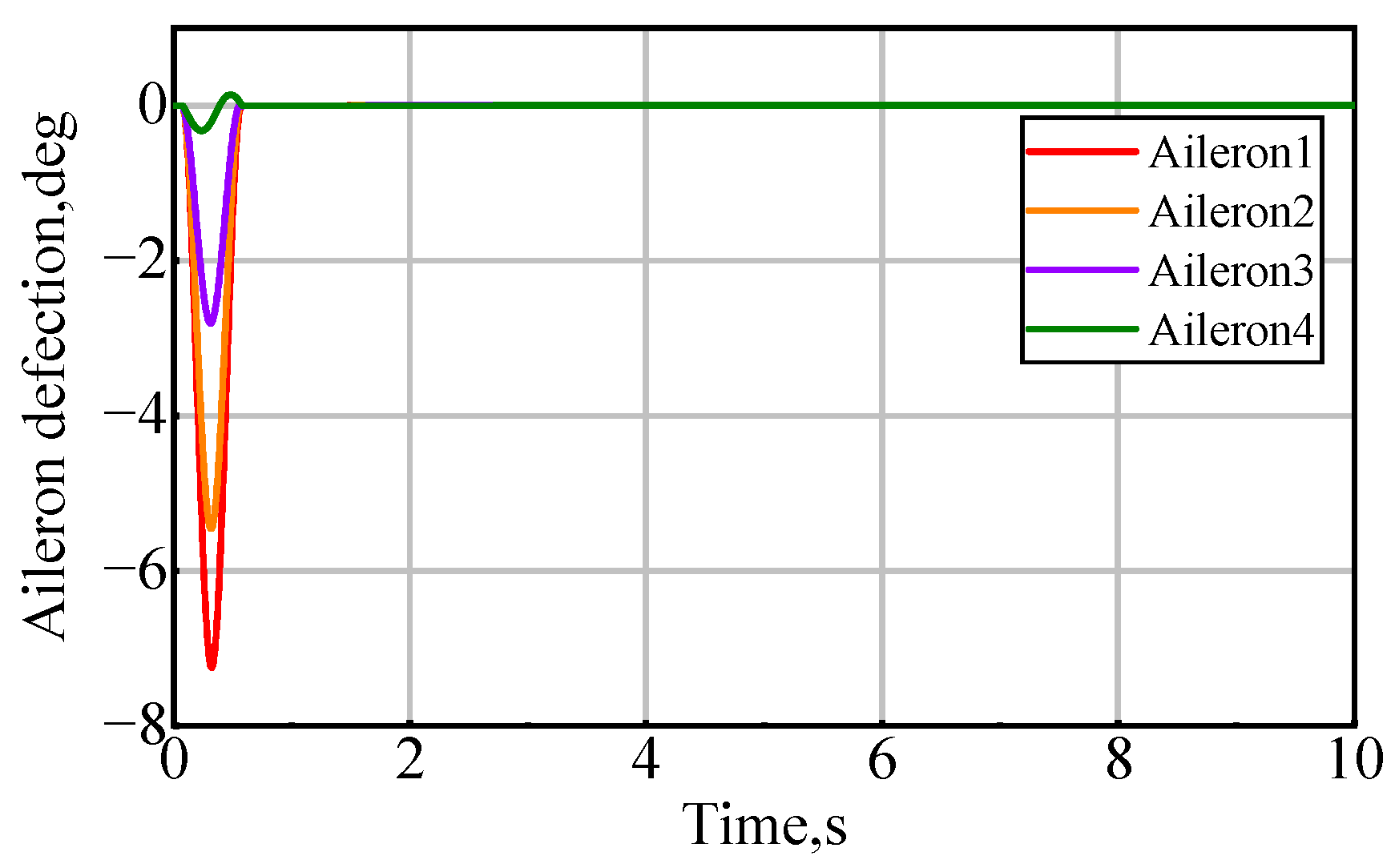
4.6. Case of Partial Failure of Actuators

The actuator has several failure modes, in which the control surface jamming is the most common failure mode. This subsection focuses on the influence of the jamming failure of the outmost control surface (aileron 1) on the GLA performance.

We assume that at the 25th second after GLA control is activated, aileron 1 is jammed at the 2 deg position; see the blue solid line in Figure 22. It can be seen that when aileron 1 fails suddenly, the deflection amplitudes of the other control surfaces gradually increase to compensate for the adverse effects resulting from aileron 1 failure. This indicates that the proposed MIMO adaptive feed-forward control has the self-regulating function for control energy in the case of jamming failure on the control surface. Figure 23 shows the displacement response at node 647 in the case of aileron 1 jamming failure. Before 25 s, the wing-tip displacement is significantly suppressed. Between 25 s and 40 s, the controller begins to adapt to this new fault environment. In this adaptation stage, there is a partial degradation of GLA performance. After 40 s, good GLA performance is restored. Since aileron 1 is jammed at the 2-degree position, a constant static displacement is found, As shown in Figure 23. It can be seen that the utilization of multiple control surfaces for GLA is beneficial for maintaining a stable GLA performance when actuator failure occurs. This is attributed to the robustness brought about by multiple control surfaces and the adaptability of the control algorithm.

5. Conclusions

To investigate the GLA problem for a flying-wing model with multiple control surfaces, this paper proposed a MIMO adaptive control scheme based on the CLLMS algorithm. The simulation results demonstrate that the developed GLA control system can significantly reduce accelerations at the monitoring nodes and wing-root internal loads in both continuous and discrete gust environments. The controllers trained in the continuous gust environment can also exhibit good performance in the discrete gust condition, because continuous gust can provide rich sample data for controller training.

Due to the limited power of the actuator, it is meaningful to impose constraints on the deflection angle and rate of the control surface during controller design. To this end, this paper proposed a weight-updating algorithm with constraints on the deflation angle and rate of control surface, and its effectiveness was verified through simulations. It was found that strict deflection constraints (e.g., very small deflection angle and rate) lead to a significant degradation in GLA performance. Finally, the influence of the actuator fault on GLA performance was studied in the event of the jamming failure occurring in the outmost control surface. The results show that the utilization of multiple control surfaces combined with the adaptive algorithm exhibits a good robustness to the actuator fault.

References

1. Barnaby, R.S. Gust pre-sensing devices for aircraft gust-alleviation systems. J. Frankl. Inst. 1955, 259, 459–462. [Google Scholar] [CrossRef]
2. Fournier, H.; Massioni, P.; Minh, T.P.; Bako, L.; Vernay, R.; Colombo, M. Robust gust load alleviation of flexible aircraft equipped with lidar. J. Guid. Control. Dynam. 2022, 45, 57–72. [Google Scholar] [CrossRef]
3. Hoblit, F.M. Gust Loads on Aircraft: Concepts and Applications; American Institute of Aeronautics and Astronautics, Inc.: Washington, DC, USA, 1988. [Google Scholar] [CrossRef]
4. Abdelmoula, F. Design of an open-loop gust alleviation control system for airborne gravimetry. Aerosp. Sci. Technol. 1999, 3, 379–389. [Google Scholar] [CrossRef]
5. Regan, C.D.; Jutte, C.V. Survey of Applications of Active Control Technology for Gust Alleviation and New Challenges for Lighter-Weight Aircraft; NASA/TM–2012-216008; Dryden Flight Research Center: Edwards, CA, USA, 2012. [Google Scholar]
6. Britt, R.T.; Jacobson, S.B.; Arthurs, T.D. Aeroservoelastic analysis of the B-2 bomber. J. Aircr. 2000, 37, 745–752. [Google Scholar] [CrossRef]
7. Scott, R.; Coulson, D.; Castelluccio, M.; Heeg, J. Aeroservoelastic wind-tunnel tests of a free-flying, joined-wing Sensorcraft model for gust load alleviation. In Proceedings of the 52nd AIAA/ASME/ASCE/AHS/ASC Structures, Structural Dynamics, and Materials Conference, Denver, CO, USA, 4–7 April 2011; American Institute of Aeronautics and Astronautics: Reston, VA, USA, 2011. [Google Scholar] [CrossRef]
8. Dillsaver, M.J.; Cesnik, C.E.S.; Kolmanovsky, I.V. Gust load alleviation control for very flexible aircraft. In Proceedings of the AIAA Atmospheric Flight Mechanics Conference, Portland, OR, USA, 8–11 August 2011; American Institute of Aeronautics and Astronautics: Reston, VA, USA, 2011. [Google Scholar] [CrossRef]
9. Yue, C.Y.; Zhao, Y.H. Active disturbance rejection controller design for alleviation of gust-induced aeroelastic responses. Aerosp. Sci. Technol. 2023, 133, 108116. [Google Scholar] [CrossRef]
10. Alam, M.; Hromcik, M.; Hanis, T. Active gust load alleviation system for flexible aircraft: Mixed feedforward/feedback approach. Aerosp. Sci. Technol. 2015, 41, 122–133. [Google Scholar] [CrossRef]
11. Hamada, Y.; Kikuchi, R.; Inokuchi, H. LIDAR-based Gust alleviation control system: Obtained results and flight demonstration plan. IFAC-PapersOnLine 2020, 53, 14839–14844. [Google Scholar] [CrossRef]
12. Sleeper, R.K. Spanwise Measurements of Vertical Components of Atmospheric Turbulence; NASA: Washington, DC, USA; Langley Research Center Hampton: Hampton, VA, USA, 1990. [Google Scholar]
13. Fuller, C.; Elliott, S.; Nelson, P. Active Control of Vibration; Academic Press: London, UK, 1996. [Google Scholar]
14. Wildschek, A. An Adaptive Feed-Forward Controller for Active Wing Bending Vibration Alleviation on Large Transport Aircraft. Ph.D. Dissertation, Technical University of Munich, Munich, Germany, 2008. [Google Scholar]
15. Brosilow, C.; Joseph, B. Techniques of Model-Based Control; Prentice Hall: Hoboken, NJ, USA, 2002. [Google Scholar]
16. Zhou, Q.; Li, D.; Ronch, A.D.; Chen, G.; Li, Y. Computational fluid dynamics-based transonic flutter suppression with control delay. J. Fluid. Struct. 2016, 66, 183–206. [Google Scholar] [CrossRef]
17. Wang, Y.; Ronch, A.D.; Maryam, G. Adaptive feedforward control for gust-induced aeroelastic vibrations. Aerospace 2018, 5, 86–104. [Google Scholar] [CrossRef]
18. Wildschek, A.; Maier, R.; Hoffmann, F.; Jeanneau, M.; Baier, H. Active wing load alleviation with an adaptive feed-forward control algorithm. In Proceedings of the AIAA Guidance, Navigation, and Control Conference, Keystone, CO, USA, 21–24 August 2006; American Institute of Aeronautics and Astronautics: Reston, VA, USA, 2006. [Google Scholar] [CrossRef]
19. Wildschek, A.; Maier, R.; Hahn, K.-U.; Leissling, D.; Press, M.; Zach, A. Flight test with an adaptive feed-forward controller for alleviation of turbulence excited wing bending vibrations. In Proceedings of the AIAA Guidance, Navigation, and Control Conference, Chicago, IL, USA, 10–13 August 2009; American Institute of Aeronautics and Astronautics: Reston, VA, USA, 2009. [Google Scholar] [CrossRef]
20. Wildschek, A.; Bartosiewicz, Z.; Mozyrska, D. A multi-input multi-output adaptive feed-forward controller for vibration alleviation on a large blended wing body airliner. J. Sound Vib. 2014, 333, 3859–3880. [Google Scholar] [CrossRef]
21. Widrow, B.; Stearns, S. Adaptive Signal Processing; Prentice-Hall: Hoboken, NJ, USA, 1985. [Google Scholar]
22. Hansen, C.H.; Snyder, S.D. Active Control of Noise and Vibration; CRC Press: London, UK, 2012. [Google Scholar]
23. Tobias, O.J.; Seara, R. Leaky delayed LMS algorithm: Stochastic analysis for Gaussian data and delay modeling error. IEEE Trans. Signal Process. 2004, 52, 1596–1606. [Google Scholar] [CrossRef]
24. Zhao, Y.H.; Yue, C.Y.; Hu, H.Y. Gust load alleviation on a large transport airplane. J. Aircr. 2016, 53, 1932–1946. [Google Scholar] [CrossRef]
25. Stanford, B.K. Optimal aircraft control surface layouts for maneuver and gust load alleviation. In Proceedings of the AIAA Scitech 2020 Forum, Orlando, FL, USA, 6–10 January 2020; American Institute of Aeronautics and Astronautics: Reston, VA, USA, 2020. [Google Scholar] [CrossRef]
26. Ricci, S.; De Gaspari, A.; Riccobene, L.; Fonte, F. Design and wind tunnel test validation of gust load alleviation systems. In Proceedings of the 58th AIAA/ASCE/AHS/ASC Structures, Structural Dynamics, and Materials Conference, Grapevine, TX, USA, 9–13 January 2017; American Institute of Aeronautics and Astronautics: Reston, VA, USA, 2017. [Google Scholar] [CrossRef]
27. Berg, J.; Ting, K.Y.; Mundt, T.J.; Mor, M.; Livne, E.; Morgansen, K.A. Exploratory wind tunnel gust alleviation tests of a multiple-flap flexible wing. In Proceedings of the AIAA SCITECH 2022 Forum, San Diego, CA, USA, 3–7 January 2022; American Institute of Aeronautics and Astronautics: Reston, VA, USA, 2022. [Google Scholar] [CrossRef]
28. Kotikalpudi, A.; Danowsky, B.P.; Schmidt, D.; Theis, J.; Seiler, P. Flutter suppression control design for a small flexible flying-wing aircraft. In Proceedings of the Multidisciplinary Analysis and Optimization Conference, Atlanta, GA, USA, 25–29 June 2018; American Institute of Aeronautics and Astronautics: Reston, VA, USA, 2018. [Google Scholar] [CrossRef]
29. Albano, E.; Rodden, W.P. A doublet-lattice method for calculating lift distributions on oscillating surfaces in subsonic flows. AIAA J. 1969, 7, 279–285. [Google Scholar] [CrossRef]
30. Karpel, M.; Strul, E. Minimum-state unsteady aerodynamic approximations with flexible constraints. J. Aircr. 1996, 33, 1190–1196. [Google Scholar] [CrossRef]
31. Zhao, Y.H. ; Huang. R. Advanced Aeroelasticity and Control; China Science Publishing Press: Beijing, China, 2015. [Google Scholar]
32. Wildschek, A.; Hanis, T.; Stroscher, F. L-infinity optimal feedforward gust load alleviation design for a large blended wing body airliner. EUCASS Proc. Ser. 2013, 6, 707–728. [Google Scholar] [CrossRef]
33. Mayyas, K.; Aboulnasr, T. The leaky LMS algorithm: MSE analysis for Gaussian data. IEEE Trans. Signal Process. 1997, 45, 927–934. [Google Scholar] [CrossRef]
34. Nascimento, V.H.; Sayed, A.H. Unbiased and stable leakage-based adaptive filters. IEEE Trans. Signal Process. 1999, 47, 3261–3276. [Google Scholar] [CrossRef]
35. ZONA Technology. ZAERO User’s Manual; ZONA Technology Inc.: Scottsdale, AZ, USA, 2011. [Google Scholar]
36. Castellani, M.; Lemmens, Y.; Cooper, J.E. Parametric reduced order model approach for rapid dynamic loads prediction. Aerosp. Sci. Technol. 2016, 52, 29–40. [Google Scholar] [CrossRef]
Figure 1. Structural and aerodynamic models of the flying wing. (a) FEM model; (b) aerodynamic model.
Aerospace 10 00981 g001
Figure 2. The first six mode shapes of the clamped wing. (a) Mode 1; (b) Mode 2; (c) Mode 3; (d) Mode 4; (e) Mode 5; (f) Mode 6.
Aerospace 10 00981 g002
Figure 3. Locations of the alpha probe and monitoring FEM nodes.
Aerospace 10 00981 g003
Figure 4. Block diagram of the designed MIMO adaptive feed-forward control system.
Aerospace 10 00981 g004
Figure 5. Flutter analysis of the flying wing. (a) Root locus diagram; (b) flutter shape; (c) V-g diagram; (d) V-f diagram.
Aerospace 10 00981 g005
Figure 6. Block diagram for MIMO adaptive feed-forward GLA control.
Aerospace 10 00981 g006
Figure 7. Simulation results of the Dryden gust.
Aerospace 10 00981 g007
Figure 8. Training curves of the weight coefficients in CLLMS algorithm. (a) Weight coefficients (Part1); (b) weight coefficients (Part2).
Aerospace 10 00981 g008
Figure 9. Acceleration responses at the monitoring nodes on flying wing (Dryden gust). (a) Acceleration responses at node 647; (b) acceleration responses at node 5655; (c) acceleration responses at node 11098; (d) accelerations response at node 276.
Aerospace 10 00981 g009
Figure 10. Wing-root internal load responses of flying wing (Dryden gust). (a) Wing-root shearing force responses; (b) wing-root bending moment responses; (c) wing-root torsional moment responses.
Aerospace 10 00981 g010
Figure 11. Deflections of ailerons 1~4. (a) Aileron 1 deflection; (b) aileron 2 deflection; (c) aileron 3 deflection; (d) aileron 4 deflection.
Aerospace 10 00981 g011
Figure 12. Convex hulls about two physical quantities. (a) Wingtip acceleration and bending moment; (b) accelerations at node 647 and node 11098; (c) bending and torsional moments; (d) bending moment and shear force.
Aerospace 10 00981 g012
Figure 13. Acceleration responses of the flying wing (1-cos discrete gust). (a) Acceleration at node 647; (b) acceleration at node 5655; (c) acceleration at node 11098; (d) acceleration at node 276.
Aerospace 10 00981 g013
Figure 14. Wing-root internal load responses of the flying wing (1-cos discrete gust). (a) Bending moment; (b) torsional moment.
Aerospace 10 00981 g014
Figure 15. Deflections of aileron 1~4 (1-cos discrete gust).
Aerospace 10 00981 g015
Figure 16. Deflection angle of aileron 1.
Aerospace 10 00981 g016
Figure 17. Deflection rate of aileron 1.
Aerospace 10 00981 g017
Figure 18. Wing-root bending moment with constraint on amplitude of defection angle.
Aerospace 10 00981 g018
Figure 19. Deflection angle of aileron 1.
Aerospace 10 00981 g019
Figure 20. Deflection rate of aileron 1.
Aerospace 10 00981 g020
Figure 21. Wing-root bending moment with constraints on amplitude and rate of defection.
Aerospace 10 00981 g021
Figure 22. Deflections of aileron 1~4 (aileron 1 jamming failure).
Aerospace 10 00981 g022
Figure 23. Wing-tip displacement response (aileron 1 jamming failure).
Aerospace 10 00981 g023