Spherical Formation Tracking Control of Non-Holonomic UAVs with State Constraints and Time Delays

Abstract

This paper addresses a novel spherical formation tracking control problem of multiple UAVs with time-varying delays in the directed communication network, where the dynamics of each UAV is non-holonomic and in the presence of spatiotemporal flowfields. The state constraints (that is, position and velocity constraints) are derived from our previous differential geometry method and the F–S formulas. The state constraints and time delays in the directed communication network bring many difficulties to controller design. To this end, a virtual-structure-like design is given to achieve a formation with delayed information by using Lyapunov–Krasovskii functionals, and then proposing a barrier Lyapunov function for the satisfaction of state constraints to design a novel spherical formation tracking algorithm. The general assumption of the rate of change of time-varying delays, and a certain initial position and velocity adjustment range are given. Simulation results show the feasibility and effectiveness of the proposed algorithm.

1. Introduction

The spherical formation tracking problem is such that each UAV tracks its planned orbit on a given sphere, and the family forms a desired formation along the spherical orbits. Compared with traditional tracking control for a single UAV, the spherical formation tracking control for UAVs with better robustness, efficiency, and flexibility has received more and more attention in a large number of applications of target localization [1,2,3], three-dimensional space exploration [4,5,6], and data acquisition [7]. Most related research focuses on the design methods under bidirectional or directed topologies. In [8,9,10], the graph theory is given to design the consensus-based algorithm of multiple systems under the bidirectional topologies, in which each UAV has access to its neighbors’ information by means of the equipment of communication devices. By combining with the leader-following method, the followers aim to form a formation while tracking a leader’s trajectory under the directed topologies in [11,12,13]. The virtual structure method also provides a solution to the formation tracking control problem by adding a reference system in [14,15]. Some results translate the formation tracking problem into the regular tracking problem by designing an updating law for each curve parameter with its neighbors’ curve parameter [16,17,18]. To avoid the above complex design, the differential geometry method, that is, orbit extension [19,20,21], to achieve the orbit tracking and at the same time the consensus of the generalized arc-length under bidirectional or directed topologies.

Most mechanical systems are required to suffer from some physical constraints in some situations while there are existing non-holonomic constraints. Considering these constraints, such as position constraint and velocity constraint, to the control problem is of great theoretical and practical significance. In [22], a formation control law makes use of the saturation function to satisfy with velocity saturation constraints of a number of unicycles in the cases of bidirectional topologies. Taking advantage of the saturation function, the leader–follower formation motion of a group of non-holonomic UAVs in the three-dimensional space becomes feasible in [23]. Different from the traditional saturation constraints in [22,23], the velocity constraints, where each vehicle maintains the positive-minimum linear velocity due to stall conditions, are also handled in the leader–follower formation [24,25]. By utilizing the barrier Lyapunov function for multiple unicycles in [26] and three-dimensional non-holonomic UAVs in [27], the velocity constraints due to the transformation for the purpose of overcoming the effect of a flowfield are satisfied for the formation tracking control of multiple unicycles. The barrier function is also applied to deal with the tracking control problem with state constraints in [28,29]. However, the aforementioned results only focus on the delay-free systems.

Time delays always appear in practice due to the harsh environment [30] and the limitation of bandwidth [31], which may lead to system instability and poor performance. In [31,32], the delayed consensus protocol is designed for the linear multi-agent systems, and the frequency characteristic analysis method is applied to analyze the conditions of time-invariant delays. Generally, the conditions of time-invariant delays are complex by the method of frequency characteristic analysis. In addition, it is not suitable for the stability analysis of the issue of complex nonlinear systems with time-varying delays due to strong nonlinearity and coupling. Subsequently, the Lyapunov–Krasovskii functionals are given to derive the condition of time-varying delays for formation tracking control [33,34]. In [35,36], the containment control, that is, the followers are to track the convex combination of the states of multiple leaders, makes use of the Lyapunov–Krasovskii functionalsto obtain the condition of time-varying delays. Considering the state constraints in the time–delay system, the Lyapunov–Krasovskii functionals are also employed by transforming the constrained systems into constraint-free systems in [37]. However, such transformation is restrictive, which means it is not suitable for generalized systems. By combining with the barrier function for state constraints, the Lyapunov–Krasovskii functionals are proposed to apply in the tracking control with time delays [38,39,40]. To the best of the authors’ knowledge, it is worth noting that the spherical formation tracking control problem of multiple UAVs with multiple state constraints and time-varying delays in the directed communication network is still open.

In [27], the delay-free design has been given to achieve the spherical formation tracking motion. Note that time delays always occur in the process of information interaction. This paper reviews the spherical formation tracking control problem, but the time-varying delays are under consideration. The time-varying delays in the directed communication network make the control problem difficult due to the formation subsystem coupling with the tracking subsystem. To decouple the formation subsystem and the tracking subsystem, a virtual-structure-like design is proposed to form a formation with time-varying delays. The Lyapunov–Krasovskii functionals are given to demonstrate the asymptotical stability of the virtual-structure-like system under the condition of time-varying delays satisfying assumption. Then, the barrier Lyapunov functions are proposed to design a novel spherical formation tracking algorithm while satisfying state constraints. In consideration of state constraints and time-varying delays, the main contributions of the proposed spherical formation tracking algorithm are summarized as follows:

• Owing to time delays and velocity constraints in the formation subsystem coupling with the tracking subsystem, a virtual-structure-like design is introduced to form a formation with time delays in the directed communication network. It is noted that the condition of the delays in assumption is weaker than these for tracking control in [37,38,39,40];
• Based on the virtual-structure-like design and the barrier function, the velocity constraint is satisfied by limiting the initial velocity of each follower, which is different from the manner [24,25].

The remainder of this paper is organized as follows: Section 2 provides the formulation of the spherical formation tracking control problem of a group of non-holonomic UAVs with multiple state constraints and time-varying delays and states the virtual-structure-like design. Section 3 gives the dynamics of the spherical formation tracking system and controller design by the method of dynamic surface control. Section 4 illustrates the numerical simulations. Conclusions are summarized in Section 5.

2. Preliminaries and Problem Statement

2.1. Preliminaries

Consider a spherical formation tracking system composed of a virtual leader, labeled as 0, and n followers, labeled as 1 to n. By virtue of the knowledge of graph theory, the communication topology among them is modeled by a digraph $\mathcal{G}=\left\{\mathcal{V},\mathcal{E}\right\}$ with a non-empty set of nodes $\mathcal{V}=\{{\mathcal{V}}_0,{\mathcal{V}}_1,\cdots ,{\mathcal{V}}_n\}$ and a set of edges $\mathcal{E}\subseteq \mathcal{V}\times \mathcal{V}$. The node set $\mathcal{V}$ represents n followers and the virtual leader, and the edge set $\mathcal{E}$ represents the communication links among these nodes. An edge $({\mathcal{V}}_j,{\mathcal{V}}_i)$ denotes that the node ${\mathcal{V}}_i$ can receive information from the node ${\mathcal{V}}_j$, but not necessarily vice versa. The neighbor set of the node ${\mathcal{V}}_i$ is time-invariant and denoted by ${\mathcal{N}}_i\triangleq \{{\mathcal{V}}_j:({\mathcal{V}}_j,{\mathcal{V}}_i)\in \mathcal{E}\}$ with $i\ne j$. A directed path from node ${\mathcal{V}}_i$ to node ${\mathcal{V}}_j$ is a sequence of directed edges in the form $\left\{\left({\mathcal{V}}_i,{\mathcal{V}}_{i_1}\right),\left({\mathcal{V}}_{i_1},{\mathcal{V}}_{i_2}\right),\cdots ,\left({\mathcal{V}}_{i_l},{\mathcal{V}}_j\right)\right\}$. A digraph is called a directed tree if there exists a node, called the root, that has directed paths to all other nodes of the digraph.

For n followers, three matrices’ representations associated with the graph are employed. The detailed definitions of these matrices are given in the following description. The adjacency matrix $\mathcal{A}=\left[a_{ij}\right]\in {\mathbb{R}}^{n\times n}$ is defined by $a_{ij}=1$ if $({\mathcal{V}}_j,{\mathcal{V}}_i)\in \mathcal{E}$ and $a_{ij}=0$ otherwise, and the Laplacian matrix $\mathcal{L}=\left[l_{ij}\right]\in {\mathbb{R}}^{n\times n}$ is determined by $l_{ij}=-a_{ij}$ for $i\ne j$ and $l_{ii}={\sum }_{i\ne j}{a}_{ij}$. The virtual leader in the spherical formation tracking system has no neighbors, which means that the virtual leader can not receive any feedback from followers. However, the virtual leader can be a neighbor of any follower. Define a diagonal matrix $B=diag\{b_1,\cdots ,b_n\}\in {\mathbb{R}}^{n\times n}$ such that $b_i=1$ if the virtual leader is a neighbor of the follower ${\mathcal{V}}_i$; otherwise, $b_i=0$. The directed topology with time delays satisfies the following assumptions.

Assumption 1.

The digraph consisting of the virtual leader and n UAVs contains a directed spanning tree with root ${\mathcal{V}}_0$.

Assumption 2.

The communication delays mapping by $\tau :[0,+\infty )\to \mathbb{R}$ are bounded and such that $0\le \tau \le d$ and $\dot{\tau }\le \mu$, where $d>0$ is a positive constant and $\mu \ge 0$ is a non-negative constant.

Lemma 1

([41]). Suppose that Assumption 1 holds. The eigenvalues of the matrix $H=\mathcal{L}+B$ have positive real parts.

Remark 1.

The literature [37] considers the constant time delays. The literature [38,39,40] consider the time-varying delays satisfying $\dot{\tau }\le \mu <1$. By contrast, the assumption of time-varying delays in Assumption 2 is more general due to $\dot{\tau }\le \mu$ with $\mu \ge 0$ instead of $\mu <1$ in this paper.

A fixed inertial reference frame $\mathbb{W}=\left\{o_w,e_x,e_y,e_z\right\}$ is introduced to describe the position of each UAV, where its origin $o_w$ is the center of the sphere, its $e_x$-axis intersects the sphere at the equator and prime meridian in Greenwich, its $e_z$-axis points at true north, and its $e_y$-axis complies with the right-hand rule. Let $p_i={[p_{xi},p_{yi},p_{zi}]}^T\in {\mathbb{R}}^3$ be the position of each UAV in $\mathbb{W}$. The position of each UAV can also be defined by a spherical function, the polar angle ${\varphi }_i\in \left[-\pi /2,\pi /2\right]$, and the azimuthal angle ${\psi }_i\in \left[-\pi ,\pi \right]$. Assume that the desired orbit associated with each UAV is a circle $C_i^{\ast }$ on a given sphere $S_0^2$ with the fixed radius ${\rho }_i>0$. According to the geometric extension method in [27], a set of level spheres can be obtained by extending $S_0^2$ along its normal vector, in which each extended sphere can be represented as a smooth function. Then, the spherical function is given by

$${\lambda }_i\left(t\right)=1-\frac{1}{{\rho }_i}∥p_i∥$$

(1)

on an open set

$${\mathsf{\Omega }}_{{\lambda }_i}=\{p_i\in {\mathbb{R}}^3\mid |{\lambda }_i\left(t\right)|<{\epsilon }_i\}$$

(2)

where ${\epsilon }_i$ is the boundary parameter, and ${\epsilon }_i$ is a positive constant. The boundary parameter ${\epsilon }_i$ can be chosen as the value of the fixed radius ${\rho }_i$ associated with the given sphere $S_0^2$. From (1), the value of ${\lambda }_i$ associated with the given sphere $S_0^2$ is zero.

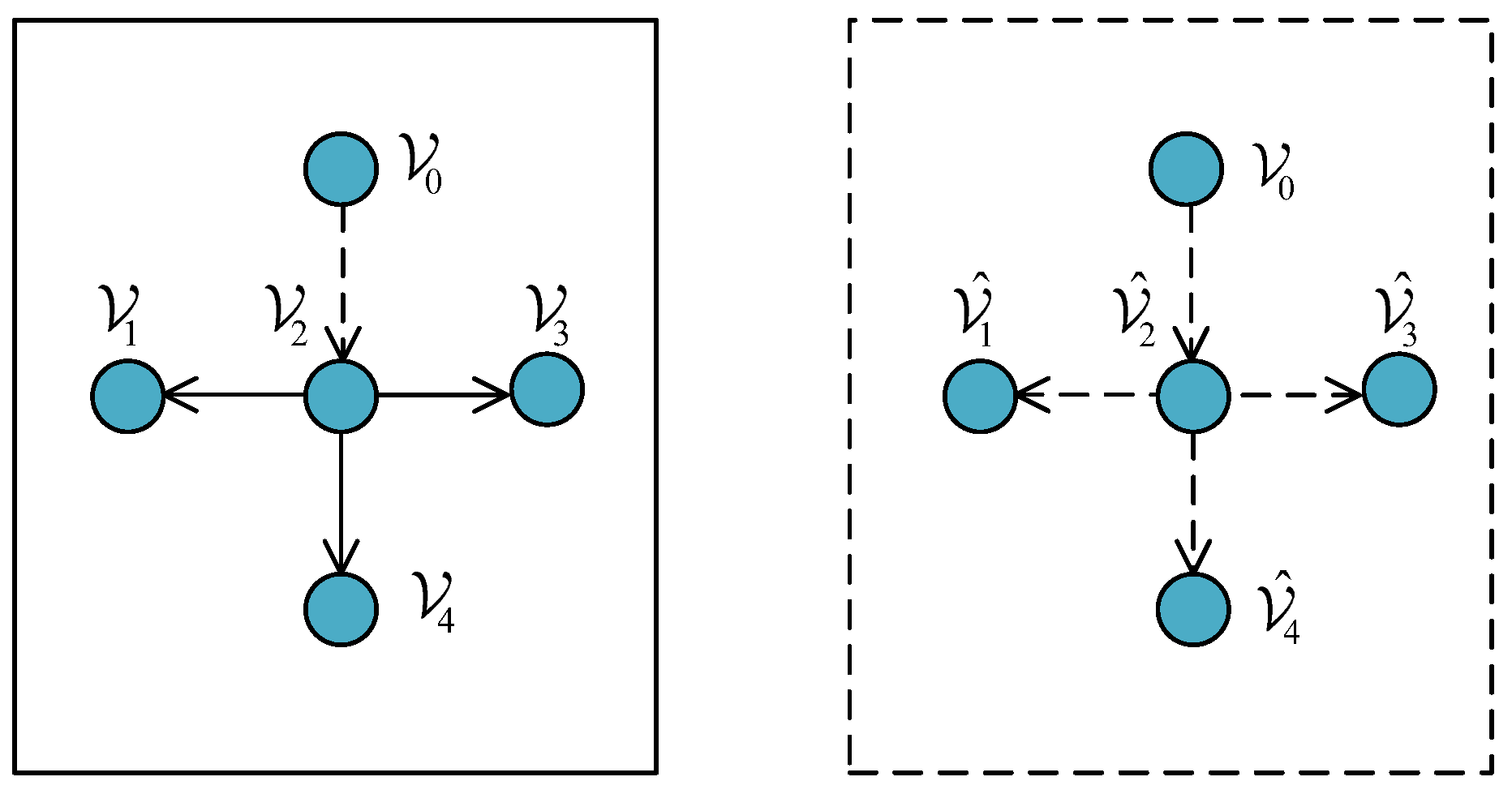
2.2. Problem Statement

Consider a group of N non-holonomic followers moving in a spatiotemporal flowfield and a non-holonomic virtual leader moving without a spatiotemporal flowfield in the fixed inertial reference frame $\mathbb{W}$. The mapping $f_{p_i}\left(t\right)={\left[f_{p_{xi}}\left(t\right),f_{p_{yi}}\left(t\right),f_{p_{zi}}\left(t\right)\right]}^T\in {\mathbb{R}}^3$ is the spatiotemporal flowfield, which is a $C^1$ smooth and bounded function of the position p in the fixed inertial reference frame $\mathbb{W}$ and the time t. Moving in the spatiotemporal flowfield, the non-holonomic dynamics of each follower are given by

$$\left\{\begin{array}{c}{\dot{p}}_i=v_i{x}_i+f_i\left(p_i,t\right)\hfill \\ {\dot{\alpha }}_i={\mathsf{\Omega }}_{{\alpha }_i}\hfill \\ {\dot{\theta }}_i={\mathsf{\Omega }}_{{\theta }_i}\hfill \\ {\dot{v}}_i=u_{v_i}\hfill \\ {\dot{\mathsf{\Omega }}}_{{\alpha }_i}=u_{{\alpha }_i}\hfill \\ {\dot{\mathsf{\Omega }}}_{{\theta }_i}=u_{{\theta }_i},\hfill \end{array}\right.$$

(3)

where ${\alpha }_i\in \mathbb{R}$ and ${\theta }_i\in \mathbb{R}$ denote its pitch angle and yaw angle, respectively. $x_i={\left[cos{\alpha }_{i}cos{\theta }_i,cos{\alpha }_{i}sin{\theta }_i,sin{\alpha }_i\right]}^T\in {\mathbb{R}}^3$ is the unit direction vector of the surge velocity. $v_i\in \mathbb{R}$, ${\mathsf{\Omega }}_{{\alpha }_i}\in \mathbb{R}$ and ${\mathsf{\Omega }}_{{\theta }_i}\in \mathbb{R}$ denote its surge velocity, its pitch angular velocity, and its yaw angular velocity, respectively. $u_{v_i}\in \mathbb{R}$, $u_{{\alpha }_i}\in \mathbb{R}$ and $u_{{\theta }_i}\in \mathbb{R}$ respectively denote its surge acceleration, its pitch acceleration, and its yaw acceleration, which are the designed control inputs. The dynamics of the non-holonomic virtual leader is the same as (3) with replacing the subscript by 0 and removing the spatiotemporal flowfield. In the three-dimensional space, the motion of the virtual leader satisfies the following assumption.

Assumption 3.

The virtual leader moves around its desired orbit on the target sphere.

Let

$$\begin{array}{cc}\hfill v_{f_{li}}& =\sqrt{2v_{f_{li}}\left(f_{li}^T\left(R{y}_{f_{pi}}\right)\right)-{∥f_{li}∥}^2+{\left(v_{li}\right)}^2},\hfill \\ \hfill {\alpha }_{f_{p_i}}& =arctan\frac{v_{i}sin{\alpha }_i+f_{p_{zi}}}{\sqrt{{(v_{i}cos{\alpha }_{i}cos{\theta }_i+f_{p_{xi}})}^2+{(v_{i}cos{\alpha }_{i}sin{\theta }_i+f_{p_{yi}})}^2}},\hfill \\ \hfill {\theta }_{f_{p_i}}& =arctan2\left(\left(v_{i}cos{\alpha }_{i}sin{\theta }_i+f_{p_{yi}}\right),\left(v_{i}cos{\alpha }_{i}cos{\theta }_i+f_{p_{xi}}\right)\right)\hfill \end{array}$$

(4)

be the total surge velocity projected into the lateral plane $e_x{o}_w{e}_y$, the total pitch angle and the total yaw angle, respectively, where $f_{li}={\left[f_{p_{xi}},f_{p_{yi}},0\right]}^T$, $R={[R_x,R_y,R_z]}^T$, $R_x={\left[0,-1,0\right]}^T$, $R_y={\left[1,0,0\right]}^T$, $R_z={\left[0,0,0\right]}^T$, and $v_{li}=v_{i}cos{\alpha }_i$ is the surge velocity projected into the lateral plane $e_x{o}_w{e}_y$. Based on Equation (4), the Frenet–Serret (F–S) frame is established by

$$\begin{array}{cc}\hfill x_{f_{pi}}& ={\left[cos{\alpha }_{f_{pi}}cos{\theta }_{f_{pi}},cos{\alpha }_{f_{pi}}sin{\theta }_{f_{pi}},sin{\alpha }_{f_{pi}}\right]}^T,\hfill \\ \hfill y_{f_{pi}}& ={\left[-sin{\theta }_{f_{pi}},cos{\theta }_{f_{pi}},0\right]}^T,\hfill \\ \hfill z_{f_{pi}}& ={\left[-sin{\alpha }_{f_{pi}}cos{\theta }_{f_{pi}},-sin{\alpha }_{f_{pi}}sin{\theta }_{f_{pi}},cos{\alpha }_{f_{pi}}\right]}^T,\hfill \end{array}$$

(5)

where $x_{f_{pi}}$ denotes the unit direction vector of the total velocity of each UAV, $y_{f_{pi}}$ denotes the unit principal normal vector and is perpendicular to the projection of $x_{f_{pi}}$ onto the lateral plane $e_x{o}_w{e}_y$, and $z_{f_i}$ denotes the unit binormal vector and complies with $z_{f_{pi}}=x_{f_{pi}}\times y_{f_{pi}}$ with a cross-product symbol ×. To overcome the effect of the spatiotemporal flowfield from the established F–S frame (5) and [27], the F–S formulas of each follower is given by

$$\left\{\begin{array}{c}{\dot{p}}_i=\frac{v_{f_{li}}}{x_{f_{p_i}}^T\left(R{y}_{f_{p_i}}\right)}{x}_{f_{p_i}}\hfill \\ {\dot{x}}_{f_{p_i}}=\left(x_{f_{p_i}}^T\left(R{y}_{f_{p_i}}\right)\right)y_{f_{p_i}}\left(k_{{\theta }_{f_{p_i}}}{u}_{v_i}+{\overline{k}}_{{\theta }_{f_{p_i}}}{\mathsf{\Omega }}_{{\alpha }_i}+{\widehat{k}}_{{\theta }_{f_{p_i}}}{\mathsf{\Omega }}_{{\theta }_i}+d_{{\theta }_{f_{p_i}}}\right)\hfill \\ +z_{f_{p_i}}\left(k_{{\alpha }_{f_{p_i}}}{u}_{v_i}+{\overline{k}}_{{\alpha }_{f_{p_i}}}{\mathsf{\Omega }}_{{\alpha }_i}+{\widehat{k}}_{{\alpha }_{f_{p_i}}}{\mathsf{\Omega }}_{{\theta }_i}+d_{{\alpha }_{f_{p_i}}}\right)\hfill \\ {\dot{y}}_{f_{p_i}}=-\left(R{y}_{f_{p_i}}\right)\left(k_{{\theta }_{f_{p_i}}}{u}_{v_i}+{\overline{k}}_{{\theta }_{f_{p_i}}}{\mathsf{\Omega }}_{{\alpha }_i}+{\widehat{k}}_{{\theta }_{f_{p_i}}}{\mathsf{\Omega }}_{{\theta }_i}+d_{{\theta }_{f_{p_i}}}\right)\hfill \\ {\dot{z}}_{f_{p_i}}=\left(z_{f_{p_i}}^T\left(R{y}_{f_{p_i}}\right)\right)y_{f_{p_i}}\left(k_{{\theta }_{f_{p_i}}}{u}_{v_i}+{\overline{k}}_{{\theta }_{f_{p_i}}}{\mathsf{\Omega }}_{{\alpha }_i}+{\widehat{k}}_{{\theta }_{f_{p_i}}}{\mathsf{\Omega }}_{{\theta }_i}+d_{{\theta }_{f_{p_i}}}\right)\hfill \\ -x_{f_{p_i}}\left(k_{{\alpha }_{f_{p_i}}}{u}_{v_i}+{\overline{k}}_{{\alpha }_{f_{p_i}}}{\mathsf{\Omega }}_{{\alpha }_i}+{\widehat{k}}_{{\alpha }_{f_{p_i}}}{\mathsf{\Omega }}_{{\theta }_i}+d_{{\alpha }_{f_{p_i}}}\right)\hfill \\ {\dot{v}}_{f_{li}}=k_{v_{f_{li}}}{u}_{v_i}+{\overline{k}}_{v_{f_{li}}}{\mathsf{\Omega }}_{{\alpha }_i}+{\widehat{k}}_{v_{f_{li}}}{\mathsf{\Omega }}_{{\theta }_i}+d_{v_{f_{li}}}\hfill \end{array}\right.$$

(6)

on the set

$${\mathsf{\Omega }}_{v_{f_{li}}}=\{v_{f_{li}}\in \mathbb{R}\mid v_{f_{li}}\left(t\right)>2f_M\}$$

(7)

with $f_M$ being the maximum magnitude of $f_{li}$, where

$$\begin{array}{cc}\hfill & k_{{\theta }_{f_{p_i}}}=\frac{-f_{p_i}^T{y}_{f_{p_i}}}{v_i{v}_{f_{li}}},{\overline{k}}_{{\theta }_{f_{p_i}}}=\frac{\left(f_{p_i}^T{y}_{f_{p_i}}\right)tan{\alpha }_i}{v_{f_{li}}},{\widehat{k}}_{{\theta }_{f_{p_i}}}=1-\frac{f_{p_i}^T\left(R{y}_{f_{p_i}}\right)}{v_{f_{li}}},d_{{\theta }_{f_{p_i}}}=\frac{{\dot{f}}_{pi}^T{y}_{f_{p_i}}}{v_{f_{li}}},\hfill \\ \hfill & k_{{\alpha }_{f_{p_i}}}=-\frac{\left(f_{p_i}^T{z}_{f_{p_i}}\right)\left(x_{f_{p_i}}^T\left(R{y}_{f_{p_i}}\right)\right)}{v_i{v}_{f_{li}}},\hfill \\ \hfill & {\overline{k}}_{{\alpha }_{f_{p_i}}}=\frac{v_{li}{\left(x_{f_{p_i}}^T\left(R{y}_{f_{p_i}}\right)\right)}^2}{v_{f_{li}}}-tan{\alpha }_i\left(z_{f_{p_i}}^T\left(R{y}_{f_{p_i}}\right)\right)\frac{\left(x_{f_{p_i}}^T\left(R{y}_{f_{p_i}}\right)\right)\left(v_{f_{li}}-f_{p_i}^T\left(R{y}_{f_{p_i}}\right)\right)}{v_{f_{li}}},\hfill \\ \hfill & {\widehat{k}}_{{\alpha }_{f_{p_i}}}=\frac{z_{f_{p_i}}^T\left(R{y}_{f_{p_i}}\right)\left(x_{f_{p_i}}^T\left(R{y}_{f_{p_i}}\right)\right)\left(f_{p_i}^T{y}_{f_{p_i}}\right)}{v_{f_{li}}},d_{{\alpha }_{f_{p_i}}}=\frac{\left({\dot{f}}_{pi}^T{z}_{f_{p_i}}\right)\left(x_{f_{p_i}}^T\left(R{y}_{f_{p_i}}\right)\right)}{v_{f_{li}}},\hfill \\ \hfill & k_{v_{f_{li}}}=\frac{v_i{cos}^2{\alpha }_i}{\sqrt{v_{li}^2-{∥f_{li}∥}^2+{\left(f_{li}^T\left(R{y}_{f_{p_i}}\right)\right)}^2}}+k_{{\theta }_{f_{p_i}}}\left(f_{li}^T{y}_{f_{p_i}}+\frac{\left(f_{li}^T{y}_{f_{p_i}}\right)\left(f_{li}^T\left(R{y}_{f_{p_i}}\right)\right)}{\sqrt{v_{li}^2-{∥f_{li}∥}^2+{\left(f_{li}^T\left(R{y}_{f_{p_i}}\right)\right)}^2}}\right),\hfill \\ \hfill & {\overline{k}}_{v_{f_{li}}}=\frac{-v_i^{2}cos{\alpha }_{i}sin{\alpha }_i}{\sqrt{v_{li}^2-{∥f_{li}∥}^2+{\left(f_{li}^T\left(R{y}_{f_{p_i}}\right)\right)}^2}}+{\overline{k}}_{{\theta }_{f_{p_i}}}\left(f_{li}^T{y}_{f_{p_i}}+\frac{\left(f_{li}^T{y}_{f_{p_i}}\right)\left(f_{li}^T\left(R{y}_{f_{p_i}}\right)\right)}{\sqrt{v_{li}^2-{∥f_{li}∥}^2+{\left(f_{li}^T\left(R{y}_{f_{p_i}}\right)\right)}^2}}\right),\hfill \end{array}$$

$$\begin{array}{cc}\hfill & {\widehat{k}}_{v_{f_{li}}}={\widehat{k}}_{{\theta }_{f_{p_i}}}\left(f_{li}^T{y}_{f_{p_i}}+\frac{\left(f_{li}^T{y}_{f_{p_i}}\right)\left(f_{li}^T\left(R{y}_{f_{p_i}}\right)\right)}{\sqrt{v_{li}^2-{∥f_{li}∥}^2+{\left(f_{li}^T\left(R{y}_{f_{p_i}}\right)\right)}^2}}\right),\hfill \\ \hfill & d_{v_{f_{li}}}=d_{{\theta }_{f_{p_i}}}\left(f_{li}^T{y}_{f_{p_i}}+\frac{\left(f_{li}^T{y}_{f_{p_i}}\right)\left(f_{li}^T\left(R{y}_{f_{p_i}}\right)\right)}{\sqrt{v_{li}^2-{∥f_{li}∥}^2+{\left(f_{li}^T\left(R{y}_{f_{p_i}}\right)\right)}^2}}\right)+{\dot{f}}_{p_i}^T\left(R{y}_{f_{p_i}}\right)\hfill \\ \hfill & +\left(f_{li}^T\left(R{y}_{f_{p_i}}\right)\right)\left({\dot{f}}_{p_i}^T\left(R{y}_{f_{p_i}}\right)\right)-\frac{f_{li}^T{\dot{f}}_{p_i}}{\sqrt{v_{li}^2-{∥f_{li}∥}^2+{\left(f_{li}^T\left(R{y}_{f_{p_i}}\right)\right)}^2}}.\hfill \end{array}$$

From the definition of the spherical function (1), sphere tracking is achieved if

$$\left|\underset{t\to \infty }{lim}{\lambda }_i\left(p_i\left(t\right)\right)\right|\le {\varpi }_1.$$

(8)

with a sufficiently small positive constant ${\varpi }_1$.

Note that the desired orbit $C_i^{\ast }$ whose center is on the $e_z$ has the same desired polar angle ${\varphi }_i^{\ast }\in (-\pi /2,\pi /2)$, and the others can be translated into this case by the coordinate system rotation. Define

$${\varphi }_i\left(t\right)=arctan\frac{p_{zi}}{∥p_{li}∥}$$

(9)

with $p_{li}={\left[p_{xi},p_{yi},0\right]}^T$. Let

$$e_{{\varphi }_i}={\varphi }_i-{\varphi }_i^{\ast }$$

(10)

be the errors of orbit tracking. Orbit tracking is achieved if

$$\left|\underset{t\to \infty }{lim}{e}_{{\varphi }_i}\left(t\right)\right|\le {\varpi }_2$$

(11)

with a sufficiently small positive constant ${\varpi }_2$.

Note that ${\alpha }_{f_{p_i}}\left(t\right)$ and

$${\delta }_{f_{p_i}}\left(t\right)=arctan2\left(-E_i^T{y}_{f_{p_i}},E_i^{T}R{y}_{f_{p_i}}\right)$$

(12)

are the angle tracking errors between the movement direction of UAV i and the tangential vector of the orbit, where $E_i={\left[sin{\psi }_i,-cos{\psi }_i,0\right]}^T$. Orbital angle tracking is achieved if

$$\begin{array}{cc}\hfill \left|\underset{t\to \infty }{lim}{\alpha }_{f_{p_i}}\left(t\right)\right|& \le {\varpi }_3,\hfill \end{array}$$

(13)

$$\begin{array}{cc}\hfill \left|\underset{t\to \infty }{lim}{\delta }_{f_{p_i}}\left(t\right)\right|& \le {\varpi }_4,\hfill \end{array}$$

(14)

with sufficiently small positive constants ${\varpi }_3$ and ${\varpi }_4$.

Define the azimuthal angle by

$${\psi }_i\left(t\right)={\int }_{t_0}^t-\frac{1}{∥p_{li}\left(s\right)∥}{v}_{f_{li}}\left(s\right)cos{\delta }_{f_{li}}\left(s\right)ds.$$

(15)

on the set

$${\mathsf{\Omega }}_{{\varphi }_i}=\{p_i\in {\mathbb{R}}^3\mid p_{x_i}^2\left(t\right)+p_{y_i}^2\left(t\right)>0\}.$$

(16)

The formation is achieved if

$$\left|\underset{t\to \infty }{lim}\left({\psi }_i\left(t\right)-{\psi }_j\left(t\right)-\left({\psi }_i^{\ast }-{\psi }_j^{\ast }\right)\right)\right|\le {\varpi }_5,j\in {\mathcal{N}}_i,$$

(17)

where ${\varpi }_5$ is a sufficiently small positive constant and ${\psi }^{\ast }={\left[{\psi }_1^{\ast },{\psi }_2^{\ast },\cdots ,{\psi }_n^{\ast }\right]}^T$ is the time-invariant formation pattern.

Remark 2.

In this paper, the spherical formation tracking system considers the non-holonomic constraint in (6), the position constraints in (2) and (16), the velocity constraint in (7), and the time-varying delays satisfying Assumption 2 in the directed communication network, which makes the control problem more complex.

Without consideration of time delays, the formation tracking control in [27] for multiple UAVs uses the relative azimuthal angle instead of the absolute azimuthal angle by using the symmetric property of the Laplacian matrix of the bidirectional graph due to the formation subsystem coupling with the tracking subsystems. The asymmetric property of the Laplacian matrix of directed graph and time delays make the design different and more difficult. Hence, a virtual-structure-like system is given to form the formation with time delays in this paper. As an example illustrated in Figure 1, the communication topology among four followers and a virtual leader is on the left, and the communication topology for the virtual-structure-like system is on the right, where the ith node ${\widehat{\mathcal{V}}}_i$ in the virtual-structure-like system is a reference associated with the ith follower ${\mathcal{V}}_i$, the node ${\widehat{\mathcal{V}}}_0$ in the virtual-structure-like system corresponds to the virtual leader ${\mathcal{V}}_0$, and the edges of the virtual-structure-like system are the same as the edges among all followers and the virtual leader.

Under Assumption 3, the surge, pitch, and yaw accelerations for the virtual leader ${\mathcal{V}}_0$ are provided such that

$$\begin{array}{cc}\hfill u_{v_0}& ={\dot{v}}_0^{\ast },\hfill \\ \hfill u_{{\alpha }_0}& =0,\hfill \\ \hfill u_{{\theta }_0}& =\frac{u_{v_0}}{\rho cos{\varphi }_0^{\ast }},\hfill \end{array}$$

(18)

where $v_0^{\ast }\left(t\right)$ is a smooth and bounded signal and $v_0\left(0\right)=v_0^{\ast }\left(0\right)$, ${\lambda }_0\left(0\right)=0$, ${\varphi }_0\left(0\right)={\varphi }_0^{\ast }$, ${\alpha }_0\left(0\right)=0$ and ${\delta }_0\left(0\right)=0$. Due to the time delays in the directed communication network, the virtual-structure-like system ${\psi }_{ri}$ associated with formation is introduced by

$${\dot{\psi }}_{ri}=-\frac{v_{ri}}{∥p_{li}∥},$$

(19)

with

$$\begin{array}{cc}\hfill v_{ri}=& -∥p_{li}∥\left(f(({\psi }_{ri}-{\psi }_i^{\ast }),t)-k\left(\sum _{j=1}^n{a}_{ij}\left({\psi }_{ri}(t-\tau \left(t\right))-{\psi }_i^{\ast }-{\psi }_{rj}(t-\tau \left(t\right))+{\psi }_j^{\ast }\right)\right.\right.\hfill \\ \hfill & \left.\left.+b_i\left({\psi }_{ri}\left(t\right)-{\psi }_i^{\ast }-{\psi }_0\left(t\right)\right)\right)\right),\hfill \end{array}$$

(20)

where k is the azimuthal angle damping gain and is a positive constant, ${\psi }_0$ is the azimuthal angle of the virtual leader, $f(({\psi }_{ri}-{\psi }_i^{\ast }),t)$ is a positive function which satisfies that $\left|f(({\psi }_{ri}-{\psi }_i^{\ast }),t)-f({\psi }_0,t)\right|\le \chi \left|{\psi }_{ri}-{\psi }_i^{\ast }-{\psi }_0\right|$ and $f(({\psi }_{ri}-{\psi }_i^{\ast }),t)<-\frac{2f_M}{∥p_{li}∥}+k\left({\displaystyle \sum _{j=1}^n}{a}_{ij}\left(-2\pi -{\psi }_i^{\ast }+{\psi }_j^{\ast }\right)+b_i\left(-2\pi -{\psi }_i^{\ast }\right)\right)$ with $\chi$ being a positive constant and $f({\psi }_0,t)$ denoting the azimuthal angular velocity of virtual leader such that

$${\dot{\psi }}_0=f({\psi }_0,t).$$

(21)

Let

$$e_{{\psi }_{ri}}={\psi }_{ri}-{\psi }_i^{\ast }-{\psi }_0$$

(22)

be the virtual-structure-like system error. Differentiating (22) along (19) and (21) yields

$${\dot{e}}_{{\psi }_r}=-kB{e}_{{\psi }_r}\left(t\right)-kL{e}_{{\psi }_r}(t-\tau \left(t\right))+F.$$

(23)

where $e_{{\psi }_r}={\left[e_{{\psi }_{r1}},e_{{\psi }_{r2}},\cdots ,e_{{\psi }_{rn}}\right]}^T$, and $F={\left[F_1,F_2,\cdots ,F_n\right]}^T$ with $F_i=f(({\psi }_{ri}-{\psi }_i^{\ast }),t)-f({\psi }_0,t)$. By using Theorem 1 in [33], the resulting system (23) is asymptotically stable. As a result, the formation objective turns to the virtual-structure-like system tracking objective such that

$$\left|\underset{t\to \infty }{lim}\left({\psi }_i\left(t\right)-{\psi }_{ri}\left(t\right)\right)\right|\le {\varpi }_6,$$

(24)

where ${\varpi }_6$ is a sufficiently small positive constant.

Remark 3.

The stability of the resulting system (23) is proved by the following Lyapunov–Krasovskii functional

$$V\left(t\right)=e_{{\psi }_r}^T\left(t\right)P{e}_{{\psi }_r}\left(t\right)+{\int }_{t-\tau \left(t\right)}^t{e}_{{\psi }_r}^T\left(s\right)Q{e}_{{\psi }_r}\left(s\right)ds+{\int }_{-\tau \left(t\right)}^0{\int }_{t+\beta }^t{\dot{e}}_{{\psi }_r}^T\left(s\right)R{\dot{e}}_{{\psi }_r}\left(s\right)dsd\beta ,$$

(25)

where P, Q, and R are positive definite matrices. The details can be found in [33].

Remark 4.

Without the proposed virtual-structure-like system, it fails to deal with the issue of state constraints and time delays in the directed communication network by directly using the Lyapunov method. Based on the virtual-structure-like system, the delayed formation tracking problem with state constraints is translated into the tracking problem with state constraints.

To satisfy the position and velocity constraints, a barrier function is introduced and defined as follows:

Definition 1.

For $a_i,b_i\in \mathcal{R}$, a barrier function $h_x\left(x_i\right)$, defined on an open set $(a_i,b_i)$ containing the desired point ${\mathcal{D}}_{x_i}$, is semi-positive definite, convex, and $C^2$ continuous at every point of $(a_i,b_i)$, has the following properties:

(C1)

${lim}_{x_i\to a_i}{h}_x\left(x_i\right)=+\infty$ and ${lim}_{x_i\to a_i}\nabla h_x\left(x_i\right)=-\infty$,

(C2)

${lim}_{x_i\to b_i}{h}_x\left(x_i\right)=+\infty$ and ${lim}_{x_i\to b_i}\nabla h_x\left(x_i\right)=+\infty$,

(C3)

$\nabla h_x\left({\mathcal{D}}_{x_i}\right)=0$.

The definition of spherical formation tracking control problem with state constraints and time delays is given as follows.

Spherical formation tracking problem with state constraints and time delays. Suppose that Assumptions 1, 2, and 3 hold. Consider the system (3) with the initial position of each follower $p_i\left(0\right)\in {\mathsf{\Omega }}_{{\lambda }_i}\cap {\mathsf{\Omega }}_{{\varphi }_i}$ and the initial velocity of each follower $v_{li}\left(0\right)>f_{M_1}$. Designing a spherical formation tracking control law for each follower such that the control objectives (8), (11), (13), (14), and (24) are achieved with position constraints (2) (16) and velocity constraint (7).

Remark 5.

This paper achieves the velocity constraints (7) by limiting the initial velocity $v_{li}\left(0\right)>f_{M_1}$ instead of $v_{f_{li}}\left(0\right)>2f_M$. From the first equation of (4), the equation becomes

$$\begin{array}{cc}\hfill {\left(v_{li}\right)}^2& =v_{f_{li}}^2-2v_{f_{li}}\left(f_{li}^T\left(R{y}_{f_{pi}}\right)\right)+{∥f_{li}∥}^2,\hfill \\ \hfill & ={\left(v_{f_{li}}-∥f_{li}^T\left(R{y}_{f_{pi}}\right)∥\right)}^2-{∥f_{li}^T\left(R{y}_{f_{pi}}\right)∥}^2+{∥f_{li}∥}^2.\hfill \end{array}$$

(26)

According to (26) when $t=0$, Equation

$$v_{li}\left(0\right)>f_{M_1}$$

(27)

yields

$$v_{f_{li}}\left(0\right)>2f_M.$$

(28)

In practice, $f_{M_1}$ can be chosen as $\sqrt{5}{f}_M$.

3. Main Results

Let

$$\begin{array}{cc}\hfill N_i& ={\left[-sin{\varphi }_{i}cos{\psi }_i,-sin{\varphi }_{i}sin{\psi }_i,cos{\varphi }_i\right]}^T,\hfill \\ \hfill E_i& ={\left[sin{\psi }_i,-cos{\psi }_i,0\right]}^T,\hfill \\ \hfill D_i& ={\left[-cos{\varphi }_{i}cos{\psi }_i,-cos{\varphi }_{i}sin{\psi }_i,-sin{\varphi }_i\right]}^T,\hfill \end{array}$$

(29)

be the north east down (NED) coordinate system. Differentiating (1) along the system (6), the dynamics of ${\lambda }_i$ associated with sphere tracking are

$${\dot{\lambda }}_i=\frac{1}{{\rho }_i}\frac{v_{f_{li}}}{x_{f_{p_i}}^T\left(R{y}_{f_{p_i}}\right)}{D}_i^T{x}_{f_{p_i}}=-\frac{1}{{\rho }_i}{v}_{f_{li}}(cos{\varphi }_{i}sin{\delta }_{f_{p_i}}+sin{\varphi }_{i}tan{\alpha }_{f_{p_i}}).$$

(30)

Differentiating (10) along the system (6), the dynamics of $e_{{\varphi }_i}$ associated with orbit tracking are

$${\dot{e}}_{{\varphi }_i}=\frac{1}{∥p_i∥}\frac{v_{f_{li}}}{x_{f_{p_i}}^T\left(R{y}_{f_{p_i}}\right)}{N}_i^T{x}_{f_{p_i}}=-\frac{1}{∥p_i∥}{v}_{f_{li}}(sin{\varphi }_{i}sin{\delta }_{f_{p_i}}-cos{\varphi }_{i}tan{\alpha }_{f_{p_i}}).$$

(31)

From the system (6), the dynamics of the angle error ${\alpha }_{f_{p_i}}$ are

$${\dot{\alpha }}_{f_{p_i}}=k_{{\alpha }_{f_{p_i}}}{u}_{v_i}+{\overline{k}}_{{\alpha }_{f_{p_i}}}{\mathsf{\Omega }}_{{\alpha }_i}+{\widehat{k}}_{{\alpha }_{f_{p_i}}}{\mathsf{\Omega }}_{{\theta }_i}+d_{{\alpha }_{f_{p_i}}}.$$

(32)

Differentiating (12) along the system (6), the dynamics of the angle error ${\delta }_{f_{p_i}}$ are

$${\dot{\delta }}_{f_{p_i}}=\frac{1}{∥p_{li}∥}{v}_{f_{li}}cos{\delta }_{f_{p_i}}+k_{{\theta }_{f_{p_i}}}{u}_{v_i}+{\overline{k}}_{{\theta }_{f_{p_i}}}{\mathsf{\Omega }}_{{\alpha }_i}+{\widehat{k}}_{{\theta }_{f_{p_i}}}{\mathsf{\Omega }}_{{\theta }_i}+d_{{\theta }_{f_{p_i}}}.$$

(33)

Based on the virtual-structure-like system, the virtual-structure-like system tracking error is defined by

$$e_{{\psi }_i}={\psi }_i-{\psi }_{ri}.$$

(34)

Differentiating (34) along the system (6) and (19), the dynamics of (34) are given by

$${\dot{e}}_{{\psi }_i}=-\frac{1}{∥p_{li}∥}\frac{v_{f_{li}}}{x_{f_{p_i}}^T\left(R{y}_{f_{p_i}}\right)}{E}_i^T{x}_{f_{p_i}}+\frac{v_{ri}}{∥p_{li}∥}=\frac{1}{∥p_{li}∥}{v}_{f_{li}}(1-cos{\delta }_{f_{p_i}})-e_{v_{{\psi }_i}},$$

(35)

where $e_{v_{{\psi }_i}}=v_{{\psi }_i}-{\dot{\psi }}_{ri}$ with $v_{{\psi }_i}=\frac{v_{f_{li}}}{∥p_{li}∥}$.

From the above discussion, the open-loop equations for the spherical formation tracking control system with state constraints and time delays are given by (30), (31), (32), (33), and (35).

Controller Design

The dynamic surface method is applied to this design process. Two steps are included in the process of the dynamic surface method. The pitch and yaw angular velocities $\{{\mathsf{\Omega }}_{{\alpha }_i},{\mathsf{\Omega }}_{{\theta }_i}\}$ for each UAV are regarded as the virtual controls $\{{\overline{\mathsf{\Omega }}}_{{\alpha }_i},{\overline{\mathsf{\Omega }}}_{{\theta }_i}\}$. Step 1 obtains the surge acceleration $u_{v_i}$, the virtual pitch angular velocity ${\overline{\mathsf{\Omega }}}_{{\alpha }_i}$, and the virtual yaw angular velocity ${\overline{\mathsf{\Omega }}}_{{\theta }_i}$ by solving the designed equations: $k_{{\alpha }_{f_{p_i}}}{u}_{v_i}+{\overline{k}}_{{\alpha }_{f_{p_i}}}{\overline{\mathsf{\Omega }}}_{{\alpha }_i}+{\widehat{k}}_{{\alpha }_{f_{p_i}}}{\overline{\mathsf{\Omega }}}_{{\theta }_i}$, $k_{{\theta }_{f_{p_i}}}{u}_{v_i}+{\overline{k}}_{{\theta }_{f_{p_i}}}{\overline{\mathsf{\Omega }}}_{{\alpha }_i}+{\widehat{k}}_{{\theta }_{f_{p_i}}}{\overline{\mathsf{\Omega }}}_{{\theta }_i}$ and $k_{v_{f_{li}}}{u}_{v_i}+{\overline{k}}_{v_{f_{li}}}{\overline{\mathsf{\Omega }}}_{{\alpha }_i}+{\widehat{k}}_{v_{f_{li}}}{\overline{\mathsf{\Omega }}}_{{\theta }_i}$. The pitch and yaw accelerations $\{u_{{\alpha }_i},u_{{\theta }_i}\}$ are designed by means of the first-order filters in step 2.

Step 1. Consider the open-loop spherical formation tracking control system composed of (30), (31), (32), (33), and (35), and the barrier Lyapunov function is

$$\begin{array}{cc}\hfill V_I=& \sum _{i=1}^n\left(h_{\lambda }\left({\lambda }_i\right)+h_{\varphi }\left({\varphi }_i\right)-ln\left(cos{\alpha }_{f_{p_i}}\right)-ln\left({cos}^2\frac{{\delta }_{f_{p_i}}}{2}\right)\right)+\frac{1}{2}\sum _{i=1}^n{e}_{{\psi }_i}^2\hfill \\ \hfill & +\sum _{i=1}^n\left(ln\left(\frac{v_{f_{li}}-2f_M}{v_{ri}-2f_M}\right)+\frac{v_{ri}-2f_M}{v_{f_{li}}-2f_M}-1\right),\hfill \end{array}$$

(36)

where $h_{\lambda }\left({\lambda }_i\right)$ when $x=\lambda$, $a_i=-{\epsilon }_i$, $b_i={\epsilon }_i$ and ${\mathcal{D}}_{{\lambda }_i}=0$, and $h_{\varphi }\left({\varphi }_i\right)$ when $x=\varphi$, $a_i=-\frac{\pi }{2}$, $b_i=\frac{\pi }{2}$ and ${\mathcal{D}}_{{\varphi }_i}={\varphi }_i^{\ast }$, are barrier functions satisfying Definition 1. The detailed forms of the barrier functions can be found in [27]. These barrier functions contribute to the objectives of sphere tracking (8) and orbit tracking (11) with position constraints (2) and (16). In (36), the third and fourth terms contribute to yielding the objective of orbital angles tracking (13) and (14), respectively. The fifth term contributes to the objective of the virtual-structure-like system tracking (24). The last term is the barrier function satisfying Definition 1, which is used to guarantee the velocity constraint (7).

Differentiating (36) along the open-loop spherical formation tracking control system yields

$$\begin{array}{cc}\hfill {\dot{V}}_I=& \sum _{i=1}^{n}tan{\alpha }_{f_{p_i}}\left({\overline{\Delta }}_{{\alpha }_{f_{p_i}}}+{\Delta }_{{\alpha }_{f_{p_i}}}\right)+\sum _{i=1}^{n}tan\frac{{\delta }_{f_{p_i}}}{2}\left({\overline{\Delta }}_{{\theta }_{f_{p_i}}}+{\Delta }_{{\theta }_{f_{p_i}}}\right)\hfill \\ \hfill & +\sum _{i=1}^n{e}_{v_{{\psi }_i}}\left(\frac{∥p_{li}∥}{{\left(v_{f_{li}}-2f_M\right)}^2}{\overline{\Delta }}_{v_{f_{li}}}+{\Delta }_{v_{f_{li}}}\right),\hfill \end{array}$$

(37)

where

$$\begin{array}{cc}\hfill {\Delta }_{{\alpha }_{f_{p_i}}}=& -\frac{1}{{\rho }_i}\nabla h_{\lambda }\left({\lambda }_i\right)v_{f_{li}}sin{\varphi }_i+\frac{1}{∥p_i∥}\nabla h_e\left({\varphi }_i\right)v_{f_{li}}cos{\varphi }_i+d_{{\alpha }_{f_{p_i}}},\hfill \\ \hfill {\Delta }_{{\theta }_{f_{p_i}}}=& -2\frac{1}{{\rho }_i}\nabla h_{\lambda }\left({\lambda }_i\right)v_{f_{li}}cos{\varphi }_i{cos}^2\frac{{\delta }_{f_{p_i}}}{2}-2\frac{1}{∥p_i∥}\nabla h_e\left({\varphi }_i\right)v_{f_{li}}sin{\varphi }_i{cos}^2\frac{{\delta }_{f_{p_i}}}{2}\hfill \end{array}$$

$$\begin{array}{cc}\hfill & +\frac{1}{∥p_{li}∥}{v}_{f_{li}}cos{\delta }_{f_{p_i}}+\frac{1}{∥p_{li}∥}{e}_{{\psi }_i}{v}_{f_{li}}sin{\delta }_{f_{p_i}}+d_{{\theta }_{f_{p_i}}},\hfill \\ \hfill {\Delta }_{v_{f_{li}}}=& \frac{∥p_{li}∥}{(v_{ri}-2f_M)(v_{f_{li}}-2f_M)}\left(\frac{\partial v_{ri}}{\partial p_{xi}}\left(v_{i}cos{\alpha }_{i}cos{\theta }_i+f_{xi}\right)+\frac{\partial v_{ri}}{\partial p_{yi}}\left(v_{i}cos{\alpha }_{i}sin{\theta }_i\right.\right.\hfill \\ \hfill & \left.\left.+f_{yi}\right)+\frac{\partial v_{ri}}{\partial p_{zi}}\left(v_{i}sin{\alpha }_i+f_{zi}\right)+\frac{\partial v_{ri}}{\partial t}\right)-e_{{\psi }_i}+\frac{∥p_{li}∥}{{(v_{f_{li}}-2f_M)}^2}{d}_{v_{f_{li}}}.\hfill \end{array}$$

Designing

$$\begin{array}{cc}\hfill {\overline{\Delta }}_{{\alpha }_{f_{p_i}}}& =k_{{\alpha }_{f_{p_i}}}{u}_{v_i}+{\overline{k}}_{{\alpha }_{f_{p_i}}}{\overline{\mathsf{\Omega }}}_{{\alpha }_i}+{\widehat{k}}_{{\alpha }_{f_{p_i}}}{\overline{\mathsf{\Omega }}}_{{\theta }_i}=-{\Delta }_{{\alpha }_{f_{p_i}}}-c_{1}sin{\alpha }_{f_{p_i}},\hfill \\ \hfill {\overline{\Delta }}_{{\theta }_{f_{p_i}}}& =k_{{\theta }_{f_{p_i}}}{u}_{v_i}+{\overline{k}}_{{\theta }_{f_{p_i}}}{\overline{\mathsf{\Omega }}}_{{\alpha }_i}+{\widehat{k}}_{{\theta }_{f_{p_i}}}{\overline{\mathsf{\Omega }}}_{{\theta }_i}=-{\Delta }_{{\theta }_{f_{p_i}}}-c_{2}sin\frac{{\delta }_{f_{p_i}}}{2},\hfill \\ \hfill {\overline{\Delta }}_{v_{f_{li}}}& =k_{v_{f_{li}}}{u}_{v_i}+{\overline{k}}_{v_{f_{li}}}{\overline{\mathsf{\Omega }}}_{{\alpha }_i}+{\widehat{k}}_{v_{f_{li}}}{\overline{\mathsf{\Omega }}}_{{\theta }_i}=-\frac{{(v_{f_{li}}-2f_M)}^2}{∥p_{li}∥}\left({\Delta }_{v_{f_{li}}}+c_3{e}_{v_{{\psi }_i}}\right)\hfill \end{array}$$

(38)

where $c_1$, $c_2$, and $c_3$ are the positive constants. Noting that

$$\begin{array}{cc}\hfill g_{k_i}& =\left|\begin{array}{ccc}{k}_{{\alpha }_{f_{p_i}}}& {\overline{k}}_{{\alpha }_{f_{p_i}}}& {\widehat{k}}_{{\alpha }_{f_{p_i}}}\\ k_{{\theta }_{f_{p_i}}}& {\overline{k}}_{{\theta }_{f_{p_i}}}& {\widehat{k}}_{{\theta }_{f_{p_i}}}\\ k_{v_{f_{li}}}& {\overline{k}}_{v_{f_{li}}}& {\widehat{k}}_{v_{f_{li}}}\end{array}\right|=\frac{v_i{v}_{li}{cos}^2{\alpha }_{f_{p_i}}}{{\left(v_{f_{li}}\right)}^2}\ne 0\hfill \end{array}$$

under the condition that $v_{f_{li}}>2f_M$, we have

$$\begin{array}{cc}\hfill u_{v_i}=& g_{k_i}^{-1}\left({\overline{\Delta }}_{{\theta }_{f_{p_i}}}\left({\overline{k}}_{{\alpha }_{f_{p_i}}}{\widehat{k}}_{v_{f_{li}}}-{\overline{k}}_{v_{f_{li}}}{\widehat{k}}_{{\alpha }_{f_{p_i}}}\right)-{\overline{\Delta }}_{{\alpha }_{f_{p_i}}}\left({\overline{k}}_{{\theta }_{f_{p_i}}}{\widehat{k}}_{v_{f_{li}}}-{\widehat{k}}_{{\theta }_{f_{p_i}}}{\overline{k}}_{v_{f_{li}}}\right)\right.\hfill \\ \hfill & \left.+{\overline{\Delta }}_{v_{f_{li}}}\left({\widehat{k}}_{{\theta }_{f_{p_i}}}{\overline{k}}_{{\alpha }_{f_{p_i}}}-{\widehat{k}}_{{\alpha }_{f_{p_i}}}{\overline{k}}_{{\theta }_{f_{p_i}}}\right)\right),\hfill \\ \hfill {\overline{\mathsf{\Omega }}}_{{\alpha }_i}=& g_{k_i}^{-1}\left(-{\overline{\Delta }}_{{\theta }_{f_{p_i}}}\left(k_{{\alpha }_{f_{p_i}}}{\widehat{k}}_{v_{f_{li}}}-{\widehat{k}}_{{\alpha }_{f_{p_i}}}{k}_{v_{f_{li}}}\right)+{\overline{\Delta }}_{{\alpha }_{f_{p_i}}}\left(k_{{\theta }_{f_{p_i}}}{\widehat{k}}_{v_{f_{li}}}-{\widehat{k}}_{{\theta }_{f_{p_i}}}{k}_{v_{f_{li}}}\right)\right.\hfill \\ \hfill & \left.-{\overline{\Delta }}_{v_{f_{li}}}\left({\widehat{k}}_{{\theta }_{f_{p_i}}}{k}_{{\alpha }_{f_{p_i}}}^{u_{v_i}}-k_{{\theta }_{f_{p_i}}}{\widehat{k}}_{{\alpha }_{f_{p_i}}}\right)\right),\hfill \\ \hfill {\overline{\mathsf{\Omega }}}_{{\theta }_i}=& g_{k_i}^{-1}\left({\overline{\Delta }}_{{\theta }_{f_{p_i}}}\left(k_{{\alpha }_{f_{p_i}}}{\overline{k}}_{v_{f_{li}}}-{\overline{k}}_{{\alpha }_{f_{p_i}}}{k}_{v_{f_{li}}}\right)-{\overline{\Delta }}_{{\alpha }_{f_{p_i}}}\left(k_{{\theta }_{f_{p_i}}}{\overline{k}}_{v_{f_{li}}}-k_{v_{f_{li}}}{\overline{k}}_{{\theta }_{f_{p_i}}}\right)\right.\hfill \\ \hfill & \left.+{\overline{\Delta }}_{v_{f_{li}}}\left({\overline{k}}_{{\theta }_{f_{p_i}}}{k}_{{\alpha }_{f_{p_i}}}-k_{{\theta }_{f_{p_i}}}{\overline{k}}_{{\alpha }_{f_{p_i}}}\right)\right).\hfill \end{array}$$

(39)

Let the first-order filters for ${\overline{\mathsf{\Omega }}}_{{\alpha }_i}$ and ${\overline{\mathsf{\Omega }}}_{{\theta }_i}$ be

$$\begin{array}{cc}\hfill {\tau }_1{\dot{\tilde{\mathsf{\Omega }}}}_{{\alpha }_i}+{\tilde{\mathsf{\Omega }}}_{{\alpha }_i}& ={\overline{\mathsf{\Omega }}}_{{\alpha }_i}-{\tau }_1{\Delta }_{{\mathsf{\Omega }}_{{\alpha }_i}},{\tilde{\mathsf{\Omega }}}_{{\alpha }_i}\left(0\right)={\overline{\mathsf{\Omega }}}_{{\alpha }_i}\left(0\right),\hfill \\ \hfill {\tau }_2{\dot{\tilde{\mathsf{\Omega }}}}_{{\theta }_i}+{\tilde{\mathsf{\Omega }}}_{{\theta }_i}& ={\overline{\mathsf{\Omega }}}_{{\theta }_i}-{\tau }_2{\Delta }_{{\mathsf{\Omega }}_{{\theta }_i}},{\tilde{\mathsf{\Omega }}}_{{\theta }_i}\left(0\right)={\overline{\mathsf{\Omega }}}_{{\theta }_i}\left(0\right),\hfill \end{array}$$

(40)

where

$$\begin{array}{cc}\hfill {\Delta }_{{\mathsf{\Omega }}_{{\alpha }_i}}& ={\overline{k}}_{{\alpha }_{f_{p_i}}}tan{\alpha }_{f_{p_i}}+{\overline{k}}_{{\theta }_{f_{p_i}}}tan\frac{{\delta }_{f_{p_i}}}{2}+{\overline{k}}_{v_{f_{li}}}\frac{∥p_{li}∥e_{v_{{\psi }_i}}}{{(v_{f_{li}}-2f_M)}^2},\hfill \\ \hfill {\Delta }_{{\mathsf{\Omega }}_{{\theta }_i}}& ={\widehat{k}}_{{\alpha }_{f_{p_i}}}tan{\alpha }_{f_{p_i}}+{\widehat{k}}_{{\theta }_{f_{p_i}}}tan\frac{{\delta }_{f_{p_i}}}{2}+{\widehat{k}}_{v_{f_{li}}}\frac{∥p_{li}∥e_{v_{{\psi }_i}}}{{(v_{f_{li}}-2f_M)}^2},\hfill \end{array}$$

and the positive time constants ${\tau }_1$ and ${\tau }_2$ are set later. Let the error variables be

$$\begin{array}{cc}\hfill {\tilde{e}}_{{\mathsf{\Omega }}_{{\alpha }_i}}& ={\mathsf{\Omega }}_{{\alpha }_i}-{\tilde{\mathsf{\Omega }}}_{{\alpha }_i},{\overline{e}}_{{\mathsf{\Omega }}_{{\alpha }_i}}={\tilde{\mathsf{\Omega }}}_{{\alpha }_i}-{\overline{\mathsf{\Omega }}}_{{\alpha }_i},\hfill \\ \hfill {\tilde{e}}_{{\mathsf{\Omega }}_{{\theta }_i}}& ={\mathsf{\Omega }}_{{\theta }_i}-{\tilde{\mathsf{\Omega }}}_{{\theta }_i},{\overline{e}}_{{\mathsf{\Omega }}_{{\theta }_i}}={\tilde{\mathsf{\Omega }}}_{{\theta }_i}-{\overline{\mathsf{\Omega }}}_{{\theta }_i}.\hfill \end{array}$$

(41)

Substituting (39) and (41) into (37) yields

$$\begin{array}{cc}\hfill {\dot{V}}_{II}=& -c_1\sum _{i=1}^n\frac{{sin}^2{\alpha }_{f_{p_i}}}{cos{\alpha }_{f_{p_i}}}-c_2\sum _{i=1}^n\frac{{sin}^2\frac{{\delta }_{f_{p_i}}}{2}}{cos\frac{{\delta }_{f_{p_i}}}{2}}-c_3\sum _{i=1}^n{e}_{v_{{\psi }_i}}^2\hfill \\ \hfill & +\sum _{i=1}^n\left({\tilde{e}}_{{\mathsf{\Omega }}_{{\alpha }_i}}{\Delta }_{{\mathsf{\Omega }}_{{\alpha }_i}}+{\overline{e}}_{{\mathsf{\Omega }}_{{\alpha }_i}}{\Delta }_{{\mathsf{\Omega }}_{{\alpha }_i}}+{\tilde{e}}_{{\mathsf{\Omega }}_{{\theta }_i}}{\Delta }_{{\mathsf{\Omega }}_{{\theta }_i}}+{\overline{e}}_{{\mathsf{\Omega }}_{{\theta }_i}}{\Delta }_{{\mathsf{\Omega }}_{{\theta }_i}}\right),\hfill \end{array}$$

(42)

Along the design in (39), the spherical formation tracking control system for follower i is rewritten as

$$\begin{array}{cc}\hfill {\dot{\lambda }}_i=& -\frac{1}{{\rho }_i}{v}_{f_{li}}(cos{\varphi }_{i}sin{\delta }_{f_{p_i}}+sin{\varphi }_{i}tan{\alpha }_{f_{p_i}}),\hfill \\ \hfill {\dot{e}}_{{\varphi }_i}=& -\frac{1}{∥p_i∥}{v}_{f_{li}}(sin{\varphi }_{i}sin{\delta }_{f_{p_i}}-cos{\varphi }_{i}tan{\alpha }_{f_{p_i}}),\hfill \\ \hfill {\dot{\alpha }}_{f_{p_i}}=& -c_{1}sin{\alpha }_{f_{p_i}}+\frac{1}{{\rho }_i}\nabla h_{\lambda }\left({\lambda }_i\right)v_{f_{li}}sin{\varphi }_i-\frac{1}{∥p_i∥}\nabla h_e\left({\varphi }_i\right)v_{f_{li}}cos{\varphi }_i\hfill \\ \hfill & +{\overline{k}}_{{\alpha }_{f_{p_i}}}\left({\overline{e}}_{{\mathsf{\Omega }}_{{\alpha }_i}}+{\tilde{e}}_{{\mathsf{\Omega }}_{{\alpha }_i}}\right)+{\widehat{k}}_{{\alpha }_{f_{p_i}}}\left({\overline{e}}_{{\mathsf{\Omega }}_{{\theta }_i}}+{\tilde{e}}_{{\mathsf{\Omega }}_{{\theta }_i}}\right),\hfill \\ \hfill {\dot{\delta }}_{f_{p_i}}=& -c_{2}sin\frac{{\delta }_{f_{p_i}}}{2}+2\frac{1}{{\rho }_i}\nabla h_{\lambda }\left({\lambda }_i\right)v_{f_{li}}cos{\varphi }_i{cos}^2\frac{{\delta }_{f_{p_i}}}{2}+2\frac{1}{∥p_i∥}\nabla h_e\left({\varphi }_i\right)v_{f_{li}}sin{\varphi }_i{cos}^2\frac{{\delta }_{f_{p_i}}}{2}\hfill \\ \hfill & -\frac{1}{∥p_{li}∥}{e}_{{\psi }_i}{v}_{f_{li}}sin{\delta }_{f_{p_i}}+{\overline{k}}_{{\theta }_{f_{p_i}}}\left({\overline{e}}_{{\mathsf{\Omega }}_{{\alpha }_i}}+{\tilde{e}}_{{\mathsf{\Omega }}_{{\alpha }_i}}\right)+{\widehat{k}}_{{\theta }_{f_{p_i}}}\left({\overline{e}}_{{\mathsf{\Omega }}_{{\theta }_i}}+{\tilde{e}}_{{\mathsf{\Omega }}_{{\theta }_i}}\right),\hfill \\ \hfill {\dot{v}}_{f_{li}}=& \frac{-c_3{(v_{f_{li}}-2f_M)}^2}{∥p_{li}∥}{e}_{v_{{\psi }_i}}+\frac{{(v_{f_{li}}-2f_M)}^2}{∥p_{li}∥}{e}_{{\psi }_i}+\frac{v_{f_{li}}-2f_M}{v_{ri}-2f_M}\left(\frac{\partial v_{ri}}{\partial p_{xi}}\left(v_{i}cos{\alpha }_{i}cos{\theta }_i\right.\right.\hfill \\ \hfill & \left.\left.+f_{xi}\right)+\frac{\partial v_{ri}}{\partial p_{yi}}\left(v_{i}cos{\alpha }_{i}sin{\theta }_i+f_{yi}\right)+\frac{\partial v_{ri}}{\partial p_{zi}}\left(v_{i}sin{\alpha }_i+f_{zi}\right)+\frac{\partial v_{ri}}{\partial t}\right)\hfill \\ \hfill & +{\overline{k}}_{v_{f_{li}}}\left({\overline{e}}_{{\mathsf{\Omega }}_{{\alpha }_i}}+{\tilde{e}}_{{\mathsf{\Omega }}_{{\alpha }_i}}\right)+{\widehat{k}}_{v_{f_{li}}}\left({\overline{e}}_{{\mathsf{\Omega }}_{{\theta }_i}}+{\tilde{e}}_{{\mathsf{\Omega }}_{{\theta }_i}}\right),\hfill \\ \hfill {\dot{\tilde{e}}}_{{\mathsf{\Omega }}_{{\alpha }_i}}=& u_{{\alpha }_i}-{\dot{\tilde{\mathsf{\Omega }}}}_{{\alpha }_i},\hfill \\ \hfill {\dot{\overline{e}}}_{{\mathsf{\Omega }}_{{\alpha }_i}}=& -\frac{1}{{\tau }_1}{\overline{e}}_{{\mathsf{\Omega }}_{{\alpha }_i}}-{\Delta }_{{\mathsf{\Omega }}_{{\alpha }_i}}-{\dot{\overline{\mathsf{\Omega }}}}_{{\alpha }_i},\hfill \\ \hfill {\dot{\tilde{e}}}_{{\mathsf{\Omega }}_{{\theta }_i}}=& u_{{\theta }_i}-{\dot{\tilde{\mathsf{\Omega }}}}_{{\theta }_i},\hfill \\ \hfill {\dot{\overline{e}}}_{{\mathsf{\Omega }}_{{\theta }_i}}=& -\frac{1}{{\tau }_2}{\overline{e}}_{{\mathsf{\Omega }}_{{\theta }_i}}-{\Delta }_{{\mathsf{\Omega }}_{{\theta }_i}}-{\dot{\overline{\mathsf{\Omega }}}}_{{\theta }_i}.\hfill \end{array}$$

(43)

Step 2. Consider the spherical formation tracking control system (43) and the following barrier Lyapunov function:

$$V_{II}=V_I+\frac{1}{2}\sum _{i=1}^n{\tilde{e}}_{{\mathsf{\Omega }}_{{\alpha }_i}}^2+\frac{1}{2}\sum _{i=1}^n{\overline{e}}_{{\mathsf{\Omega }}_{{\alpha }_i}}^2+\frac{1}{2}\sum _{i=1}^n{\tilde{e}}_{{\mathsf{\Omega }}_{{\theta }_i}}^2+\frac{1}{2}\sum _{i=1}^n{\overline{e}}_{{\mathsf{\Omega }}_{{\theta }_i}}^2,$$

(44)

Taking the derivative of $V_{II}$ yields

$$\begin{array}{cc}\hfill {\dot{V}}_{II}\le & -c_1\sum _{i=1}^n\frac{{sin}^2{\alpha }_{f_{p_i}}}{cos{\alpha }_{f_{p_i}}}-c_2\sum _{i=1}^n\frac{{sin}^2\frac{{\delta }_{f_{p_i}}}{2}}{cos\frac{{\delta }_{f_{p_i}}}{2}}-c_3\sum _{i=1}^n{e}_{v_{{\psi }_i}}^2+\sum _{i=1}^n\left({\tilde{e}}_{{\mathsf{\Omega }}_{{\alpha }_i}}{\Delta }_{{\mathsf{\Omega }}_{{\alpha }_i}}+{\overline{e}}_{{\mathsf{\Omega }}_{{\alpha }_i}}{\Delta }_{{\mathsf{\Omega }}_{{\alpha }_i}}\right.\hfill \\ \hfill & \left.+{\tilde{e}}_{{\mathsf{\Omega }}_{{\theta }_i}}{\Delta }_{{\mathsf{\Omega }}_{{\theta }_i}}+{\overline{e}}_{{\mathsf{\Omega }}_{{\theta }_i}}{\Delta }_{{\mathsf{\Omega }}_{{\theta }_i}}\right)+\sum _{i=1}^n{\tilde{e}}_{{\mathsf{\Omega }}_{{\alpha }_i}}\left(u_{{\alpha }_i}-{\dot{\tilde{\mathsf{\Omega }}}}_{{\alpha }_i}\right)+\sum _{i=1}^n{\overline{e}}_{{\mathsf{\Omega }}_{{\alpha }_i}}\left(-\frac{1}{{\tau }_1}{\overline{e}}_{{\mathsf{\Omega }}_{{\alpha }_i}}-{\Delta }_{{\mathsf{\Omega }}_{{\alpha }_i}}\right.\hfill \\ \hfill & \left.-{\dot{\overline{\mathsf{\Omega }}}}_{{\alpha }_i}\right)+\sum _{i=1}^n{\tilde{e}}_{{\mathsf{\Omega }}_{{\theta }_i}}\left(u_{{\theta }_i}-{\dot{\tilde{\mathsf{\Omega }}}}_{{\theta }_i}\right)+\sum _{i=1}^n{\overline{e}}_{{\mathsf{\Omega }}_{{\theta }_i}}\left(-\frac{1}{{\tau }_2}{\overline{e}}_{{\mathsf{\Omega }}_{{\theta }_i}}-{\Delta }_{{\mathsf{\Omega }}_{{\theta }_i}}-{\dot{\overline{\mathsf{\Omega }}}}_{{\theta }_i}\right),\hfill \end{array}$$

(45)

which suggests that

$$\begin{array}{cc}\hfill u_{{\alpha }_i}& =-c_4{\tilde{e}}_{{\mathsf{\Omega }}_{{\alpha }_i}}-{\Delta }_{{\mathsf{\Omega }}_{{\alpha }_i}}+{\dot{\tilde{\mathsf{\Omega }}}}_{{\alpha }_i},\hfill \\ \hfill u_{{\theta }_i}& =-c_5{\tilde{e}}_{{\mathsf{\Omega }}_{{\theta }_i}}-{\Delta }_{{\mathsf{\Omega }}_{{\theta }_i}}+{\dot{\tilde{\mathsf{\Omega }}}}_{{\theta }_i},\hfill \end{array}$$

(46)

where $c_4$ and $c_5$ are positive constants. Substituting (46) into (45) yields

$$\begin{array}{cc}\hfill {\dot{V}}_{II}\le & -c_1\sum _{i=1}^n\frac{{sin}^2{\alpha }_{f_{p_i}}}{cos{\alpha }_{f_{p_i}}}-c_2\sum _{i=1}^n\frac{{sin}^2\frac{{\delta }_{f_{p_i}}}{2}}{cos\frac{{\delta }_{f_{p_i}}}{2}}-c_3\sum _{i=1}^n{e}_{v_{{\psi }_i}}^2-c_4\sum _{i=1}^n{\tilde{e}}_{{\mathsf{\Omega }}_{{\alpha }_i}}^2-c_5\sum _{i=1}^n{\tilde{e}}_{{\mathsf{\Omega }}_{{\theta }_i}}^2\hfill \\ \hfill & +\sum _{i=1}^n{\overline{e}}_{{\mathsf{\Omega }}_{{\alpha }_i}}\left(-\frac{1}{{\tau }_1}{\overline{e}}_{{\mathsf{\Omega }}_{{\alpha }_i}}-{\dot{\overline{\mathsf{\Omega }}}}_{{\alpha }_i}\right)+\sum _{i=1}^n{\overline{e}}_{{\mathsf{\Omega }}_{{\theta }_i}}\left(-\frac{1}{{\tau }_2}{\overline{e}}_{{\mathsf{\Omega }}_{{\theta }_i}}-{\dot{\overline{\mathsf{\Omega }}}}_{{\theta }_i}\right).\hfill \end{array}$$

(47)

Let c, $M_1$, and $M_2$ be positive constants. Suppose that the value of barrier Lyapunov function in the set $\Phi =\left\{({\lambda }_i,e_{{\varphi }_i},{\alpha }_{f_{p_i}},{\delta }_{f_{p_i}},e_{{\psi }_i},\left(v_{f_{li}}-v_{ri}\right),{\tilde{e}}_{{\mathsf{\Omega }}_{{\alpha }_i}},{\tilde{e}}_{{\mathsf{\Omega }}_{{\theta }_i}},{\overline{e}}_{{\mathsf{\Omega }}_{{\alpha }_i}},{\overline{e}}_{{\mathsf{\Omega }}_{{\theta }_i}})\right|V_{II}\le c\}$, which yields that $\left|{\dot{\overline{\mathsf{\Omega }}}}_{{\alpha }_i}\right|<M_1$ and $\left|{\dot{\overline{\mathsf{\Omega }}}}_{{\theta }_i}\right|<M_2$. By using Young’s inequality, one has

$$\begin{array}{cc}\hfill {\overline{e}}_{{\mathsf{\Omega }}_{{\alpha }_i}}{\dot{\overline{\mathsf{\Omega }}}}_{{\alpha }_i}& \le \frac{{\dot{\overline{\mathsf{\Omega }}}}_{{\alpha }_i}^2}{2{\beta }_1^2}{\left({\overline{e}}_{{\mathsf{\Omega }}_{{\alpha }_i}}\right)}^2+\frac{{\beta }_1^2}{2}\le \frac{M_1^2}{2{\beta }_1^2}{\left({\overline{e}}_{{\mathsf{\Omega }}_{{\alpha }_i}}\right)}^2+\frac{{\beta }_1^2}{2},\hfill \\ \hfill {\overline{e}}_{{\mathsf{\Omega }}_{{\theta }_i}}{\dot{\overline{\mathsf{\Omega }}}}_{{\theta }_i}& \le \frac{{\dot{\overline{\mathsf{\Omega }}}}_{{\theta }_i}^2}{2{\beta }_2^2}{\left({\overline{e}}_{{\mathsf{\Omega }}_{{\theta }_i}}\right)}^2+\frac{{\beta }_2^2}{2}\le \frac{M_2^2}{2{\beta }_2^2}{\left({\overline{e}}_{{\mathsf{\Omega }}_{{\theta }_i}}\right)}^2+\frac{{\beta }_2^2}{2}.\hfill \end{array}$$

Then, Equation (47) becomes

$$\begin{array}{cc}\hfill {\dot{V}}_{II}\le & -c_1\sum _{i=1}^n\frac{{sin}^2{\alpha }_{f_{p_i}}}{cos{\alpha }_{f_{p_i}}}-c_2\sum _{i=1}^n\frac{{sin}^2\frac{{\delta }_{f_{p_i}}}{2}}{cos\frac{{\delta }_{f_{p_i}}}{2}}-c_3\sum _{i=1}^n{e}_{v_{{\psi }_i}}^2-c_4\sum _{i=1}^n{\tilde{e}}_{{\mathsf{\Omega }}_{{\alpha }_i}}^2-c_5\sum _{i=1}^n{\tilde{e}}_{{\mathsf{\Omega }}_{{\theta }_i}}^2\hfill \\ \hfill & -\sum _{i=1}^n\left(\frac{1}{{\tau }_1}-\frac{M_1^2}{2{\beta }_1^2}\right){\overline{e}}_{{\mathsf{\Omega }}_{{\alpha }_i}}^2-\sum _{i=1}^n\left(\frac{1}{{\tau }_2}-\frac{M_2^2}{2{\beta }_2^2}\right){\overline{e}}_{{\mathsf{\Omega }}_{{\theta }_i}}^2+\frac{1}{2}\sum _{i=1}^n\left({\beta }_1^2+{\beta }_2^2\right).\hfill \end{array}$$

(48)

Along the control laws (39) and (46), the closed-loop spherical formation tracking system for follower i is

$$\begin{array}{cc}\hfill {\dot{\lambda }}_i=& -\frac{1}{{\rho }_i}{v}_{f_{li}}(cos{\varphi }_{i}sin{\delta }_{f_{p_i}}+sin{\varphi }_{i}tan{\alpha }_{f_{p_i}}),\hfill \\ \hfill {\dot{e}}_{{\varphi }_i}=& -\frac{1}{∥p_i∥}{v}_{f_{li}}(sin{\varphi }_{i}sin{\delta }_{f_{p_i}}-cos{\varphi }_{i}tan{\alpha }_{f_{p_i}}),\hfill \\ \hfill {\dot{\alpha }}_{f_{p_i}}=& -c_{1}sin{\alpha }_{f_{p_i}}+\frac{1}{{\rho }_i}\nabla h_{\lambda }\left({\lambda }_i\right)v_{f_{li}}sin{\varphi }_i-\frac{1}{∥p_i∥}\nabla h_e\left({\varphi }_i\right)v_{f_{li}}cos{\varphi }_i\hfill \\ \hfill & +{\overline{k}}_{{\alpha }_{f_{p_i}}}\left({\overline{e}}_{{\mathsf{\Omega }}_{{\alpha }_i}}+{\tilde{e}}_{{\mathsf{\Omega }}_{{\alpha }_i}}\right)+{\widehat{k}}_{{\alpha }_{f_{p_i}}}\left({\overline{e}}_{{\mathsf{\Omega }}_{{\theta }_i}}+{\tilde{e}}_{{\mathsf{\Omega }}_{{\theta }_i}}\right),\hfill \\ \hfill {\dot{\delta }}_{f_{p_i}}=& -c_{2}sin\frac{{\delta }_{f_{p_i}}}{2}+2\frac{1}{{\rho }_i}\nabla h_{\lambda }\left({\lambda }_i\right)v_{f_{li}}cos{\varphi }_i{cos}^2\frac{{\delta }_{f_{p_i}}}{2}+2\frac{1}{∥p_i∥}\nabla h_e\left({\varphi }_i\right)v_{f_{li}}sin{\varphi }_i{cos}^2\frac{{\delta }_{f_{p_i}}}{2}\hfill \\ \hfill & -\frac{1}{∥p_{li}∥}{e}_{{\psi }_i}{v}_{f_{li}}sin{\delta }_{f_{p_i}}+{\overline{k}}_{{\theta }_{f_{p_i}}}\left({\overline{e}}_{{\mathsf{\Omega }}_{{\alpha }_i}}+{\tilde{e}}_{{\mathsf{\Omega }}_{{\alpha }_i}}\right)+{\widehat{k}}_{{\theta }_{f_{p_i}}}\left({\overline{e}}_{{\mathsf{\Omega }}_{{\theta }_i}}+{\tilde{e}}_{{\mathsf{\Omega }}_{{\theta }_i}}\right),\hfill \\ \hfill {\dot{v}}_{f_{li}}=& \frac{-c_3{(v_{f_{li}}-2f_M)}^2{e}_{v_{{\psi }_i}}}{∥p_{li}∥}+\frac{{(v_{f_{li}}-2f_M)}^2}{∥p_{li}∥}{e}_{{\psi }_i}+\frac{v_{f_{li}}-2f_M}{v_{ri}-2f_M}\left(\frac{\partial v_{ri}}{\partial p_{xi}}\left(v_{i}cos{\alpha }_{i}cos{\theta }_i\right.\right.\hfill \\ \hfill & \left.\left.+f_{xi}\right)+\frac{\partial v_{ri}}{\partial p_{yi}}\left(v_{i}cos{\alpha }_{i}sin{\theta }_i+f_{yi}\right)+\frac{\partial v_{ri}}{\partial p_{zi}}\left(v_{i}sin{\alpha }_i+f_{zi}\right)+\frac{\partial v_{ri}}{\partial t}\right)\hfill \\ \hfill & +{\overline{k}}_{v_{f_{li}}}\left({\overline{e}}_{{\mathsf{\Omega }}_{{\alpha }_i}}+{\tilde{e}}_{{\mathsf{\Omega }}_{{\alpha }_i}}\right)+{\widehat{k}}_{v_{f_{li}}}\left({\overline{e}}_{{\mathsf{\Omega }}_{{\theta }_i}}+{\tilde{e}}_{{\mathsf{\Omega }}_{{\theta }_i}}\right),\hfill \end{array}$$

$$\begin{array}{cc}\hfill {\dot{\tilde{e}}}_{{\mathsf{\Omega }}_{{\alpha }_i}}=& -c_4{\tilde{e}}_{{\mathsf{\Omega }}_{{\alpha }_i}}-{\Delta }_{{\mathsf{\Omega }}_{{\alpha }_i}},\hfill \\ \hfill {\dot{\overline{e}}}_{{\mathsf{\Omega }}_{{\alpha }_i}}=& -\frac{1}{{\tau }_1}{\overline{e}}_{{\mathsf{\Omega }}_{{\alpha }_i}}-{\Delta }_{{\mathsf{\Omega }}_{{\alpha }_i}}-{\dot{\overline{\mathsf{\Omega }}}}_{{\alpha }_i},\hfill \\ \hfill {\dot{\tilde{e}}}_{{\mathsf{\Omega }}_{{\theta }_i}}=& -c_5{\tilde{e}}_{{\mathsf{\Omega }}_{{\theta }_i}}-{\Delta }_{{\mathsf{\Omega }}_{{\theta }_i}},\hfill \\ \hfill {\dot{\overline{e}}}_{{\mathsf{\Omega }}_{{\theta }_i}}=& -\frac{1}{{\tau }_2}{\overline{e}}_{{\mathsf{\Omega }}_{{\theta }_i}}-{\Delta }_{{\mathsf{\Omega }}_{{\theta }_i}}-{\dot{\overline{\mathsf{\Omega }}}}_{{\theta }_i}.\hfill \end{array}$$

(49)

Theorem 1.

Suppose that Assumptions 1, 2, and 3 hold. Consider the system (3) with the initial position of each follower $p_i\left(0\right)\in {\mathsf{\Omega }}_{{\lambda }_i}\cap {\mathsf{\Omega }}_{{\varphi }_i}$ and the initial velocity of each follower $v_{li}\left(0\right)>f_{M_1}$. Under the following conditions:

$$0<{\tau }_1<\frac{M_1^2}{2{\beta }_1^2},0<{\tau }_2<\frac{M_2^2}{2{\beta }_2^2},$$

(50)

spherical formation tracking control problem with state constraints and time delays can be solved by the control laws (39) and (46) based on the virtual-structure-like system (19).

Proof 

(Proof of Theorem 1). Equation (48) is rewritten by

$${\dot{V}}_{II}\le -(1-\sigma )W_1-\sigma W_1+W_{d_1},$$

(51)

where $0<\sigma <1$ and

$$\begin{array}{cc}\hfill W_1=& c_1\sum _{i=1}^n\frac{{sin}^2{\alpha }_{f_{p_i}}}{cos{\alpha }_{f_{p_i}}}+c_2\sum _{i=1}^n\frac{{sin}^2\frac{{\delta }_{f_{p_i}}}{2}}{cos\frac{{\delta }_{f_{p_i}}}{2}}+c_3\sum _{i=1}^n{e}_{v_{{\psi }_i}}^2+c_4\sum _{i=1}^n{\tilde{e}}_{{\mathsf{\Omega }}_{{\alpha }_i}}^2+c_5\sum _{i=1}^n{\tilde{e}}_{{\mathsf{\Omega }}_{{\theta }_i}}^2\hfill \\ \hfill & +\sum _{i=1}^n\left(\frac{1}{{\tau }_1}-\frac{M_1^2}{2{\beta }_1^2}\right){\overline{e}}_{{\mathsf{\Omega }}_{{\alpha }_i}}^2+\sum _{i=1}^n\left(\frac{1}{{\tau }_2}-\frac{M_2^2}{2{\beta }_2^2}\right){\overline{e}}_{{\mathsf{\Omega }}_{{\theta }_i}}^2\hfill \end{array}$$

and

$$W_{d_1}=\frac{1}{2}\sum _{i=1}^n\left({\beta }_1^2+{\beta }_2^2\right).$$

Since $V_{II}\left(0\right)<c$ on the constrained set, choosing the parameters $c_1,c_2,c_3,c_4,c_5,{\tau }_1,{\tau }_2$ to satisfy that $-\sigma W_1\left(0\right)+W_{d_1}\le 0$, which derives that ${\dot{V}}_{II}\left(0\right)\le -(1-\sigma )W_1\left(0\right)\le 0$. When $V_{II}\left(t\right)\ge c$, it obtains that ${\dot{V}}_{II}\left(t\right)\le 0$. Obviously, it is concluded that $V_{II}\left(t\right)<c$. According to the conditions (C1) and (C2) of the barrier functions in (36), we conclude that the control objectives of the position constraints (2) (16) and the velocity constraint (7) are satisfied. According to Theorem 4.18 in [42], we conclude that all the signals of ${\lambda }_i$, $e_{{\varphi }_i}$, ${\alpha }_{f_{p_i}}$, ${\delta }_{f_{p_i}}$, $e_{{\psi }_i}$ converge to the small neighborhoods of zeros. □

Remark 6.

In [24,25], the velocity constraint is satisfied by tuning the parameters related to a lot of information such as the velocity adjustment range. This paper requires that the initial velocity $v_{li}\left(0\right)$ for each follower is greater than a fixed constant $f_{M_1}$ based on the virtual-structure-based design. By contrast, this manner is more simple.

Remark 7.

Refs. [37,38,39,40] only design the Lyapunov–Krasovskii functionals to achieve the stability of time–delay systems. This paper proposes the barrier Lyapunov function based on the Lyapunov–Krasovskii functionals for the time–delay systems to achieve stability.

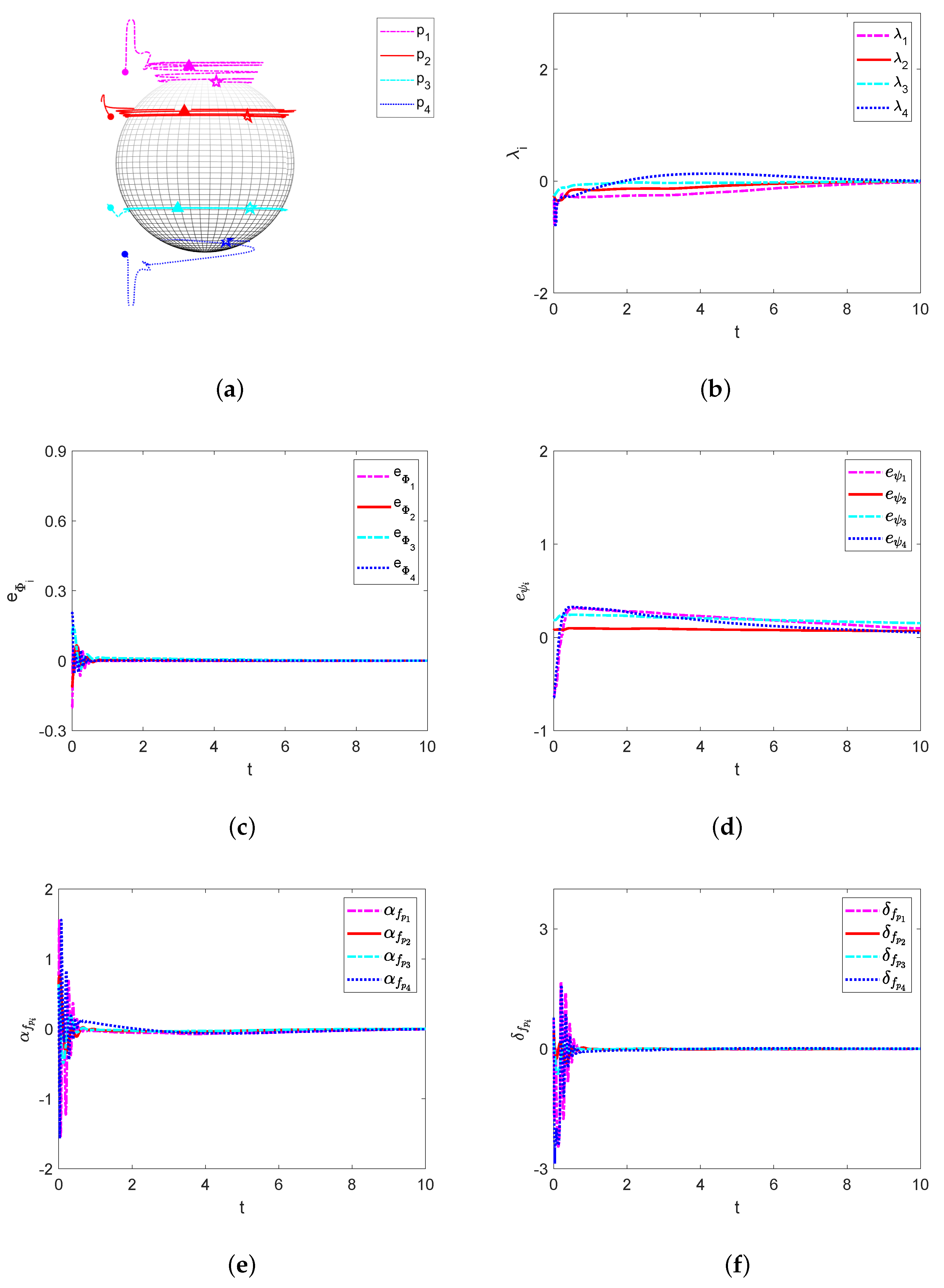
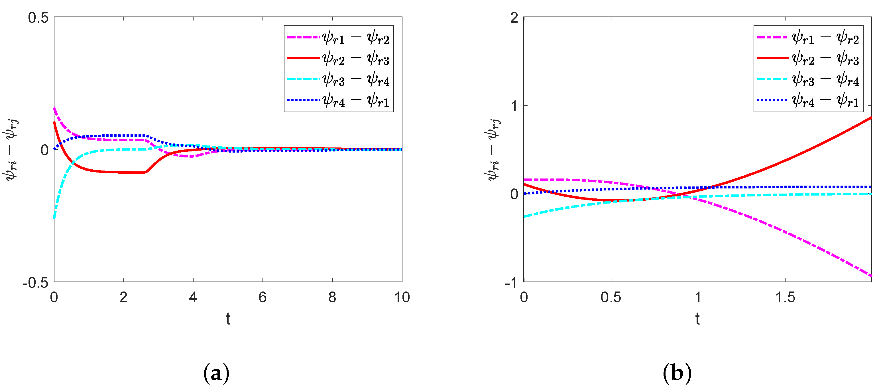
4. Simulation Results

In order to verify the effectiveness of the proposed spherical formation tracking control algorithm derived in Theorem 1 for dealing with the spherical formation tracking control problem with state constraints and time delays, a simulation example is given. The simulation example first demonstrates the spherical formation tracking motion, which aims to verify the implementation of the control objectives of sphere tracking, orbit tracking, orbital angles tracking, and the virtual-structure-like system tracking. Then, the formation motion is shown under different designs, which aim to verify the implementation of the formation based on the virtual-structure-like system. The simulation results verify the effectiveness of the proposed spherical formation tracking algorithm in Theorem 1.

Consider the directed network as shown in Figure 1. By the method of differential geometry, each follower tracks its planned orbits on a target sphere and forms a desired formation along the spherical orbits. The desired states related to the target sphere and the desired formation of four followers are given in the following description. For $i=1,2,3,4$, the fixed radius of the target sphere is ${\rho }_i=8$. The polar angles in the desired orbit of the target sphere are ${\varphi }_0^{\ast }=0$, ${\varphi }_1^{\ast }=\pi /3$, ${\varphi }_2^{\ast }=\pi /6$, ${\varphi }_3^{\ast }=0$ and ${\varphi }_4^{\ast }=-\pi /6$. The azimuthal angles associated with the desired line formation on the target sphere are ${\psi }_1^{\ast }=\pi /5$, ${\psi }_2^{\ast }=\pi /5$, ${\psi }_3^{\ast }=\pi /5$, and ${\psi }_4^{\ast }=\pi /5$.

Consider the dynamics of each follower in (3). In the process of simulation, the initial positions for four followers are

$$\begin{array}{c}\hfill {\left[p_{x1}\left(0\right),p_{y1}\left(0\right),p_{z1}\left(0\right)\right]}^T={\left[7,1,8\right]}^T,{\left[p_{x2}\left(0\right),p_{y2}\left(0\right),p_{z2}\left(0\right)\right]}^T={\left[7,6,4\right]}^T,\\ \hfill {\left[p_{x3}\left(0\right),p_{y3}\left(0\right),p_{z3}\left(0\right)\right]}^T={\left[7,6,-4\right]}^T,{\left[p_{x4}\left(0\right),p_{y4}\left(0\right),p_{z4}\left(0\right)\right]}^T={\left[7,1,8\right]}^T,\end{array}$$

and the initial pitch angles for four followers are ${\left[{\alpha }_1\left(0\right),{\alpha }_2\left(0\right),{\alpha }_3\left(0\right),{\alpha }_4\left(0\right)\right]}^T$$=[\pi /7,\pi /7,$${\pi /7,\pi /8]}^T$, and the initial surge velocities for four followers are ${\left[v_1\left(0\right),v_2\left(0\right),v_3\left(0\right),v_4\left(0\right)\right]}^T$$={\left[15,12,12,12\right]}^T$. The spatiotemporal flowfields are

$$\begin{array}{cc}\hfill & \left[\begin{array}{cccc}{f}_{p_{x1}}& f_{p_{x2}}& f_{p_{x3}}& f_{p_{x4}}\\ f_{p_{y1}}& f_{p_{y2}}& f_{p_{y3}}& f_{p_{y4}}\\ f_{p_{z1}}& f_{p_{z2}}& f_{p_{z3}}& f_{p_{z4}}\end{array}\right]\hfill \\ \hfill & =\left[\begin{array}{cccc}0.8& 0.9& 1.1+sint& 1.2+sin(p_{x4}^2+p_{y4})\\ 1.1& 1.2& 0.8+sin\left(2t\right)cost& 0.9+cos\left(p_{z4}\right)\\ 2.8& 2.8& 2.5+sint& 2.9+sin{p}_{z4}cos(p_{x4}^2+p_{y4}^2)\end{array}\right],\hfill \end{array}$$

and the maximum magnitude of $f_{li}$ is $f_M=4$. Since $v_{li}\left(0\right)=v_i\left(0\right)cos{\alpha }_i\left(0\right)$, $v_{li}\left(0\right)>f_{M_1}$ is obtained when choosing $f_{M_1}=\sqrt{5}{f}_M$. According to Remark 6, $v_{li}\left(0\right)>f_{M_1}$ yields $v_{f_{li}}\left(0\right)>2f_M$. ${\epsilon }_i=4$ is set for the position constraint (2) .

According to the spherical formation tracking algorithm given in Theorem 1, the control gains are selected as $c_1=10$, $c_2=10$, $c_3=5$, $c_4=6$, and $c_5=6$, and the time constants in the first-order filters are set as ${\tau }_1=0.001$ and ${\tau }_2=0.001$. The trajectories of four followers with different colors are shown in Figure 2a, where o, Δ, and ★ denote the different positions at $t=0\mathrm{s}$, $t=8\mathrm{s}$, and $t=10\mathrm{s}$, respectively. From this figure, four UAVs converge to the given orbits on the target sphere and form the formation with a sufficiently small neighborhood of zeros. The plots of ${\lambda }_i$, $e_{{\varphi }_i}$, $e_{{\psi }_i}$, ${\delta }_{f_{p_i}}$, and ${\alpha }_{f_{p_i}}$ are demonstrated in Figure 2b–f, respectively. Figure 2b–f shows that the control objectives of sphere tracking, orbit tracking, orbital angles tracking, and virtual-structure-like system tracking are achieved. A comparison is given to demonstrate the effectiveness of the formation with the virtual-structure-like design in (19). Figure 3a,b show that the formation with the proposed controller and non-delay controller that removing the term $f(({\psi }_{ri}-{\psi }_i^{\ast }),t)$ and delayed information, respectively. It is indicated that the proposed controller can yield the convergence of the formation but the formation associated with the non-delay controller divergences at $t\to \infty$. Consistently with Theorem 1, the spherical formation tracking control problem with state constraints and time delays is solved.

5. Conclusions

This paper deals with the spherical formation tracking problem of non-holonomic UAVs with state constraints and time delays. The state constraints include position and velocity constraints, and time delays existing in the directed communication network are time-varying. Since the tracking subsystem coupling with the formation subsystem, a novel virtual-structure-like design is proposed to achieve formation with time delays satisfying a more general assumption, which aims to transform the formation tracking problem into the tracking problem. The asymptotical stability of the virtual-structure-like system is obtained by virtue of the Lyapunov–Krasovskii functionals. In the simulation results, a comparison also demonstrates the effectiveness of the formation based on the virtual-structure-like design. Based on the virtual-structure-like design, the barrier Lyapunov functions are designed to develop a novel control scheme for tracking control and satisfy the position and velocity constraints for each UAV. A more simple manner for maintaining state constraints is given. The simulation results verify the effectiveness of the proposed spherical formation tracking algorithm.

Actually, input delays always occur in the feedback control loop, which is also called sensor-to-controller delay or controller-to-actuator delay. Different from time delays in the directed communication network, input delays have a delayed effect on the output of the controller. As a result, it can result in a delayed response from actuators. Input delays enable to make the system nonlinearity more complex, which results in many difficulties in stability analysis and controller design. In the future, it is of interest to solve the spherical formation tracking problem of non-holonomic UAVs with state constraints and input delays.

References

1. Li, R.; Shi, Y.; Song, Y. Localization and circumnavigation of multiple agents along an unknown target based on bearing-only measurement: A three-dimensional solution. Automatica 2018, 94, 18–25. [Google Scholar] [CrossRef]
2. Dou, L.; Song, C.; Wang, X.; Liu, L.; Feng, G. Target localization and enclosing control for networked mobile agents with bearing measurements. Automatica 2020, 118, 109022. [Google Scholar] [CrossRef]
3. Lin, J.; Song, S.; You, K.; Wu, C. 3-D velocity regulation for nonholonomic source seeking without position measurement. IEEE Trans. Control Syst. Technol. 2015, 24, 711–718. [Google Scholar] [CrossRef] [Green Version]
4. Chen, L.; Li, C.; Guo, Y.; Ma, G.; Zhu, B. Spacecraft formation-containment flying control with time-varying translational velocity. Chin. J. Aeronaut. 2020, 33, 271–281. [Google Scholar] [CrossRef]
5. Li, D.; Ma, G.; He, W.; Ge, S.; Lee, T. Cooperative circumnavigation control of networked microsatellites. IEEE Trans. Cybern. 2020, 20, 4550–4555. [Google Scholar] [CrossRef]
6. Yang, J.; Liu, C.; Coombes, M.; Yan, Y.; Chen, W.H. Optimal path following for small fixed-wing UAVs under wind disturbances. IEEE Trans. Control Syst. Technol. 2021, 29, 996–1008. [Google Scholar] [CrossRef]
7. Leonard, N.; Paley, D.; Lekien, F.; Sepulchre, R.; Fratantoni, D.; Davis, R. Collective motion, sensor networks, and ocean sampling. Proc. IEEE 2007, 95, 48–74. [Google Scholar] [CrossRef] [Green Version]
8. Lin, P.; Qin, K.; Li, Z.; Ren, W. Collective rotating motions of second-order multi-agent systems in three-dimensional space. Syst. Control Lett. 2011, 60, 365–372. [Google Scholar] [CrossRef]
9. Tan, Y.; Jin, Y. Multi-agent rotating consensus without relative velocity measurements in three-dimensional space. Int. J. Robust Nonlinear Control 2013, 23, 473–482. [Google Scholar]
10. Chen, L.; Mei, J.; Li, C.; Ma, G. Distributed leader-follower affine formation maneuver control for high-order multi-agent systems. IEEE Trans. Autom. Control 2020, 65, 4941–4948. [Google Scholar] [CrossRef]
11. Miao, Z.; Liu, Y.; Wang, Y.; Yi, G.; Fierro, R. Distributed estimation and control for leader-following formations of nonholonomic mobile robots. IEEE Trans. Autom. Sci. Eng. 2018, 15, 1946–1954. [Google Scholar] [CrossRef]
12. Lv, J.; Chen, F.; Chen, G. Nonsmooth leader-following formation control of nonidentical multi-agent systems with directed communication topologies. Automatica 2016, 64, 112–120. [Google Scholar]
13. Han, T.; Guan, Z.; Chi, M.; Hu, B.; Li, T.; Zhang, X. Multi-formation control of nonlinear leader-following multi-agent systems. ISA Trans. 2017, 69, 140–147. [Google Scholar] [CrossRef]
14. Rezaee, H.; Abdollahi, F. A decentralized cooperative control scheme with obstacle avoidance for a team of mobile robots. IEEE Trans. Ind. Electron. 2014, 61, 347–354. [Google Scholar] [CrossRef]
15. Liu, Y.; Gao, J.; Shi, X.; Jiang, C. Decentralization of virtual linkage in formation control of multi-agents via consensus strategies. Appl. Sci. 2020, 8, 2020. [Google Scholar] [CrossRef] [Green Version]
16. Do, K.; Pan, J. Nonlinear formation control of unicycle-type mobile robots. Robot. Auton. Syst. 2007, 55, 191–204. [Google Scholar] [CrossRef]
17. Ghabcheloo, R.; Pascoal, A.; Silvestre, C.; Kaminer, I. Coordinated path following control of multiple wheeled robots with directed communication links. In Proceedings of the 44th IEEE Conference on Decision and Control, Seville, Spain, 15 December 2005; pp. 7084–7089. [Google Scholar]
18. Peng, Z.; Wang, D.; Wang, H.; Wang, W. Distributed coordinated tracking of multiple autonomous underwater vehicles. Nonlinear Dyn. 2014, 78, 1261–1276. [Google Scholar] [CrossRef]
19. Zhang, F.; Leonard, N. Coordinated patterns of unit speed particles on a closed curve. Syst. Control Lett. 2007, 56, 397–407. [Google Scholar] [CrossRef] [Green Version]
20. Chen, Y.Y.; Chen, K.; Astolfi, A. Adaptive formation tracking control for first-order agents with a time-varying flow parameter. IEEE Trans. Autom. Control 2021, 67, 2481–2488. [Google Scholar] [CrossRef]
21. Chen, Y.Y.; Chen, K.; Astolfi, A. Adaptive formation tracking control of directed networked vehicles in a time-varying flowfield. J. Guid. Control Dyn. 2021, 44, 1883–1891. [Google Scholar] [CrossRef]
22. Zhao, S.; Dimarogonas, D.; Sun, Z.; Bauso, D. A general approach to coordination control of mobile agents with motion constraints. IEEE Trans. Autom. Control 2017, 63, 1509–1516. [Google Scholar] [CrossRef] [Green Version]
23. Liang, Y.; Dong, Q.; Zhao, Y. Adaptive leader–follower formation control for swarms of unmanned aerial vehicles with motion constraints and unknown disturbances. Chin. J. Aeronaut. 2020, 33, 2972–2988. [Google Scholar] [CrossRef]
24. Yu, X.; Liu, L. Distributed formation control of nonholonomic vehicles subject to velocity constraints. IEEE Trans. Ind. Electron. 2016, 63, 1289–1298. [Google Scholar] [CrossRef]
25. Wang, X.; Yu, Y.; Li, Z. Distributed sliding mode control for leader-follower formation flight of fixed-wing unmanned aerial vehicles subject to velocity constraints. Int. J. Robust Nonlinear Control 2021, 31, 2110–2125. [Google Scholar] [CrossRef]
26. Chen, Y.Y.; Tian, Y.P. Coordinated path following control of multi-unicycle formation motion around closed curves in a time-invariant flow. Nonlinear Dyn. 2015, 81, 1005–1016. [Google Scholar] [CrossRef]
27. Ai, X.; Chen, Y.Y.; Zhang, Y. Spherical formation tracking control of non-holonomic aircraft-like vehicles in a spatiotemporal flowfield. J. Frankl. Inst. 2020, 357, 3924–3952. [Google Scholar] [CrossRef]
28. Yong, K.; Chen, M.; Wu, Q. Constrained adaptive neural control for a class of nonstrict-feedback nonlinear systems with disturbances. Neurocomputing 2018, 272, 405–415. [Google Scholar] [CrossRef]
29. Liu, Y.J.; Zhao, W.; Liu, L.; Li, D.; Tong, S.; Chen, C.L.P. Adaptive neural network control for a class of nonlinear systems with function constraints on states. IEEE Trans. Neural Netw. Learn. Syst. 2021. [Google Scholar] [CrossRef]
30. Ghabcheloo, R.; Aguiar, A.; Pascoal, A.; Silvestre, C.; Kaminer, I.; Hespanha, J. Coordinated path-following in the presence of communication losses and time delays. SIAM J. Control Optim. 2009, 48, 234–265. [Google Scholar] [CrossRef] [Green Version]
31. Olfati-Saber, R.; Murray, R. Consensus problems in networks of agents with switching topology and time–delays. IEEE Trans. Autom. Control 2004, 49, 1520–1533. [Google Scholar] [CrossRef] [Green Version]
32. Tian, Y.P.; Liu, C. Consensus of multi-agent systems with diverse input and communication delays. IEEE Trans. Autom. Control 2008, 53, 2122–2128. [Google Scholar] [CrossRef]
33. Li, W.; Chen, Z.; Liu, Z. Leader-following formation control for second-order multiagent systems with time-varying delay and nonlinear dynamics. Nonlinear Dyn. 2013, 72, 803–812. [Google Scholar] [CrossRef]
34. Li, T.; Li, Z.; Shen, S.; Fei, S. Extended adaptive event-triggered formation tracking control of a class of multi-agent systems with time-varying delay. Neurocomputing 2018, 316, 386–398. [Google Scholar] [CrossRef]
35. Liu, K.; Xie, G.; Wang, L. Containment control for second-order multi-agent systems with time-varying delays. Syst. Control Lett. 2014, 67, 24–31. [Google Scholar] [CrossRef]
36. Wang, F.; Ni, Y.; Liu, Z.; Chen, Z. Fully distributed containment control for second-oder multi-agent systems with communication delay. ISA Trans. 2020, 99, 123–139. [Google Scholar] [CrossRef]
37. Li, D.; Liu, L.; Liu, Y.J.; Tong, S.; Chen, C.L.P. Adaptive NN control without feasibility conditions for nonlinear state constrained stochastic systems with unknown time delays. IEEE Trans. Cybern. 2019, 49, 4485–4494. [Google Scholar] [CrossRef]
38. Li, D.P.; Li, D.J. Adaptive neural tracking control for an uncertain state constrained robotic manipulator with unknown time-varying delays. IEEE Trans. Syst. Man Cybern. Syst. 2017, 48, 2219–2228. [Google Scholar] [CrossRef]
39. Sun, W.; Wu, Y.; Lv, X. Adaptive neural network control for full-state constrained robotic manipulator with actuator saturation and time-varying delays. IEEE Trans. Neural Netw. Learn. Syst. 2022, 33, 3331–3342. [Google Scholar] [CrossRef]
40. Liu, Y.; Zhu, Q. Event-triggered adaptive neural network control for stochastic nonlinear systems with state constraints and time-varying delays. IEEE Trans. Neural Netw. Learn. Syst. 2021. [Google Scholar] [CrossRef]
41. Ren, W.; Cao, Y. Distributed Coordination of Multi-Agent Networks; Springer: London, UK, 2011. [Google Scholar]
42. Khalil, H. Nonlinear Systems, 2nd ed.; Pearson Education Limited: Prentice Hall, Upper Saddle River, NJ, USA, 1996. [Google Scholar]
Figure 1. The communication topology in the virtual-structure-like system.
Aerospace 10 00118 g001
Figure 2. Spherical formation tracking motion with time delays: (a) spherical motion trajectories; (b) plot of λ i ; (c) plot of e ϕ i ; (d) plot of e ψ i ; (e) plot of α f p i ; (f) plot of δ f p i .
Aerospace 10 00118 g002
Figure 3. Formation in the case of (a) the proposed controller and (b) the non-delay controller.
Aerospace 10 00118 g003
Disclaimer/Publisher’s Note: The statements, opinions and data contained in all publications are solely those of the individual author(s) and contributor(s) and not of MDPI and/or the editor(s). MDPI and/or the editor(s) disclaim responsibility for any injury to people or property resulting from any ideas, methods, instructions or products referred to in the content.