Article

Aerodynamics and Power Balance of a Distributed Aft-Fuselage Boundary Layer Ingesting Aircraft †

Whittle Laboratory, University of Cambridge, Cambridge CB3 0DY, UK
*
Author to whom correspondence should be addressed.
This paper is an extended version of our paper published in Proceedings of the AIAA Propulsion and Energy 2020 Forum, Virtual Event, 24–28 August 2020.
Aerospace 2023, 10(2), 122; https://doi.org/10.3390/aerospace10020122
Submission received: 21 December 2022 / Revised: 18 January 2023 / Accepted: 19 January 2023 / Published: 27 January 2023
(This article belongs to the Section Aeronautics)

Abstract

:
This paper presents a first investigation into the aerodynamics and performance breakdown of a distributed aft-fuselage boundary layer ingesting (BLI) tube-and-wing aircraft using fully coupled Unsteady Reynolds-Averaged Navier-Stokes (URANS) calculations that resolve the complete fan and installation geometries. Through the URANS simulations, the interaction between the turbulence from the fuselage boundary layer (BL) and the BLI propulsor is identified as an area that warrants further research. Using the URANS approach, the ingested turbulence leads to a 4.5% reduction in the propulsor stage total–total isentropic efficiency. A mechanical power balance has been drawn up to compare the power sources and sinks throughout the installation and propulsor for two test cases with different thicknesses of ingested BL. The test case with a thinner BL was found to generate significantly more dissipation in the BL development upstream of the propulsor, the flow separation over the outer cowl, and the interaction between the reversed flow over the cowl and the propulsor exhaust jet. Due to this increase in dissipation, the case with thinner ingested BL consumes 7% more power relative to a baseline case with thicker BL, representative of the upstream fuselage at cruise. This demonstrates the importance of matching the installation with the incoming fuselage BL.

1. Introduction

Boundary layer ingestion (BLI) is a future aircraft technology that can potentially offer a step reduction in fuel burn by ingesting the airframe boundary layer with one or more aft-fuselage propulsors. The close integration between the airframe and propulsors requires a major change in the airframe design or modifications to the conventional tube-and-wing fuselage. Many different BLI concepts have been proposed, ranging from applying BLI to a new airframe concept [1,2,3] to modifying the conventional tube-and-wing fuselage with an additional single propulsor at the tail (propulsive fuselage concept) [4,5]. Nevertheless, it remains unclear what the most promising aircraft configuration for BLI is. The drawbacks from weight and component performance penalties, which may outweigh the aerodynamic benefits, depend greatly on the configuration. Although the fuel savings may not be as high since the fuselage accounts for about one fifth of the total drag [6], applying BLI to the conventional airframe poses less risk and has the potential to enter into service earlier, as it does not depend on a novel airframe.
In this study, the configuration-of-interest, depicted in Figure 1, features a conventional tube-and-wing fuselage with multiple aft-fuselage boundary layer ingesting (BLI) propulsors that are driven electrically. The under-the-wing gas turbine engines, besides generating thrust, drive generators to provide the required power for the BLI propulsors. Although this configuration is not able to ingest as much of the boundary layer as the propulsive fuselage concept, it is expected to fare better in non-aerodynamic areas such as weight, power system integration and noise [7]. Compared with the CENTRELINE propulsive fuselage concept [5], which uses an 8 M W motor for the BLI propulsor, a distributed BLI configuration significantly reduces the motor power rating P in each propulsor. This brings the power requirement in line with the projection of 1–3 M W for the non-cryogenic motor technology at Technology Readiness Level (TRL) 6 in 20 years’ time [8]. As the weight of conventional engines and motors scales with D f 2.4 [9] and P 1.5 [10], having multiple smaller propulsors will have a significant weight advantage over a large BLI fan. This also reduces the weights of the BLI fan containment system and additional airframe structures needed to support a rear propulsion system. Furthermore, the distributed propulsion system also allows independent control over the propulsors and thrust vectoring [11], which reduces the weight of the airframe control surfaces. This paper represents a first investigation into the aerodynamics of this novel configuration and first attempt to assess its aerodynamic performance.
The BLI benefit is sensitive to the fan efficiency reduction due to the inlet boundary layer; for instance, Plas et al. [12] found that a fan efficiency penalty of 2% and 1.3% excess loss in the inlet duct were sufficient to offset the 3–4% savings in power for the Silent Aircraft. Various studies on the fan aerodynamics report fan stage efficiency drops from 1–2% [13,14] to 10% [15], depending on the configuration-specific distortion profile and fan design. Therefore, it is equally important to assess the fan performance in this configuration.
This paper sets out to investigate the aerodynamics of the proposed aircraft concept through two computational test cases and analyse their performance using the power balance method, a mechanical power-based control volume method proposed by Drela [16]. The approach taken features Unsteady Reynolds-Averaged Navier-Stokes (URANS) computations on the combined aft-fuselage, installation and propulsor geometries. This allows the losses in both the installation and propulsor to be quantified and investigated.
Firstly, the Computational Fluid Dynamics (CFD) simulation set-up and power balance method are presented. Two test cases are introduced in Section 3: the first is a distributed aft-fuselage propulsor and installation at steady cruise ingesting a representative fuselage boundary layer, the second is the same configuration and flight condition, but with uniform flow at inlet to the computational domain. The paper compares the external flow field features of the cases and then investigates the impact of the ingested Boundary Layer (BL) on the propulsor. The later focus of the paper is on how the mechanical power balance is modified between the test cases and, in particular, how the useful recovered power terms and lost power through dissipation change throughout the installation and propulsion system. The use of the power balance method enables the changes in the internal and external flow field to be quantified by differences in the mechanical power input. This paper represents the first application of the power balance method to URANS computational results of a full-annulus BLI fan system combined with intake, exhaust system and upstream fuselage. It should be of interest to fan and installation engineers and researchers involved in the design of integrated fan and intake systems for BLI.

2. Computational Method

2.1. Computational Simulations

CFD simulations were carried out on Turbostream 3.6.3 [17], a GPU-accelerated, multi-block structured hexahedral grid, finite-volume Navier–Stokes solver with second-order spatial discretization, based on a cylindrical polar coordinate system. Turbulence is modelled using the RANS approach with the Boussinesq assumption of turbulent viscosity μ t , using the Spalart–Allmaras model [18] with helicity corrections [19]. The Spalart–Allmaras model has been used extensively in airframe simulations [20,21] and also other BLI fan studies [5,13,22]. Compared to other turbulence models, it is also less computationally expensive, and hence more suitable for large computations. The turbulent conductivity k t is estimated from μ t using the Prandtl number P r . Adaptive wall functions are used to model the wall shear stress. The flow over all surfaces is assumed to be fully turbulent. The computational grid has a maximum y + around 5, except on the exhaust nozzle casing and surfaces with separated flow. The installation and propulsor grids were generated using Pointwise V18.0R2 and NUMECA IGG/Autogrid5 11.2, respectively. It has a total of 306 million nodes, with 90 million in installation and 3.6 million nodes per rotor and stator blade row. The propulsor computational grid has more than twice the node count per blade in both blade rows, compared to the previous BLI fan aerodynamics study with the same solver by Gunn [14], which was based on the grid refinement study by Jerez Fidalgo [23]. A grid dependency study on the installation grid has been carried out, with the details in Appendix A. Although the boundary layer is axisymmetric due to the fuselage geometry, it is not the case for the distortion onto the propulsor, as the propulsor is not concentric with the fuselage, as illustrated in Figure 2. Due to the non-axisymmetric distortion, URANS calculations were carried out to resolve the propulsor internal flow and its interaction with the fuselage. Jameson’s dual time stepping scheme [24] was used with 2880 outer time steps per rotor revolution, similar to the value used in other BLI fan aerodynamics studies [13]. In the unsteady computations, sliding interfaces are used at the rotor–stator and rotor–installation boundaries to allow the rotor domain to rotate relative to the stator and installation grids. The time-averaged results are shown here unless otherwise specified. Further details of the solver and its numerical scheme can be found in Brandvik and Pullan [17].
The computational domain, centred around the fan-centric cylindrical polar coordinate system ( x , r , θ ), and the boundary conditions are shown in Figure 2. The computations have been performed on a 1/9th fuselage sector containing a single propulsor, with the use of slip walls to model the symmetry to save computational resources. This represents the simplified case of the fuselage at zero angle of attack. Since the computational domain only includes the rear half of the fuselage, a flow profile was prescribed at the inlet boundary. This involved setting the appropriate distributions of total pressure, total temperature and flow angles.

2.2. Application of Power Balance Method

In this section, the adaptation of the power balance method [16] for the fully-coupled computations is outlined. This allows for a more rigorous treatment of the rotating blades within the propulsor, which is more appropriate for this application, since the propulsor internal flow was resolved with the URANS approach. The control volume definition is presented first. This is followed by a discussion on the formulation, with the full derivation in Appendix B. The computational results were post-processed in ParaView 5.7.0 [25] with the in-built filters and the VTK library to implement the power balance method and streamline tracking. The turbulent fluxes were accounted for using the eddy viscosity μ t .

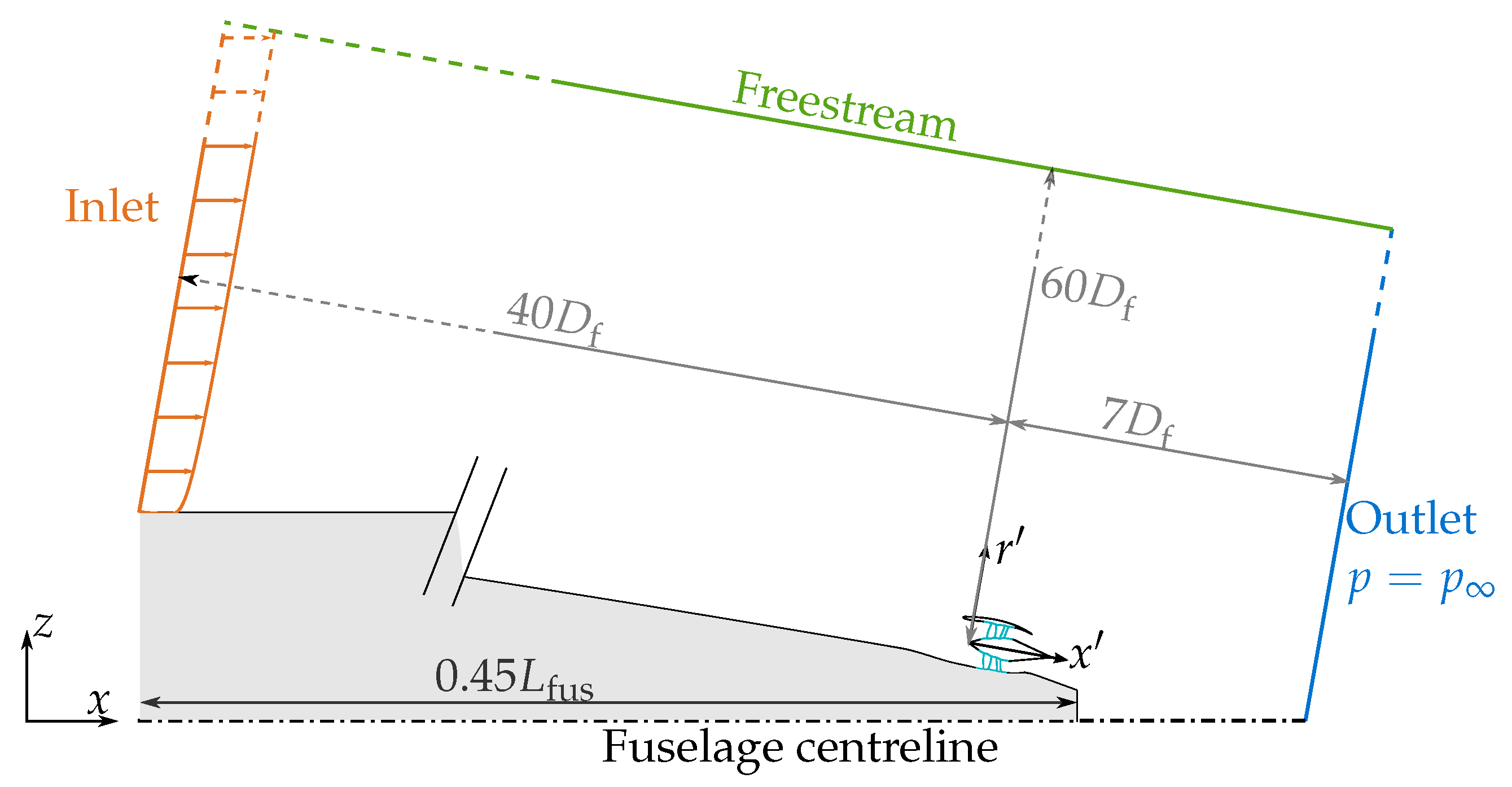
2.2.1. Control Volume

A typical control volume (CV) for the power balance is depicted in Figure 3. The CV V is bounded by several surfaces. The inlet and outlet set the axial extent of the CV. The radial extent is delimited by the freestream (FS) boundary, which can either be defined by a stream-surface, or as a general boundary that allows mass flux to cross it, similar to the inlet and outlet. In this study, a stream-surface freestream boundary, constructed by streamline tracking, was used.
Distinguishing among the different types of surfaces is important when drawing up a mechanical power balance for CV V , as a divergence theorem will transform some of the volume integrals into fluxes across these surfaces, which is outlined in the next section and Appendix B. Some of the integrals can be simplified by considering the relationship between the outward surface normal vector n ^ and the freestream and local velocity vectors V , V . In general, the surfaces can be divided into four categories: propulsor inlets and outlets S IO , prop , shown in blue in Figure 3; moving surfaces S MW , coloured in orange, with local wall velocity vector V MW (therefore V = V MW ); stationary viscous walls S FW where V = 0 (hence V · n ^ = 0 ); and external surfaces S ext , which are shown in red in Figure 3. The external surfaces S ext can be further classified into inlets, outlets and non-stream-surface freestream boundary ( V · n ^ 0 ); stream-surface ( V · n ^ = 0 , but V · n ^ 0 ); and side slip walls for modelling symmetry ( τ = 0 , V · n ^ = 0 , and due to slip wall alignment V · n ^ = 0 ). Note that even in the case V · n ^ = 0 , the work done from viscous stress τ ¯ ¯ · V · n ^ ( = τ ¯ ¯ · n ^ · V ) may not be zero, as the surface shear stress τ = τ ¯ ¯ · n ^ may not be perpendicular to V . The same argument applies for τ ¯ ¯ · V · n ^ 0 even when V · n ^ = 0 .

2.2.2. Formulation

In a steady or time-averaged periodic-unsteady flow field, the power balance for a CV V is given in Equation (1). The terms on the left hand side are power sources, which are balanced out by the sinks and outflows on the right. The full derivation and definitions of various terms are given in Appendix B.
P S + P V = V · F + all S ext ( E ˙ u + E ˙ p + E ˙ τ ) E ˙ + Φ
P S is the shaft power input—as the control volume V includes the propulsor with its moving blades, the propulsor power input can be evaluated by summing up the dot product between the force and velocity vectors around the rotor blades S MW . It can be shown, from the first law of thermodynamics, that this is also equal to the change in total enthalpy across the propulsor, provided all boundaries and walls are adiabatic and the work done from viscous stress on the propulsor inlet and outlet S IO , prop is negligible. This is a convenient way to side-step the integral on moving blades S MW in Equation (A7), i.e.,
P S = ( p p ) V + τ ¯ ¯ · V · n ^   d S MW = ( ρ V h 0 τ ¯ ¯ · V ) · n ^   d S IO , prop .
The shear stress contribution shaded in grey is usually small and was neglected in this study. Hence, the shaft power is insensitive to the placement of S IO , prop , as long as the CV bounded by it contains all S MW , since the total enthalpy should remain constant in the absence of heat transfer or further work input. As such, the shaft power P S used in this paper was evaluated using Equation (2) with the total enthalpy taken across the propulsor inlet and nozzle entry, which are shown in Figure 4b, to reduce the impact from CFD numerical scheme.
P V is the net pressure-volume power. It is the coupling between the mechanical and thermal energy, which is negligible for incompressible flow. The integrand for P V , ( p p ) · V , is related to the density gradient—if the flow, at a pressure higher than the freestream, is expanding, positive P V will be generated. In a compressible flow, the integrand ( p p ) · V is high locally, but as positive and negative regions usually appear side by side, the overall integrated quantity in CV is small.
On the sink side, V · F is the rate of work done by the net force F acting on the aircraft portion surrounded by the CV V . The next three E ˙ terms are the kinetic energy deposition rate due to velocity deviations from freestream E ˙ u , pressure work deposition rate E ˙ p and viscous stress work deposition rate E ˙ τ on the external boundaries. E ˙ τ is shaded because it is usually small at external boundaries unless the surface is within the fuselage BL as in the case of for a captured streamtube control volume.
Φ is the viscous dissipation rate within the CV, due to the work done by the viscous stress against the fluid deformation. With the (U)RANS approach, this term also accounts for the loss of mechanical energy to turbulent kinetic energy (TKE) production. It is a volume integral of the local dissipation rate per unit volume ϕ over V and is always positive. As adaptive wall functions are used by the solver to estimate the wall shear stress, the velocity gradients V in the first cell above the wall cannot be reliably calculated from the computed flow field. Consequently, the total viscous dissipation rate Φ in the CV cannot be accurately evaluated directly using Equation (A5). Instead, the total Φ is estimated indirectly by enforcing the mechanical power balance in Equation (1). A similar approach was used by [26,27]. Although the total Φ is better estimated from the power balance equation, the local ϕ should be unaffected by the wall functions for regions away from the wall.

3. Test Cases

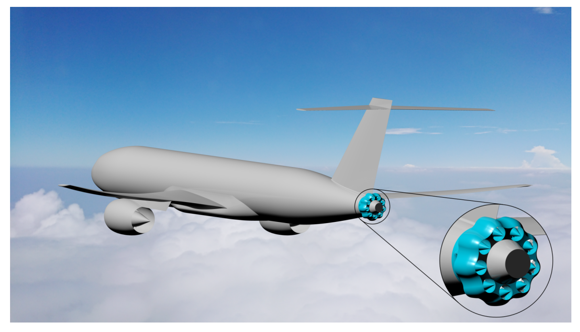
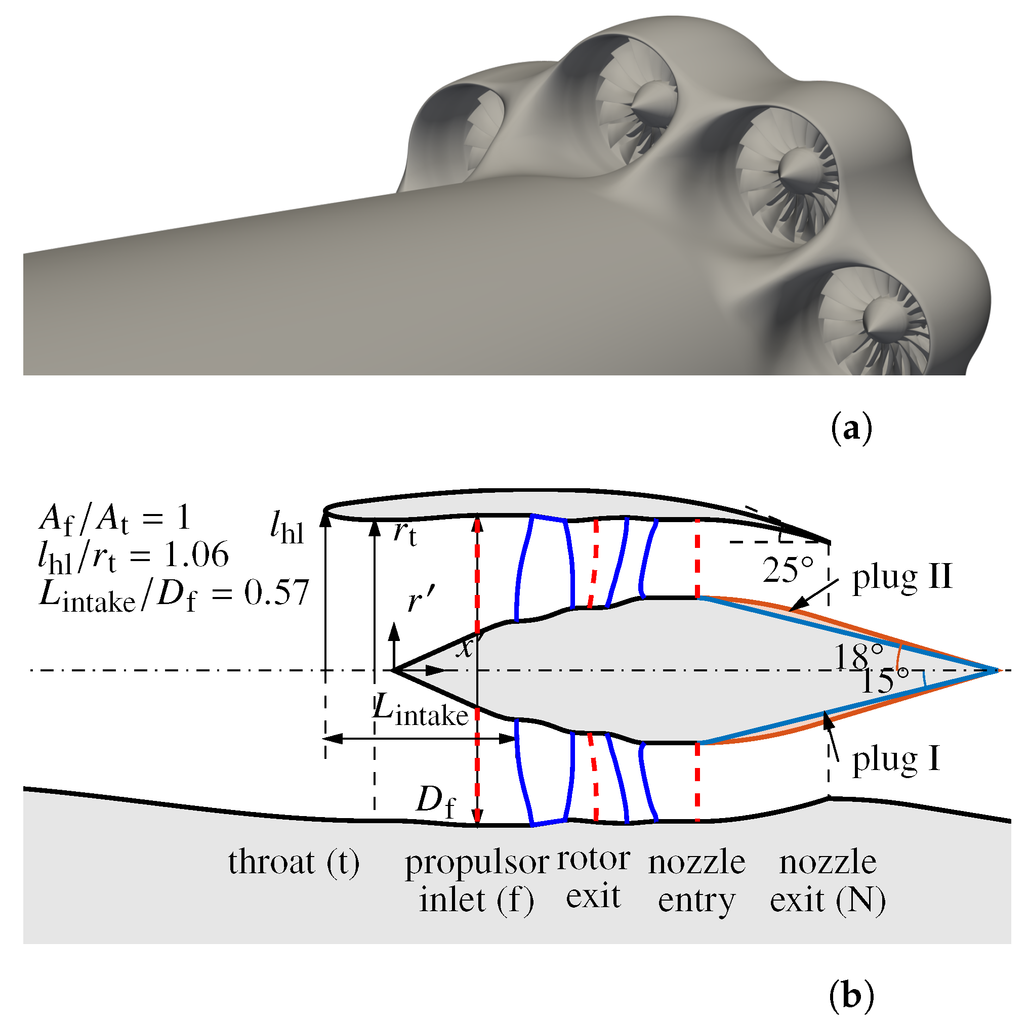
3.1. Installation and Fan Geometries

The test case geometry was assembled by adapting the fuselage and fan geometries from the literature. No attempts have been made to optimize the geometries. The fuselage is largely based on the NASA Common Research Model (CRM) [28], which is similar to a Boeing 777-200ER in size. To simplify the computational set-up, it is reduced to a body-of-revolution with a similar length-to-diameter ratio.
The installation of the BLI propulsors into the aft-fuselage were designed using computer-aided design (CAD) software. The intake was initially sized by considering continuity in 1D. Using the software’s in-built surface modelling, the surfaces were blended to minimise any surface discontinuities and to minimise the flow acceleration over the cowl. Figure 4a depicts the details of the intake geometry in 3D, which shows that the separating pillars between propulsors are slanted to reduce inlet distortion. The meridional view of the propulsor is shown in Figure 4b. The ratio of the propulsor inlet to throat areas A f / A t was set to 1 to prevent the inlet from choking and to limit the downstream diffusion between the throat and propulsor inlet planes. Between the throat and propulsor outlet, the internal geometry is axisymmetric around the fan rotational axis r = 0 .
Each propulsor is powered by a VITAL rotor [29], a low pressure ratio transonic fan, with a hub-to-tip radius ratio of 0.33 and rotor tip inlet relative Mach number of 1.2, which is representative of future gas turbine technologies. The stator and the annulus lines downstream of the rotor have been redesigned as the gas turbine core was removed. The fan is scaled in size to match the required fan diameter, with its rotational speed Ω adjusted to match the design normalised rotational speed N Ω . As the stator downstream is connected to the external flow via an exhaust nozzle, the only controls on the fan operating point are the shaft rotational speed Ω and nozzle area A N . The latter can be varied by changing the nozzle plug profile, as illustrated in Figure 4b.

3.2. Operating Conditions

Two computational test cases are presented in this paper. The CFD parameters are tabulated in Table 1. In the baseline case (case I), the inlet BL properties were extracted from a separate CFD simulation on the unpowered, non-BLI axisymmetric fuselage at the zero angle of attack. In the second case (case II), which simulates a uniform flow into the computational domain, the values are the same as the baseline apart from the stagnation pressure p 0 , which is uniform in this case. Case II can be interpreted as an aircraft with a shorter fuselage, or BLI with a lower ingested BLI fraction, i.e., some of the fuselage BL is diverted prior to the CFD domain. Alternatively, this can represent asymmetry in the fuselage BL caused by off-design conditions such as a high angle of attack. The details of the test cases are tabulated in Table 2, with the profiles of total pressure and Mach number at the domain inlet and centre plane displayed in Figure 5. The uniform p 0 profile at the inlet in case II leads to a BL with approximately half the displacement thickness δ * at 5 propulsor diameters upstream of the propulsor ( x ˜ = 5 ), as shown in Table 2.

4. Flow Field

Figure 6, showing the Mach number of the centre plane, highlights the main external flow features in both test cases. The flow structure is very different in case II, when the fuselage BL is thinner, especially in the flow over the cowl and in the exhaust region.

4.1. Fuselage Contraction

The development of the fuselage BL along the fuselage contraction is displayed in the velocity profiles in Figure 7, with the extent of the boundary layer indicated by the dashed lines. Along the contraction, the boundary layer thickens in both cases due to the diffusion in the adverse pressure gradient. The influence of the pressure field is also discernible in the BL edge velocity deviations from V in Figure 7. Near the propulsor inlet at x ˜ = 1 , the boundary layer is about 50% taller than the propulsor in case I, but comparable in size in case II, as indicated by the dashed δ / D f lines.

4.2. Cowl

In case I, there are two supersonic regions over the cowl at design, as shown by the isentropic Mach number distribution (Figure 8). The small supersonic bubble at the leading edge is caused by the incidence of the stagnation streamlines onto the cowl, as depicted in Figure 9. The cowl curvature causes the flow to accelerate just beyond sonic speed, resulting in a supersonic region with a peak Mach number of about 1.1. The flow is then returned to subsonic through a weak shock wave. The streamlines over the cowl in Figure 10a show that the flow remains attached over the cowl.
In case II, as the boundary layer is thinner, its mass flux ρ V x is higher, as depicted in Figure 9. Although the mass flow rate through the propulsor m ˙ f is 8% higher in case II, its captured streamtube has a smaller area. Consequently, the stagnation streamlines, which separate the internal and external flow, hit the inlet lip at a higher incidence, as shown in Figure 9. Due to the thinner BL, the flow approaching speed is also higher. These two factors lead to a higher acceleration around the cowl lip, which is reflected in Figure 8. This causes a large supersonic region in the front half of the cowl. The supersonic region terminates with a stronger shock wave at M 1.17–1.22, causing the flow to separate at the side slip walls, as clearly shown by the streamlines in Figure 10b, which are lifted off the cowl. The separation creates a large blockage, which pushes the cowl flow towards the centre, converging just above the exhaust jet at the trailing edge.

4.3. Exhaust Jet and After-Body

At the cowl trailing edge, flow separation is observed in both cases due to the sharp corner. The extent of the reversed flow region, measured by the axial velocity aligned with the propulsor V x , is indicated in Figure 11. As the flow remains attached up to the trailing edge in case I, the separation region is much smaller compared to case II. As the static pressure around the nozzle is governed by the point of separation, it is much lower in case II, since the flow separates at mid-cowl.
The jet velocity profile in Figure 12 shows that the distortion has not been fully attenuated across the propulsor. The top half of the exhaust jet is at a higher velocity, whilst the lower half of the jet leaves behind a wake further downstream, which is also evident in Figure 6. The exhaust jet is very different between the two cases. In case I, the exhaust nozzle is not close to choked, unlike conventional jet engines. This is because the inlet total pressure is much lower than the freestream stagnation pressure at M = 0.85 due to the fuselage boundary layer. In case II, there is a full-annulus supersonic region at the nozzle exit, as depicted in Figure 6b, suggesting that the nozzle is choked. As the pressure ratio across the fan remains similar, as it will be shown in Figure 13, but the stagnation pressure p 0 is higher at the propulsor inlet due to the thinner boundary layer, the p 0 at nozzle exit is higher, with the mass-averaged value at 1.90 p . This is 7% higher than the case I value. Combining with the low pressure region surrounding the jet, the total-to-static pressure ratio is sufficiently high to cause choking. As the condition for choking only depends on the pressure ratio at the nozzle exit plane, the nozzle area merely sets the mass flow through the propulsor. To match the fan operating point, case II has a 5% smaller nozzle area, which leads to a steeper nozzle plug angle, as shown by the plug profiles in Figure 12.
Due to the fuselage contraction, the propulsor is angled relative to the fuselage axis. Consequently, the exhaust jet exits at an angle of about 10°. As this is an axisymmetric configuration, the jet will eventually be turned to align with the fuselage axis as the transverse momentum from the jets cancels out. The jet realignment is depicted in Figure 12, along with the high pressure region established behind the aircraft to turn the jet. Due to the stronger jet, a larger high pressure region with greater back pressure is established in case II, which leads to the quicker deceleration of the exhaust jet, as observed in Figure 6. The back pressure would also encourage a reversed flow onto the cowl, leading to the larger separated flow region observed in Figure 11. The separation point will be a balance between the back pressure and incidence onto the cowl as the shock strength is set.

4.4. Fan Aerodynamics

Figure 13 shows the operating points of the propulsor in the two test cases. As illustrated in Figure 4b, the nozzle area A N in case II has been reduced by 5% relative to case I to match the fan operating point, as the flow speed approaching the propulsor is higher in the former case. Nevertheless, since the p 0 , f is higher, the mass flow through the propulsor m ˙ f is 8% higher in case II, as shown by the intake flow ratio in Table 2.
Compared with the operation in the uniform inlet flow with p 0 = p 0 , (⋄) shown in Figure 13, obtained from a 1/6th annulus URANS calculation with the same propulsor mesh, the fan stage suffers from a 6.6% drop in total–total efficiency η tt and a 2.3% reduction in total–total pressure ratio r p in case I (Δ).

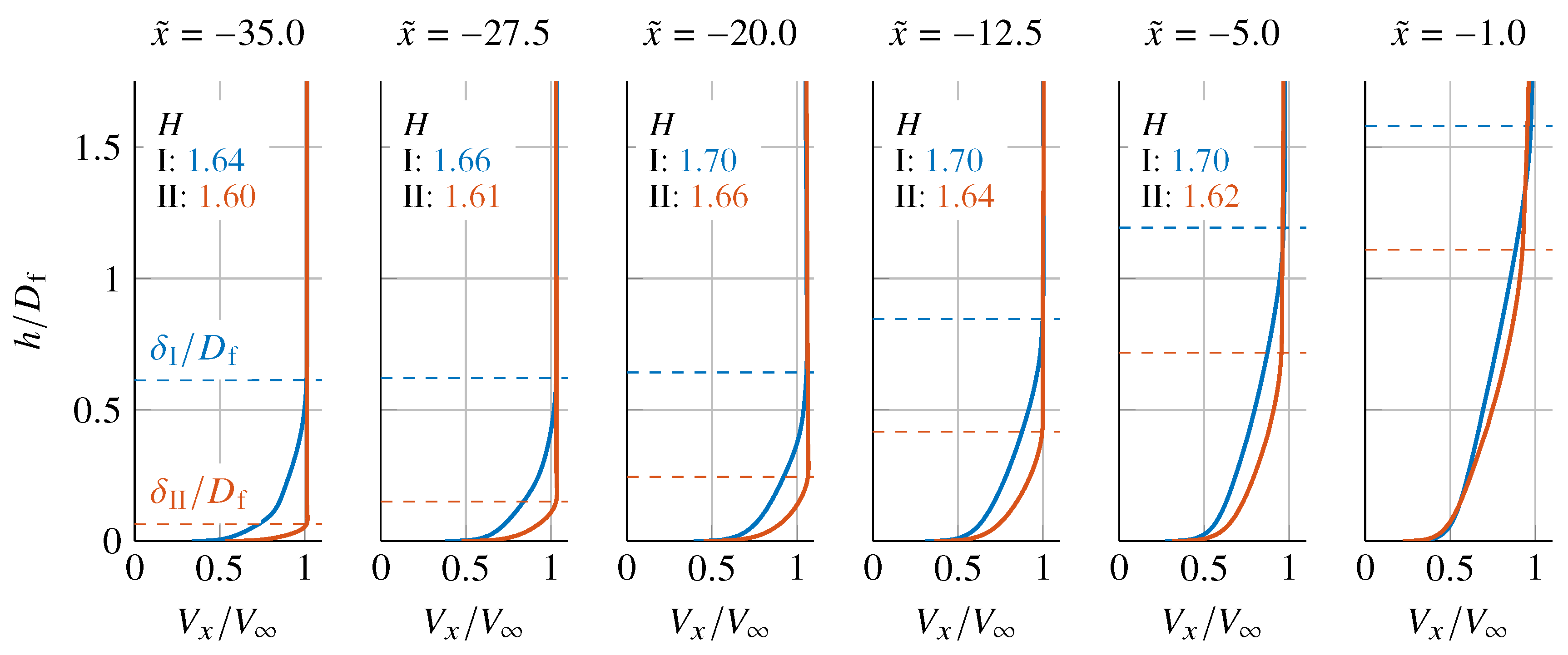
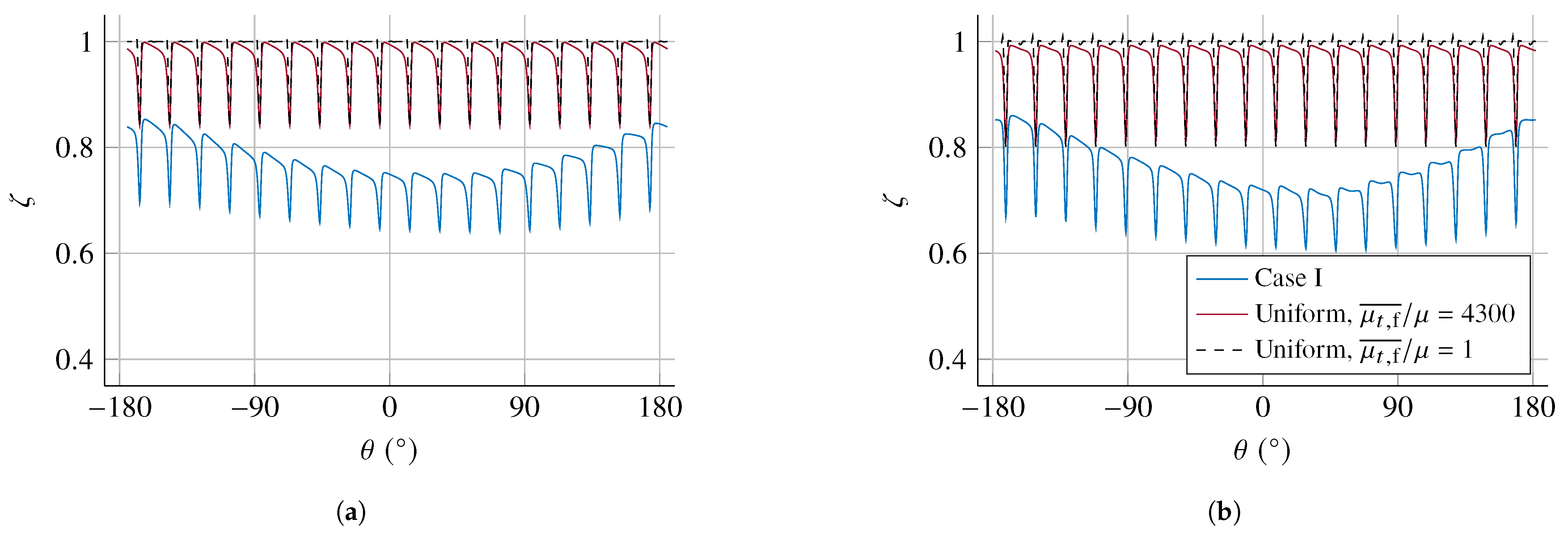
4.4.1. Effect of Fuselage BL Turbulence

As the BL develops along the fuselage, turbulence is also produced through shear, in additional to the total pressure distortion shown in Figure 14a. With the URANS approach using a linear viscosity turbulence model, the turbulence is manifested as a very high eddy viscosity μ t . This leads to a high level of turbulent viscosity ratio μ t / μ , of the order 10 3 , at the propulsor inlet, as depicted in Figure 14b. The mass-averaged eddy viscosity ratio at the propulsor inlet μ t , f ¯ / μ is about 4300.
To illustrate the effect of high inlet turbulence, two fan-only, URANS test cases were set up with uniform inflow, i.e., p 0 = p 0 , : one represents the podded propulsor, which has a low inlet turbulence level μ t , f ¯ / μ = 1 (⋄), whilst the other has μ t , f ¯ / μ = 4300 (). The fan performance of these two cases are also shown in the fan map in Figure 13. At constant Q f , the high inlet turbulent viscosity leads to a 1.5% reduction in r p and 4.5% in η tt , which is indicated by the i-arrow in Figure 13. Hence, a significant proportion of the drop in η tt between the uniform inflow, low μ t , f and BLI cases, which is indicated by the iii-arrow in Figure 13, can be attributed to the high inlet turbulence.
The high effective viscosity μ eff = μ + μ t seen by the solver leads to increased dissipation as the flow is smoothed out. The rate of mechanical energy loss is quantified by the local dissipation generation per unit volume ϕ = ( τ ¯ ¯ eff · ) · V = ( μ + μ t ) [ V + ( V ) T ] : ( V ) . With the (U)RANS approach, this term accounts for both the conversion of mechanical energy to thermal energy due to the work done against fluid deformation by the viscous stress, and the loss of mechanical energy to TKE production. Hence, the high μ eff increases the rate of loss of mechanical energy ϕ substantially. From the RANS perspective, the high eddy viscosity implies an increased rate of mechanical energy leaving the mean field to TKE production, as the turbulence increases the mixing.
Figure 15 shows the entropy function relative to freestream ζ = exp [ ( s s ) / R ] at the rotor downstream for two span fractions. In the BLI case, the total pressure distortion leads to an offset and circumferential variation in ζ , as the BL leads to a p 0 smaller than p 0 , at the propulsor inlet. Nevertheless, apart from that the overall wave-like variation, the local ζ profile is similar to that for the uniform inflow μ t , f ¯ / μ = 4300 case. Hence, the effect of BL turbulence can be isolated by comparison between the two uniform inflow cases at different μ t , f ¯ / μ levels. At μ t , f ¯ / μ = 4300 , the ζ is lower at mid-passage. This suggests that the entropy is much higher, compared to μ t , f ¯ / μ = 1 . As the inflow is uniform, ζ = 1 at the rotor inlet. Therefore, the mid-passage loss is much higher in the elevated viscosity case, which is otherwise negligible when μ t , f ¯ / μ = 1 , since the flow should be near-isentropic away from the blade surfaces and endwalls. The wakes in μ t , f ¯ / μ = 4300 and BLI cases are also much smoother due to the increased mixing from the turbulence.
Although (U)RANS was used extensively to resolve the fan flow field with total pressure and/or swirl distortions at the inlet [13,15,31,32,33] and the flow over airframe [20,21], it is unclear whether URANS can accurately model the effects of the turbulent structures from the fuselage BL on the fan internal flow. URANS calculations require the existence of a spectral gap, i.e., the turbulence time and length scales should be much smaller than those corresponding to the unsteadiness resolved by the unsteady time-stepping scheme [34]. In the coupled calculations in this paper, the size of the largest turbulent eddies in the fuselage BL is comparable to the fan diameter. Consequently, as Tucker [34] has shown for BLI engines, a reverse spectral gap may arise. Therefore, whilst the small BL eddies can be modelled with RANS turbulence models, the large ones should be resolved as unsteadiness entering the fan, which changes its operating point, instead of treating them as an increased effective viscosity with the Boussinesq assumption. This is essentially the hybrid RANS–Large Eddy Simulation (LES) approach.
Considering the uncertainty about the accuracy and validity in the (U)RANS prediction on the effects due to the ingested turbulence, the fan characteristics in Figure 13 provide the upper and lower bounds of the efficiency impact. The worst case is the current approach of modelling all of the turbulence as dissipative eddy viscosity, leading to a Δ η tt of 6.6%, as indicated by the iii-arrow. Meanwhile, the best case is following the common assumption in past BLI fan aerodynamics studies that the adverse impact from the fuselage BL turbulence is minimal. This corresponds to the comparison at the same μ t , f ¯ / μ , as indicated by the ii-arrow, with a Δ η tt of 2.1%, which is comparable to the efficiency drop reported by Gunn [14].

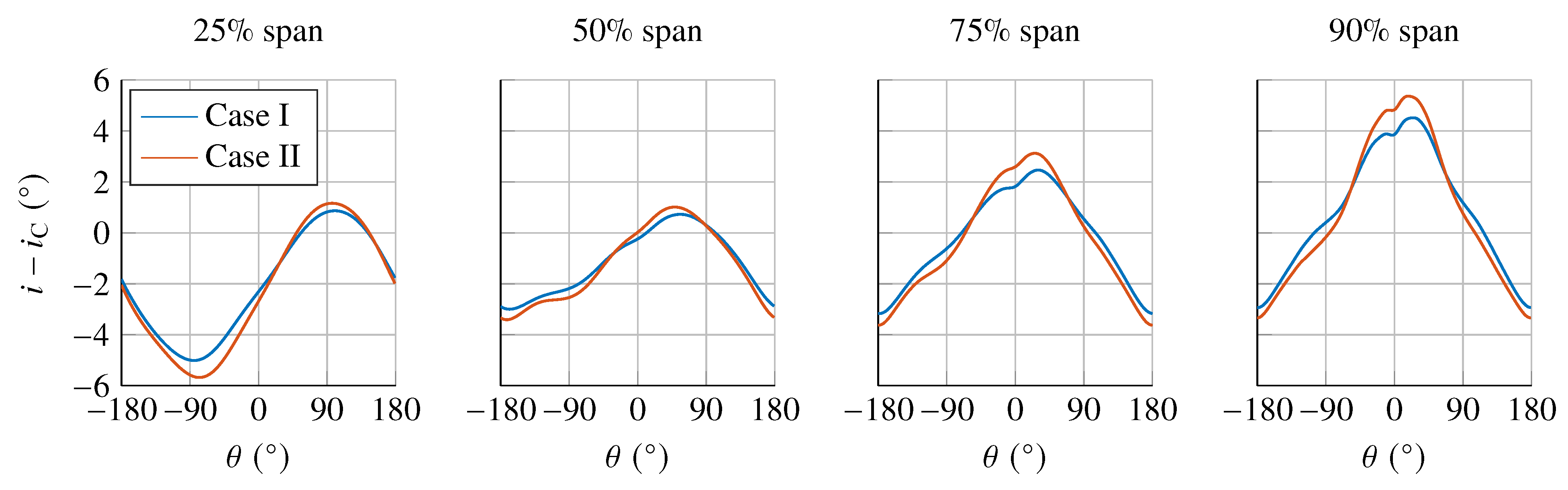
4.4.2. Inlet Distortion

The stagnation pressure at the propulsor inlet for case I is shown in Figure 14a. As the propulsor is only ingesting part of the boundary layer, the peak p 0 , f / p 0 , is only 87% near θ = 180 . Whilst the total pressure drop from the inlet lip to propulsor inlet is only 0.3%, the overall recovery relative to freestream ( p 0 , f ¯ / p 0 , ) is only 79%. As the propulsor is submerged in the boundary layer, this leads to a total pressure distortion covering the full propulsor inlet in both cases, with non-uniformity in both radial and circumferential directions. The thinner boundary layer in case II raises the stagnation pressure at the propulsor inlet, with a mass-averaged p 0 , f ¯ / p 0 , of 85%.
The change in incidence at the propulsor inlet, relative to the reference operating point in the uniform flow in Figure 13, due to the inlet distortion is shown in Figure 17. Despite the difference in the inlet total pressure, the change in incidence remains similar between cases I and II. Comparing the results at various span locations in Figure 17 shows maximum differences of about 1°, whilst the overall flow mechanism remains unchanged. This is because the fan operating point is similar between the two cases through the use of different exhaust nozzle plugs. Therefore, the remaining section will focus on the internal flow field in case I.

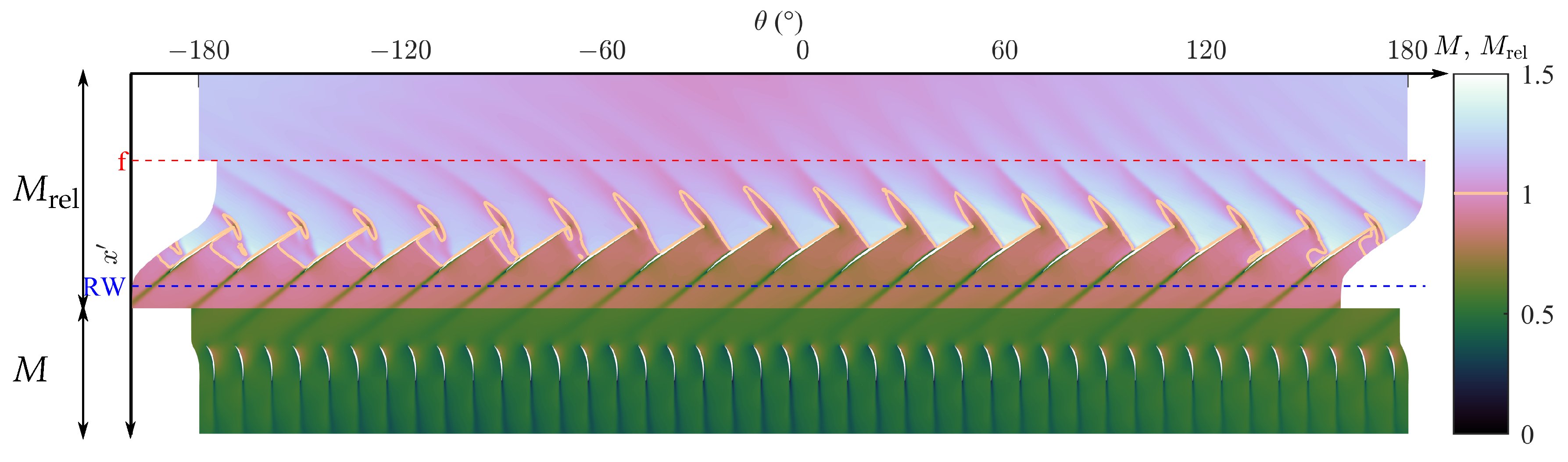
4.4.3. Internal Flow Field

In this configuration, the rotor blade tip experiences a large swing in incidence as it completes one revolution. This change in operating condition is also reflected in the instantaneous flow field in Figure 16, where the rotor passages exhibit a range of behaviour. As identified by Gunn and Hall [13], the flow redistribution ahead of the propulsor leads to regions of co-swirl ( θ < 0 ° ) and counter-swirl ( θ > 0 ° ). The lower mass flux in the low momentum region ( θ = 0 ° in Figure 14a) leads to an increased incidence onto the blades. Combined with the counter-swirl flow, which also acts to increase the incidence, this leads to a region of expelled shocks, similar to the behaviour near stall in θ < 90 ° . On the other hand, the co-swirl flow counteracts the increased incidence due to the low mass flux in θ < 0 ° . Therefore, the passages gradually move towards choked, which starts at around θ = 90 ° , as indicated by the swallowed passage shocks. At the high momentum region near θ = ± 180 ° , the passages are choked.
The entropy function ζ at the rotor exit in Figure 15 is a measure of the entropy increase relative to freestream conditions p and T . As the inlet distortion is symmetric around θ = 0 ° , it can be concluded that the loss within the rotor is higher in the counter-swirl region ( θ > 0 ° ).

5. Mechanical Power Balance

To understand the performance of this aircraft configuration, mechanical power balances were drawn up for the time-averaged URANS solutions as described in Section 2.2. This allows the propulsor shaft power P S to be broken down into the various power sources, sinks and in/outflows in the control volume. Figure 18 shows the power balances for both test cases with the CV V in Figure 3. The terms are normalised by q V S ref to form power coefficients C ( A ) , where q = 1 2 ρ V 2 is the freestream dynamic head and S ref is the reference area of 4130 ft2 [20]. Typically, only about 80% of the propulsor shaft power P S is converted into useful mechanical power input into the external flow field. The rest is converted into viscous dissipation Φ (which also includes TKE production as discussed in Section 4.4.1) and net pressure-volume power P V within the propulsor domain, which is bounded by the blue S IO , prop planes in Figure 3. The overall P V is small in the control volume V , which includes both internal and external flows.
V · F represents the rate of work done by the net force F on the aircraft portion surrounded by CV V , as the aircraft travels at V . When the force F is in the opposite direction to V in the aircraft reference frame, it represents surplus power, in the form of thrust, available to propel other parts of the aircraft. On the contrary, if it appears on the source side, i.e., F acting in the same direction as V , as in case II, then the BLI propulsor is not sufficient to propel the section of aircraft surrounded by the CV. Therefore, extra thrust is required from the other parts.
The inlet E ˙ = E ˙ u + E ˙ p + E ˙ τ usually appears on the source side. The velocity non-uniformity in the upstream boundary layer is a power source through E ˙ u , because it follows the same direction as the local velocity. In the absence of a reversed flow, any velocity deviations from the freestream always deposit their energy into the CV at the inlet. The static pressure is below p due to the fuselage geometry at the CV inlet. Hence, within the boundary layer, this leads to an inflow for E ˙ p . However, outside of the boundary layer, the low pressure causes the flow to speed up relative to V , which will lead to E ˙ p flowing out of the CV in that area. Therefore, whether the overall E ˙ p for the inlet plane flows into or out of the CV depends on the extent of the plane. The deposition rate due to viscous stress, E ˙ τ , is small as the component of shear stress acting on that face τ = τ ¯ ¯ · n ^ along the V V direction predominantly depends on the streamwise velocity gradient, which is small, compared to the gradient up to the boundary layer. Comparing between the two cases, the corresponding inlet E ˙ u + E ˙ p + E ˙ τ is much lower in case II because the inlet boundary layer is thinner, leading to lower power input from the velocity deficit. Moreover, as the inlet plane captures more freestream flow, this leads to an outflow of E ˙ p .
At the outlet, the jet and wake deposits energy out of the CV in E ˙ u , which is partially offset by the inflow from E ˙ p . The overall pressure defect work is a balance between the jet ( E ˙ p outflow) and wake ( E ˙ p inflow) regions. The net E ˙ outflow is a lost work, as it is not recovered downstream of the aircraft. As observed in Figure 6, the jet mixes out quicker in case II, which explains the smaller E ˙ flux at the outlet.
At the freestream stream-surface (FS), E ˙ u = 0 , as the no-mass fluxes crosses it. As it is outside of the fuselage BL, E ˙ τ 0 . However, due to the pressure field of the fuselage, it transfers a net E ˙ p energy out, as the outflow from the low pressure region outweighs the inflow in the high pressure area towards the end of the aircraft.
The viscous dissipation rate Φ is a measure of the rate of mechanical energy lost to thermal energy through the work done by viscous stress, and to TKE production. As this conversion is one-way, the local generation is always positive. Since it is a volume integral, the total dissipation can be broken down into contributions from various regions, as defined in the inset in Figure 18. In both cases, the dissipation within the propulsor (region D) accounts for about 16% of the shaft power.
Comparing the power balances in Figure 18 between two test cases shows that the C Φ in case II is 66% higher than that in case I—in fact, in the thinner BL case, the total dissipation in the installation and propulsor amounts to over 90% of the shaft power. According to the dissipation breakdown, the greatest increase in C Φ magnitude occurs in region C, the exhaust region, due to the large area of separated flow, which extends close to the jet. The local ϕ distribution is useful for identifying the regions with high losses. In Figure 11, the shaded high ϕ region ( C ϕ D f 3 3 e 4 ) overlaps with the isoline of V x = 0 (Aerospace 10 00122 i002
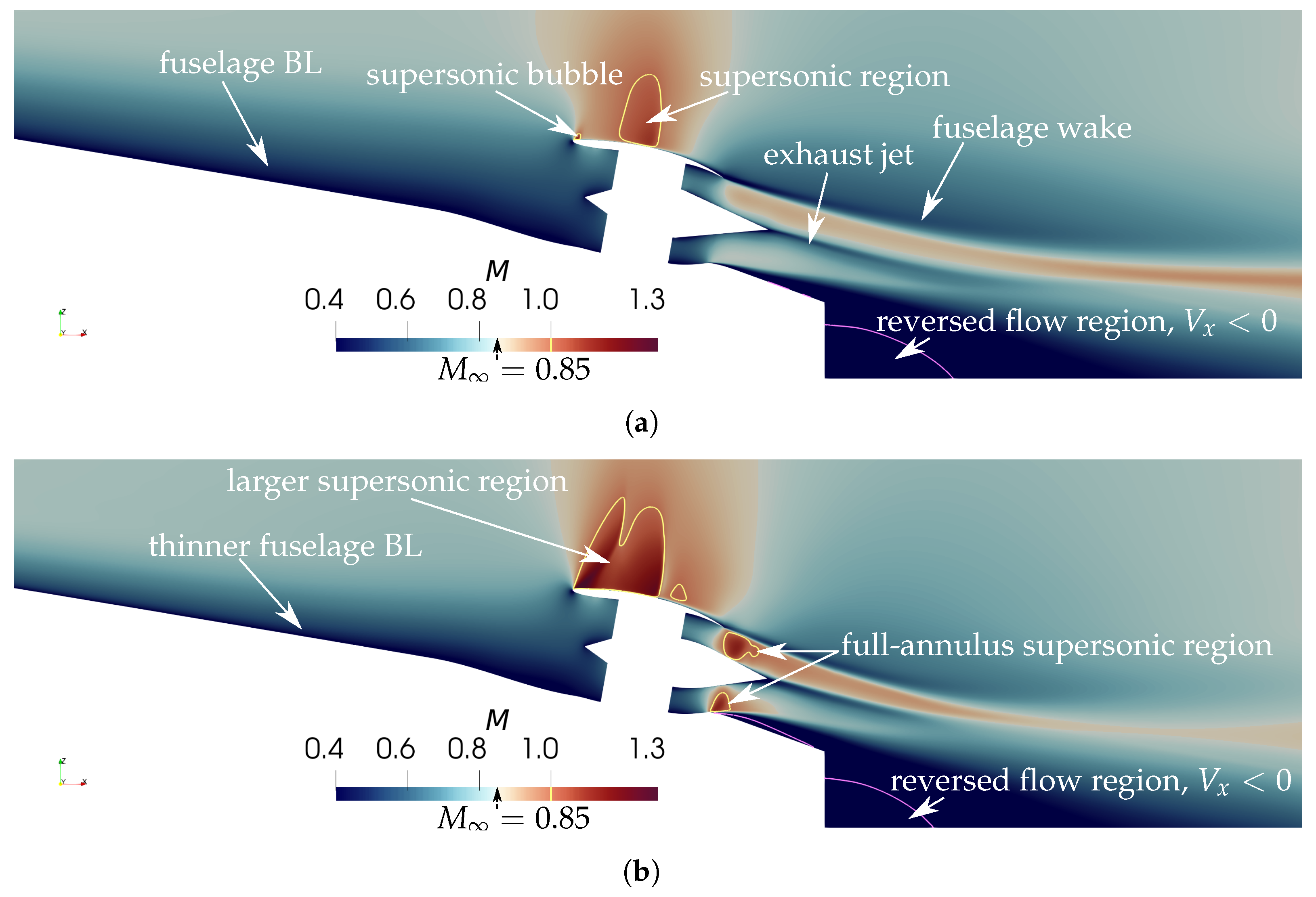
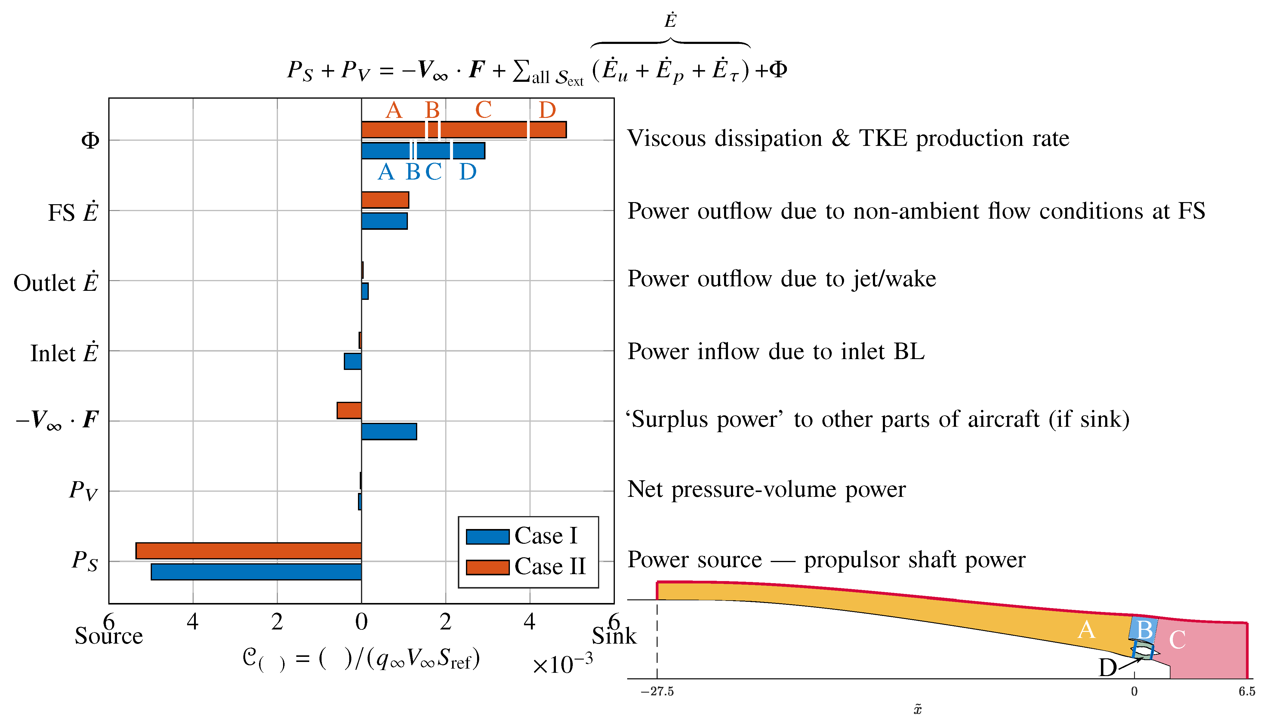
). This implies that the reversed flow takes part in the mixing with the jet, which has a higher velocity than case I. The higher velocity gradient increases the shear stress and, therefore, dissipation. The stronger shock and flow separation over the cowl has approximately tripled the dissipation in region B, but the contribution to the total dissipation remains small. Down the fuselage ramp, the dissipation also increases because the velocity gradient is higher in the thinner boundary layer.
The increase in dissipation in case II is the main cause for its V · F deficit. It is the flow field set up by the thinner boundary layer that leads to poorer performance in case II, instead of the lower power inflow at the inlet due to the lower velocity deficit in the thinner inlet BL. Therefore, through improved design of the cowl and the after-body to match the incoming boundary layer, the performance can be improved.
As aforementioned, V · F can be interpreted as the surplus power, in the form of extra thrust, available to the aircraft portion not surrounded by V . Using the drag coefficient of the CRM Complete Cruise Configuration of 306.8 dc [35], the drag of a typical conventional aircraft can be estimated. The drag D u of the aircraft portion outside of V , in cases I and II are assumed to be the same (To estimate D u , the portion of drag at x ˜ > 27.5 for the unpowered, non-BLI axisymmetric fuselage mentioned in Section 3.2 is subtracted from the total CRM drag). To estimate the thrust required from the main under-the-wing engines, the thrust surplus in the CV V for a full-annulus of nine BLI propulsors, i.e., N = 9 , using V · F in Figure 18, is subtracted from D u . The main engines in all cases are assumed to be powered by the VITAL fan operating at the reference point (⋄) in Figure 13, with different sizes, and therefore mass flow rate, to match the thrust requirement at cruise, i.e., zero net axial force. The total shaft power is estimated by summing the BLI propulsors’ P S and that from the main engines. Compared with case II, case I consumes 7% less total shaft power.

6. Conclusions

This paper demonstrated the flow field for this novel distributed BLI propulsion concept using two test cases with different incoming boundary layer thicknesses: one representative of the fuselage BL at cruise, and the other with a thinner BL. This led to two distinct modes of external flow structure. A thinner fuselage boundary layer leads to increased incidence and flow speed onto the cowl. This influences the cowl shock structure and impacts the flow separation and downstream viscous dissipation generation in the exhaust jet, and consequently the performance. The interaction between the flow separation at the cowl trailing edge and the exhaust jet leads to high viscous dissipation, and therefore poor BLI performance. Through improved design over the cowl and near the exhaust area, the loss generation could be reduced.
The inclusion of full fan geometry in the URANS set-up allows the impact of the fuselage BL on the fan to be studied. With the linear viscosity turbulence model, all of the fuselage BL turbulence were modelled as eddy viscosity. This leads to a much higher total–total efficiency penalty between the podded and BLI fan stages, compared to other BLI studies, which neglected the ingested turbulence. Under the URANS approach, the ingested BL turbulence leads to a 4.5% reduction in the stage total–total isentropic efficiency. As there are great uncertainties in the extent of the adverse impact of the fuselage BL turbulence on fan aerodynamics and performance, it is important to de-risk it with further investigations using experiments and computations.
Mechanical power balances were drawn up to assess the performance. This enables a breakdown of the useful mechanical power throughout the installation and propulsion system. When scaled to a full aircraft, the thinner inlet boundary layer case requires 7% more shaft power compared to the baseline case. This difference is mainly caused by the increase in viscous dissipation in the BL upstream of the propulsor, in the flow over the cowl and in the separation in the exhaust jet. This highlights the importance of matching the cowl and after-body design to the fuselage boundary layer.

Author Contributions

Conceptualization, T.S.T. and C.A.H.; methodology, T.S.T. and C.A.H.; software, T.S.T.; validation, T.S.T.; formal analysis, T.S.T.; investigation, T.S.T.; resources, C.A.H.; data curation, T.S.T.; writing—original draft preparation, T.S.T.; writing—review and editing, T.S.T. and C.A.H.; visualization, T.S.T.; supervision, C.A.H.; project administration, C.A.H.; funding acquisition, C.A.H. All authors have read and agreed to the published version of the manuscript.

Funding

This research was funded by Rolls-Royce plc and EPSRC under the Centre for Doctoral Training in Gas Turbine Aerodynamics (EP/L015943/1) with a reference number 1799072.

Institutional Review Board Statement

Not applicable.

Informed Consent Statement

Not applicable.

Data Availability Statement

Not applicable.

Acknowledgments

The authors would like to thank Rolls-Royce plc and the EPSRC for funding this work. T.S.T. was also financially supported by the Cambridge Trust and Magdalene College, Cambridge. Turbostream Ltd., UK, is acknowledged for making their solver, Turbostream 3.6.3, available and the support, particularly from Ewan Gunn. Alejandro Castillo Pardo, Nixon Ma and Lachlan Jardine are thanked for the thought-provoking discussions. Tim Williams is thanked for providing his blade design tool for the propulsor redesign work. This work was performed using resources provided by the CSD3 operated by the University of Cambridge RCS, provided by Dell EMC and Intel using Tier-2 funding from the EPSRC (capital grant EP/P020259/1), and DiRAC funding from the STFC.

Conflicts of Interest

The authors declare no conflict of interest.

Nomenclature

AArea
AArea of the captured streamtube at upstream freestream condition, i.e. m ˙ f = ρ V A
AtArea at the intake throat
C (   ) Power coefficient, C (   ) = (   ) / ( q V S ref )
DfPropulsor diameter at propulsor inlet
E ˙ Mechanical energy deposition rate
E ˙ τ Viscous stress work deposition rate
E ˙ p Pressure work deposition rate
E ˙ u Kinetic energy deposition rate
FNet force acting on the aircraft portion surrounded by the control volume
HBoundary layer shape factor
hHeight from surface
h0Specific total enthalpy
iIncidence angle, positive if stagnation point is on blade pressure surface
LfusFuselage length
lhlDistance between intake highlight and propulsor rotational axis
LintakeIntake length
m ˙ Mass flow rate
M; MrelMach number; Mach number in the relative frame of reference
n ^ Outward surface normal unit vector
NNumber of BLI propulsors in the aircraft concept
NΩNormalised fan rotational speed, NΩ = ΩDf/ c p T 0 , f ¯
pPressure
PSPropulsor shaft power
PVNet pressure-volume power
qFreestream dynamic head, q = 1 2 ρ V 2
QfNon-dimensional mass flow rate at propulsor inlet, Qf = m ˙ f c p T 0 , f ¯ / ( A f p 0 , f ¯ )
rpTotal-total pressure ratio, rp = p 0 , exit ¯ / p 0 , f ¯
rTTotal-total temperature ratio, rT = T 0 , exit ¯ / T 0 , f ¯
S Surface
S FW Stationary viscous walls
S MW Moving surfaces
sSpecific entropy
VMWWall velocity vector
V; VVelocity vector; velocity magnitude
V Control volume
x ˜ Non-dimensional distance from propulsor inlet, x ˜ = ( x x f ) / D f
x’, r’, θPropulsor-centric cylindrical coordinate system, centred at fan spinner tip
x, y, zFuselage-centric Cartesian coordinate system
δBoundary layer thickness
δ*Boundary layer displacement thickness, ρ e V e δ ( 2 π r av ) = N   ( ρ e V e ρ V )   d A
ζ Entropy function relative to freestream, ζ = exp [ ( s s ) / R ]
ηttTotal-total isentropic efficiency, ηtt = [ r p ( γ 1 ) / γ 1 ] / ( r T 1 )
μ; μtDynamic viscosity; turbulent/eddy viscosity
v ˜ Spalart-Allmaras (S-A) turbulence model working variable
ρDensity
τ = ; τViscous stress tensor; surface viscous stress vector τ = τ = · n ^
ΦViscous dissipation rate
ϕRate of dissipation per unit volume, ϕ = ( τ = · ) · V
ΩFan rotational speed
( A ) ¯ Averaged quantity
( A ) 0 Stagnation quantity
( A ) Freestream quantity
( A ) exit Quantity at exit. For rotor and stage quantites, they are evaluated at rotor exit and nozzle entry planes respectively
( A ) ext Quantity relating to the external boundaries
( A ) e Quantity at the boundary layer edge
( A ) f Quantity at propulsor inlet
( A ) IO Quantity relating to in/out flow boundaries
( A ) isen Isentropic quantity
( A ) N Quantity at nozzle exit
( A ) prop Quantity relating to the propulsor
BLBoundary layer
BLIBoundary layer ingestion
CADComputer-aided design
CFDComputational fluid dynamics
CRMCommon Research Model
CVControl volume
LESLarge eddy simulation
RANSReynolds-averaged Navier-Stokes
TKETurbulent kinetic energy
URANSUnsteady Reynolds-averaged Navier-Stokes

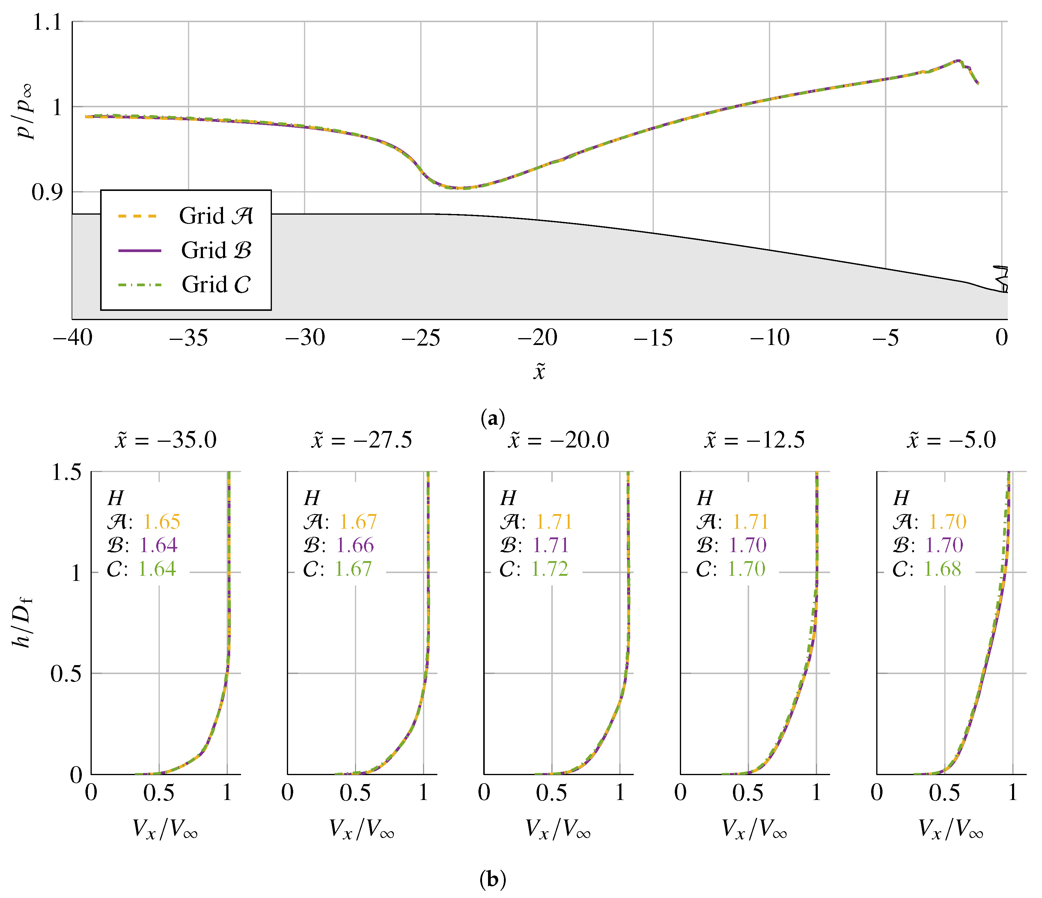
Appendix A. Grid Dependency Study

To investigate the effect of mesh resolution on the computed flow field, a grid dependency study was performed. Two grids, a selectively-refined (grid A ) and a coarsened version (grid C ) of the baseline computational grid (grid B ) for the external flow field over the BLI installation, were prepared. In the coarsened grid ( C ), the number of nodes along each dimension of the blocks were approximately halved. This leads to a grid of 11 million cells, roughly an eighth of the baseline grid, which has 87 million cells. In the selectively refined grid ( A ), the boundary layer mesh and the blocks above the fuselage ramp have been refined in the wall normal direction by a factor of 1.5 approximately, leading to a total cell count of 111 million.
Since only the discretization of the grid is of interest, the comparison among the three grids is carried out using steady RANS computations with the same solver settings and boundary conditions. The propulsor is modelled using the inlet–outlet boundaries approach, by connecting a dummy nozzle to the propulsor inlet and setting an outlet static pressure at the dummy nozzle exit. At the nozzle entry, an inlet boundary condition is imposed to model the flow exiting the stator.
Figure A1a shows the comparison of surface static pressure distribution at the centre plane across the three grids. It can be observed that the coarse grid is sufficient to resolve the pressure field. Meanwhile, the boundary layer profiles in Figure A1b show that the coarse grid, grid C , is insufficient to resolve the boundary layers, especially at the BL edge towards the end of the fuselage ramp, at x ˜ = 12.5 and 5 , whilst the profiles in grids A and B show good agreement along the ramp. Furthermore, the total dissipation rate Φ within regions A, B and C (Figure 18) of CV V for grids A and C differs from the baseline grid B by retain-explicit-plus 1.1 % and −7.8%, respectively. The results in this grid dependency study suggest that the baseline grid used in the main study is sufficient for resolving the flow features of interest and the application of the power balance method.
To assess the rate of convergence of the numerical scheme, the absolute deviations of the mass-averaged total temperature at propulsor inlet T 0 , f ¯ from the freestream value T 0 , are plotted against the relative cell size in Figure A2. As the surfaces are adiabatic and the flow does not experience any work input prior to entering the propulsor, the total temperature at propulsor inlet T 0 , f should be equal to T 0 , , the value prescribed at the domain inlet and freestream boundary, in the absence of numerical errors. The cell size h is estimated by considering the cell volume V C in the structure grid blocks leading up to the propulsor inlet above the fuselage ramp: h = [ ( V C ) / N ] 1 / 3 , where N is the cell count in those blocks. The graph shows that the error, as measured by the temperature deviations, converges with the cell size at an order of approximately 1.5, which is similar to the second-order spatial discretization scheme of the solver. Using this estimated order of convergence, the grid convergence indices for the fine and coarse grids are estimated to be 0.1% and 0.03%, respectively.
Figure A1. Flow field along the fuselage contraction at the centre plane for three different grids. (a) Surface static pressure distribution. (b) Boundary layer profiles and boundary layer shape factor H at various locations along the ramp.
Aerospace 10 00122 g0a1
Figure A2. Deviations of the mass-averaged total temperature at propulsor inlet T 0 , f ¯ from the freestream value against relative cell size h / h B .
Aerospace 10 00122 g0a2

Appendix B. Power Balance Method

The mechanical work equation can be derived by taking the dot product of V and the Navier–Stokes momentum equation:
t 1 2 ρ V 2 + · ρ V 1 2 V 2 = · ( p V ) + p · V + · ( τ ¯ ¯ · V ) ( τ ¯ ¯ · ) · V .
The above equation can be transformed to take the freestream conditions V and p into account, leading to
t 1 2 ρ ( V 2 V 2 ) + · ρ V 1 2 ( V 2 V 2 ) = · [ ( p p ) V ] + ( p p ) · V + · ( τ ¯ ¯ · V ) ( τ ¯ ¯ · ) · V .
The various types of surfaces of the control volume are defined in Section 2.2.1. Some of the volume integrals can be simplified through the divergence theorem and the boundary definitions:
· ( A )   d V = ( A ) · n ^   d S = ( A ) · n ^   d S ext + ( A ) · n ^   d S MW + ( A ) · n ^   d S FW .
Integrating Equation (A2) with respect to CV V in Figure 3 and using the Reynolds transport theorem will lead to the area and volume integral terms
d d t 1 2 ρ ( V 2 V 2 ) d V   d E   d t 1 2 ρ ( V 2 V 2 ) V MW · n ^   d S MW + ( p p ) + 1 2 ρ ( V 2 V 2 ) V τ ¯ ¯ · V · n ^   d S = ( p p ) · V   d V P V ( τ ¯ ¯ · ) · V   d V Φ .
The above equation contains three volume integrals. The first, d E /   d t , tracks the changes in mechanical energy within V with time, and will be negligible if the flow field is steady or periodic-unsteady upon time-averaging. The second volume integral is the net pressure-volume power P V , whilst the final term is the viscous dissipation rate Φ , with the local rate of dissipation per unit volume given by ϕ = ( τ ¯ ¯ · ) · V . With the RANS approach under the Boussinesq assumption, ϕ = ( τ ¯ ¯ eff · ) · V , where τ ¯ ¯ eff = ( μ + μ t ) [ V + ( V ) T ] is the effective shear stress, i.e., sum of viscous and turbulent shear stresses. Therefore,
Φ = ( τ ¯ ¯ · ) · V ϕ   d V = ( τ ¯ ¯ eff · ) · V   d V .
This is similar to the approach in Sanders and Laskaridis [36]. The closed surface integrals can be split into contributions from the various boundaries using Equation (A3), and noting V = 0 on S FW and V = V MW on S MW :
d E d t + Φ + ( p p ) + 1 2 ρ ( V 2 V 2 ) V τ ¯ ¯ · V · n ^   d S ext = ( p p ) V + τ ¯ ¯ · V · n ^   d S MW + P V .
As the propulsor internal domain is included in the CV V used in this study, as depicted in Figure 3, its power input is accounted for through the moving surfaces in the shaft power P S term:
P S = ( p p ) V + τ ¯ ¯ · V · n ^   d S MW .
Moreover, Φ and P V also include contributions from the propulsor internal domain.
The power balance then becomes
P S + P V = d E d t + E ˙ + Φ ,
where E ˙ is the mechanical energy outflow rate at the external boundaries S ext :
E ˙ = ( p p ) V + 1 2 ρ ( V 2 V 2 ) V τ ¯ ¯ · V · n ^   d S ext .
To aid understanding, the outflow rate can be decomposed into contributions from the individual external surfaces:
E ˙ = V · F + all S ext ( E ˙ u + E ˙ p + E ˙ τ ) E ˙ ,
where F is the far-field force acting on the aircraft portion surrounded by the CV by considering the fluxes on the external boundaries. E ˙ u is the wake/jet kinetic energy deposition rate, and E ˙ p is the pressure work deposition rate. E ˙ τ is the viscous stress work deposition rate.
F = ( p p ) n ^ + ( V V ) ( ρ V · n ^ ) τ ¯ ¯ · n ^   d S ext
E ˙ u = 1 2 ρ | V V | 2 V · n ^   d S
E ˙ p = ( p p ) ( V V ) · n ^   d S
E ˙ τ = τ ¯ ¯ · ( V V ) · n ^   d S
The terms shaded in Equations (1), (2), (A10) and (A11) represent viscous stress contributions on the propulsor inflow/outflow and external boundaries. In practice, they are usually negligible at the propulsor inlets, outlets and external boundaries, except in the case when the control volume is a captured streamtube, which is fully submerged within the boundary layer.

References

  1. Tse, T.S.; Hall, C.A. Flow Field and Power Balance of a Distributed Aft-fuselage Boundary Layer Ingesting Aircraft. In Proceedings of the AIAA Propulsion and Energy 2020 Forum, Virtual Event, 24–28 August 2020. [Google Scholar] [CrossRef]
  2. Hileman, J.I.; Spakovszky, Z.S.; Drela, M.; Sargeant, M.A.; Jones, A. Airframe Design for Silent Fuel-Efficient Aircraft. J. Aircr. 2010, 47, 956–969. [Google Scholar] [CrossRef] [Green Version]
  3. Drela, M. Development of the D8 Transport Configuration. In Proceedings of the 29th AIAA Applied Aerodynamics Conference, Honolulu, HI, USA, 27–30 June 2011. [Google Scholar] [CrossRef]
  4. Welstead, J.; Felder, J.L. Conceptual Design of a Single-Aisle Turboelectric Commercial Transport with Fuselage Boundary Layer Ingestion. In Proceedings of the 54th AIAA Aerospace Sciences Meeting, San Diego, CA, USA, 4–8 January 2016. [Google Scholar] [CrossRef] [Green Version]
  5. Seitz, A.; Habermann, A.L.; Peter, F.; Troeltsch, F.; Castillo Pardo, A.; Della Corte, B.; van Sluis, M.; Goraj, Z.; Kowalski, M.; Zhao, X.; et al. Proof of Concept Study for Fuselage Boundary Layer Ingesting Propulsion. Aerospace 2021, 8, 16. [Google Scholar] [CrossRef]
  6. Seitz, A.; Gologan, C. Parametric design studies for propulsive fuselage aircraft concepts. CEAS Aeronaut. J. 2015, 6, 69–82. [Google Scholar] [CrossRef]
  7. Steiner, H.J.; Seitz, A.; Wieczorek, K.; Plötner, K.; Isikveren, A.T.; Hornung, M. Multi-disciplinary design and feasibility study of distributed propulsion systems. In Proceedings of the 28th International Congress of the Aeronautical Sciences (ICAS), Brisbane, Australia, 23–28 September 2012. [Google Scholar]
  8. National Academies of Sciences, Engineering, and Medicine. Commercial Aircraft Propulsion and Energy Systems Research; The National Academies Press: Washington, DC, USA, 2016. [Google Scholar] [CrossRef]
  9. Cumpsty, N.; Heyes, A. Jet Propulsion, 3rd ed.; Cambridge University Press: Cambridge, UK, 2015. [Google Scholar] [CrossRef]
  10. Epstein, A.H.; O’Flarity, S.M. Considerations for Reducing Aviation’s CO2 with Aircraft Electric Propulsion. J. Propuls. Power 2019, 35, 572–582. [Google Scholar] [CrossRef]
  11. Jansen, R.H.; Celestina, M.L.; Kim, H.D. Electrical Propulsive Fuselage Concept for Transonic Transport Aircraft. In Proceedings of the 24th ISABE Conference, Canberra, Australia, 22–27 September 2019. [Google Scholar]
  12. Plas, A.P.; Sargeant, M.A.; Madani, V.; Crichton, D.; Greitzer, E.M.; Hynes, T.P.; Hall, C.A. Performance of a Boundary Layer Ingesting (BLI) propulsion system. In Proceedings of the 45th AIAA Aerospace Sciences Meeting and Exhibit, Reno, NV, USA, 8–11 January 2007; Volume 8, pp. 5368–5388. [Google Scholar] [CrossRef] [Green Version]
  13. Gunn, E.J.; Hall, C.A. Aerodynamics of Boundary Layer Ingesting Fans. In Proceedings of the ASME Turbo Expo 2014: Turbine Technical Conference and Exposition, Düsseldorf, Germany, 16–20 June 2014;A; Volume 1A, p. V01AT01A024. [Google Scholar] [CrossRef]
  14. Gunn, E. Aerodynamics of Boundary Layer Ingesting Fans. Ph.D. Thesis, University of Cambridge, Cambridge, UK, 2015. [Google Scholar]
  15. Giesecke, D.; Friedrichs, J. Aerodynamic Comparison Between Circumferential and Wing-Embedded Inlet Distortion for an Ultra-High Bypass Ratio Fan Stage. In Proceedings of the ASME Turbo Expo 2019: Turbomachinery Technical Conference and Exposition, Phoenix, AZ, USA, 17–21 July 2019. [Google Scholar] [CrossRef]
  16. Drela, M. Power Balance in Aerodynamic Flows. AIAA J. 2009, 47, 1761–1771. [Google Scholar] [CrossRef] [Green Version]
  17. Brandvik, T.; Pullan, G. An Accelerated 3D Navier–Stokes Solver for Flows in Turbomachines. J. Turbomach. 2011, 133, 021025. [Google Scholar] [CrossRef]
  18. Spalart, P.R.; Allmaras, S.R. A One-Equation Turbulence Model for Aerodynamic Flows. La Recherche Aérospatiale 1994, 5–21. [Google Scholar]
  19. Liu, Y.; Lu, L.; Fang, L.; Gao, F. Modification of Spalart–Allmaras Model with Consideration of Turbulence Energy Backscatter Using Velocity Helicity. Phys. Lett. A 2011, 375, 2377–2381. [Google Scholar] [CrossRef]
  20. Vassberg, J.C.; Tinoco, E.N.; Mani, M.; Rider, B.; Zickuhr, T.; Levy, D.W.; Brodersen, O.P.; Eisfeld, B.; Crippa, S.; Wahls, R.A.; et al. Summary of the Fourth AIAA Computational Fluid Dynamics Drag Prediction Workshop. J. Aircr. 2014, 51, 1070–1089. [Google Scholar] [CrossRef]
  21. Tinoco, E.N.; Brodersen, O.P.; Keye, S.; Laflin, K.R.; Feltrop, E.; Vassberg, J.C.; Mani, M.; Rider, B.; Wahls, R.A.; Morrison, J.H.; et al. Summary Data from the Sixth AIAA CFD Drag Prediction Workshop: CRM Cases. J. Aircr. 2018, 55, 1352–1379. [Google Scholar] [CrossRef] [Green Version]
  22. Masaki, A.; Ogushi, S.; Tsuruta, R.; Nishiwaki, D.; Sato, T.; Okai, K.; Kazawa, J.; Masaki, D.; Harada, M. Assessment of the Influence of Boundary Layer Ingestion (BLI) on the Axial Fan. J. Phys. Conf. Ser. 2021, 1909, 012081. [Google Scholar] [CrossRef]
  23. Jerez Fidalgo, V. Fan-Distortion Interaction in Novel Aircraft Installations. Ph.D. Thesis, University of Cambridge, Cambridge, UK, 2012. [Google Scholar]
  24. Jameson, A. Time Dependent Calculations Using Multigrid, with Applications to Unsteady Flows Past Airfoils and Wings. In Proceedings of the 10th Computational Fluid Dynamics Conference, Honolulu, HI, USA, 24–26 June 1991; p. 1596. [Google Scholar] [CrossRef]
  25. Ayachit, U. The ParaView Guide; Kitware Inc.: Clifton Park, NY, USA, 2019; Updated for ParaView version 5.6. [Google Scholar]
  26. Pandya, S.A.; Uranga, A.; Espitia, A.; Huang, A. Computational Assessment of the Boundary Layer Ingesting Nacelle Design of the D8 Aircraft. In Proceedings of the 52nd Aerospace Sciences Meeting, National Harbor, MD, USA, 13–17 January 2014. [Google Scholar] [CrossRef]
  27. Maldonado, Y.B.; Giannakakis, P.; Rodriguez, B.; Tantot, N. Book-keeping investigations for BLI aircraft. In Proceedings of the AIAA Propulsion and Energy 2020 Forum, Virtual Event, 24–28 August 2020. [Google Scholar] [CrossRef]
  28. Vassberg, J.C.; DeHaan, M.A.; Rivers, M.S.; Wahls, R.A. Retrospective on the Common Research Model for Computational Fluid Dynamics Validation Studies. J. Aircr. 2018, 55, 1325–1337. [Google Scholar] [CrossRef]
  29. Korsia, J.J.; De Spiegeleer, G. VITAL, An European R&D Program for Greener Aero-engines. In Proceedings of the 25th International Congress of the Aeronautical Sciences, Hamburg, Germany, 3–8 September 2006. [Google Scholar]
  30. Spalart, P.R.; Rumsey, C.L. Effective Inflow Conditions for Turbulence Models in Aerodynamic Calculations. AIAA J. 2007, 45, 2544–2553. [Google Scholar] [CrossRef]
  31. Jerez Fidalgo, V.; Hall, C.A.; Colin, Y. A Study of Fan-Distortion Interaction Within the NASA Rotor 67 Transonic Stage. J. Turbomach. 2012, 134, 051011. [Google Scholar] [CrossRef]
  32. Heinlein, G.; Chen, J.; Bakhle, M. Aerodynamic Behavior of a Coupled Boundary Layer Ingesting Inlet – Distortion Tolerant Fan. In Proceedings of the AIAA Propulsion and Energy 2020 Forum, Virtual Event, 24–28 August 2020. [Google Scholar] [CrossRef]
  33. Castillo Pardo, A.; Mehdi, A.; Pachidis, V.; MacManus, D.G. Numerical Study of the Effect of Multiple Tightly-Wound Vortices on a Transonic Fan Stage Performance. In Proceedings of the ASME Turbo Expo 2014, Düsseldorf, Germany, 16–20 June 2014; Volume 1A, p. V01AT01A033. [Google Scholar] [CrossRef]
  34. Tucker, P.G. Trends in turbomachinery turbulence treatments. Prog. Aerosp. Sci. 2013, 63, 1–32. [Google Scholar] [CrossRef]
  35. Hue, D.; Chanzy, Q.; Landier, S. DPW-6: Drag Analyses and Increments Using Different Geometries of the Common Research Model Airliner. J. Aircr. 2018, 55, 1509–1521. [Google Scholar] [CrossRef]
  36. Sanders, D.S.; Laskaridis, P. Full-Aircraft Energy-Based Force Decomposition Applied to Boundary-Layer Ingestion. AIAA J. 2020, 58, 4357–4373. [Google Scholar] [CrossRef]
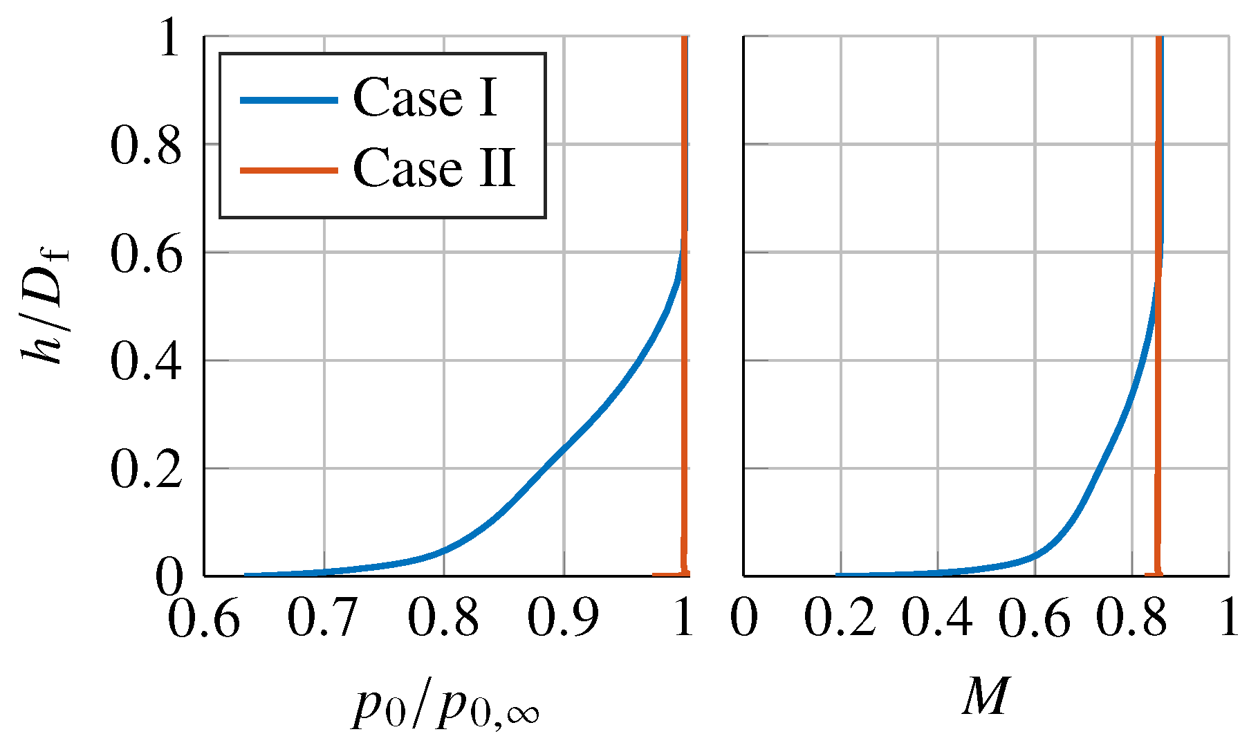
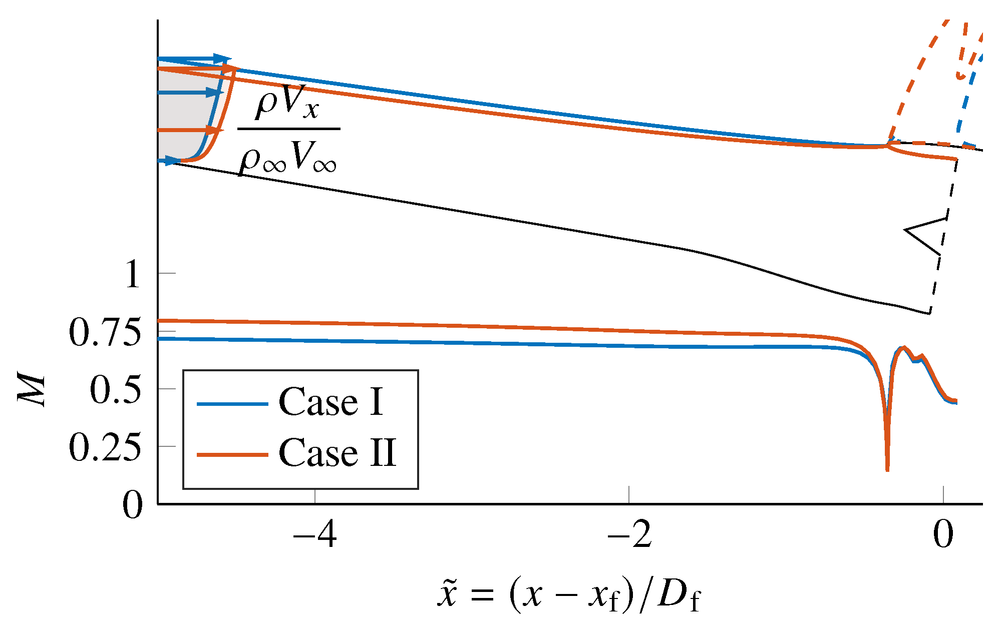
Figure 1. Distributed aft-fuselage BLI aircraft concept.
Aerospace 10 00122 g001
Figure 2. Computational domain and boundary conditions.
Aerospace 10 00122 g002
Figure 3. Control volume V for mechanical power balance. The external surface S ext is in red, moving surfaces S MW in orange, stationary viscous walls S FW in black, and the propulsor inlet and outlet S IO , prop are in blue.
Aerospace 10 00122 g003
Figure 4. Details of the installation. (a) 3D view. (b) Propulsor meridional view showing the two different nozzle plugs for cases I and II.
Aerospace 10 00122 g004
Figure 5. Profiles of stagnation pressure p 0 and Mach number M at CFD domain inlet ( x ˜ = 39.8 ), centre plane.
Aerospace 10 00122 g005
Figure 6. Mach number M at centre plane, with M = 1 contour in yellow. (a) Case I. (b) Case II.
Aerospace 10 00122 g006
Figure 7. Boundary layer profiles: variations of V x / V with distance from surface h / D f . Horizontal dashed lines mark δ / D f the BL extent by stagnation pressure p 0 = 0.998 p 0 , .
Aerospace 10 00122 g007
Figure 8. Cowl surface isentropic Mach number M isen .
Aerospace 10 00122 g008
Figure 9. Stagnation streamline at centre plane and its variations of Mach number M. The M = 1 contours are in dashed lines and the profiles of mass flux ( ρ V x ) / ( ρ V ) at x ˜ = 5 are shaded.
Aerospace 10 00122 g009
Figure 10. Top view showing surface static pressure p / p and the streamlines over the cowl. (a) Case I. (b) Case II.
Aerospace 10 00122 g010
Figure 11. Reversed flow extent, indicated by the V x = 0 isolines, near nozzle exit, location as indicated in Figure 12. The high dissipation regions are shaded in colour, with case I overlaid onto case II. The exhaust geometry is in grey, with the different plug profiles: case I Aerospace 10 00122 i003, and case II Aerospace 10 00122 i004.
Aerospace 10 00122 g011
Figure 12. Exhaust jet velocity profiles at the centre plane. The streamlines showing the extent of the exhaust jet are in dotted lines. The regions of p / p 1.2 are shaded, with the case I region overlaid onto case II. The orange line (Aerospace 10 00122 i001
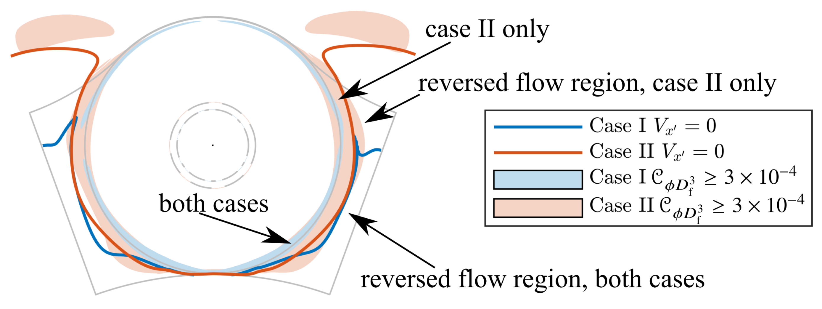
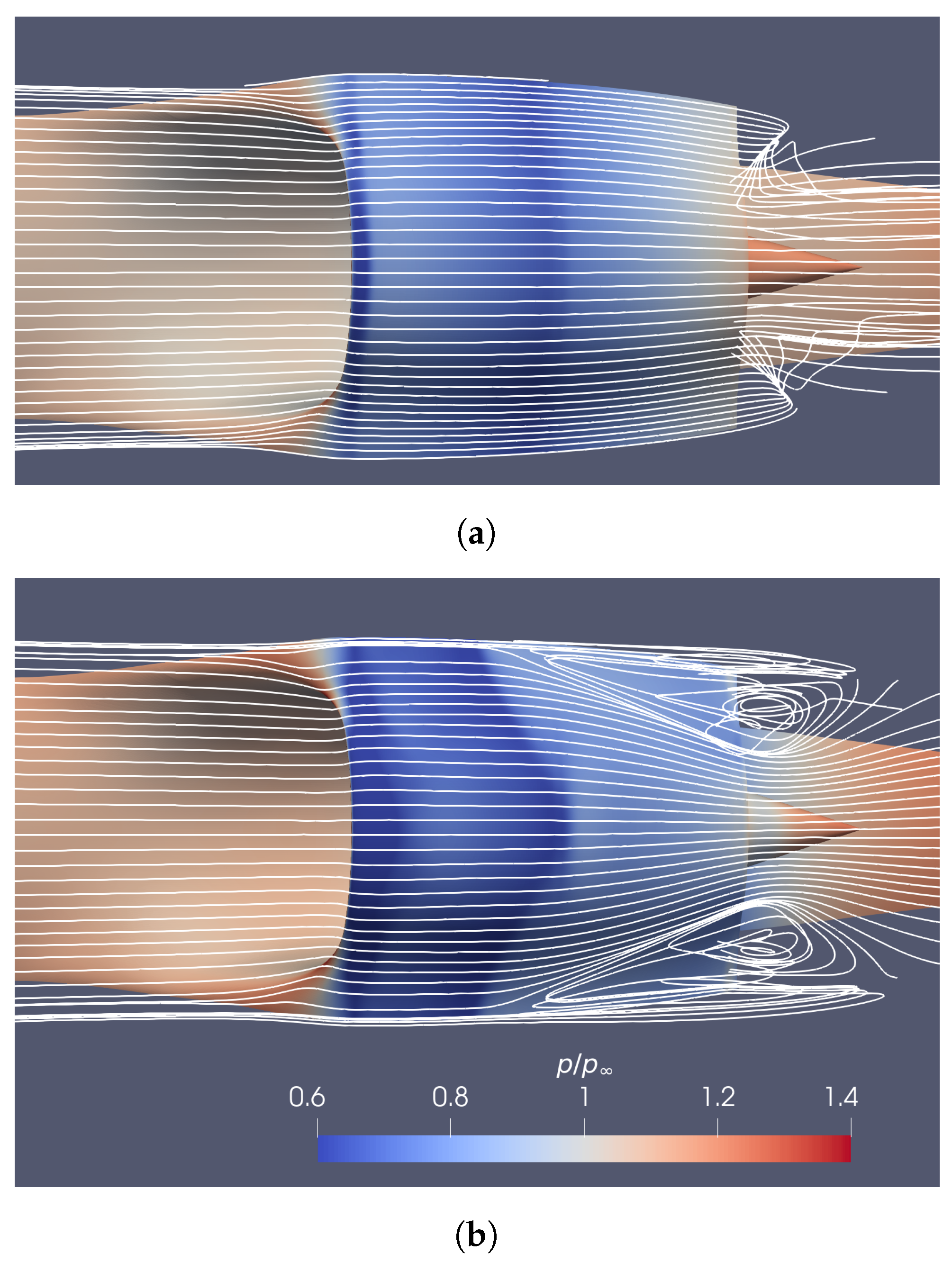
) denotes the cut plane for Figure 11.
Aerospace 10 00122 g012
Figure 13. Fan characteristics showing variations of total–total pressure ratio r p and total–total isentropic efficiency η tt with normalised mass flow rate Q f through the propulsor at the design normalised fan rotational speed N Ω .
Aerospace 10 00122 g013
Figure 14. Propulsor inlet distortion, case I. (a) Total pressure distribution p 0 / p 0 , . (b) Turbulent viscosity ratio μ t / μ .
Aerospace 10 00122 g014
Figure 15. Entropy function relative to the freestream ζ = exp [ ( s s ) / R ] at the rotor downstream (plane RW in Figure 16) from the instantaneous flow field. (a) 50% span. (b) 75% span.
Aerospace 10 00122 g015
Figure 16. Instantaneous propulsor blade-to-blade variations of Mach number in the local reference frame near tip, 90% rotor span, for case I. The Mach 1 line is in orange.
Aerospace 10 00122 g016
Figure 17. Circumferential variations of changes in the incidence angle relative to operation in the uniform flow at the propulsor inlet at various span fractions. Flow stagnates on the blade pressure surface with a positive incidence angle i.
Aerospace 10 00122 g017
Figure 18. Mechanical power balances for CV V , full 360° fuselage. The dissipation rates Φ have been broken down into the contributions from the four regions in the inset.
Aerospace 10 00122 g018
Table 1. Operating conditions.
ParameterValue
Cruise altitude12 km (FL394)
M 0.85
p 1.93 × 10 4 Pa
T 216.7 K
μ 1.42 × 10 5 N s m−2
c p 1005 J kg−1 K−1 s
γ 1.4
P r 1
ν ˜ 5 μ / ρ [30]
Table 2. Test case parameters. δ * is the BL displacement thickness.
Test CaseInlet Profile A N / A N , I δ * ( x ˜ = 5 ) / D f Intake Flow Ratio A / A t
Case I (BLI)Realistic BL profile1.000.2240.637
Case II (Thin BL)Uniform p 0 0.950.1170.687
Disclaimer/Publisher’s Note: The statements, opinions and data contained in all publications are solely those of the individual author(s) and contributor(s) and not of MDPI and/or the editor(s). MDPI and/or the editor(s) disclaim responsibility for any injury to people or property resulting from any ideas, methods, instructions or products referred to in the content.

