Abstract
An aeroservoelastic system can be described as a gridding-based linear parameter-varying (LPV) model, whose dynamic characteristics usually vary with the airspeed. Due to the high order of the system, it is necessary to perform order reduction on LPV models to overcome the control design challenges. However, when directly extending linear time-invariant (LTI) model order reduction technologies to the LPV system, states of the reduced-order LTI models generated separately at different grid points could be inconsistent. In this paper, a novel modal matching algorithm is proposed to solve the problem of state inconsistency by identifying the internal connection between the models at adjacent grid points. An oblique projection-based distance metric is defined to improve the reliability of the modal matching algorithm. The reduced-order LPV model constructed based on this method would have a high fidelity relative to the original model and a smooth interpolation performance between grid points. The proposed algorithm is applied to the X-56A aircraft, and numerical results show its effectiveness.
1. Introduction
In recent years, extensive research has been conducted on the modeling and control of rigid-flexible coupling aircraft, such as the X-56 Multi-Utility Technology Testbed (MUTT) aircraft designed by Lockheed Martin [1,2,3,4,5,6]. The typical issue with this flexible flying-wing aircraft is the body-freedom flutter (BFF) phenomenon [7,8]. It has a strong coupling between structural vibration and rigid body motion, which is quite different from the flutter of two-dimensional airfoils or three-dimensional wings [9,10]. The nonlinear model that describes the X-56A consists of rigid body dynamics, structural dynamics, unsteady aerodynamics, actuator models, and sensor models, leading to a high-dimensional system [11]. Even though the structural modes and aerodynamic lag states that are insignificant and negligible have been truncated and residualized, the order of the X-56A aeroservoelastic model is still in the hundreds, posing challenges for control design. The European Flutter Free FLight Envelope eXpansion for ecOnomical Performance improvement (FLEXOP) project developed a similar flutter demonstrator, which is also modeled as a high-order aeroservoleastic system and faces control design challenges [12,13].
It is noticed that aeroservoelastic characteristics vary with the airspeed. Therefore, nonlinear models of flexible aircraft can be approximated as a gridding-based linear parameter-varying (LPV) model [14], which consists of a family of state-space representations linearized at different airspeeds (i.e., grid points or operating points). However, for most flutter control schemes, a controller is usually first designed at a chosen grid point and then verified at other grid points [15,16,17,18,19]. The single-point design method is not only a tedious process, it also cannot guarantee performance and even stability when the airspeed varies between grid points. By solving a linear-matrix-inequality-based optimization problem, an LPV controller can be designed by considering all grid points, and the controller gain can be automatically scheduled with the airspeed [20,21]. However, this may lead to high computational costs when applying the LPV control method to complex aeroservoelastic systems (e.g., those with more than 50 state variables) [14,22]. A reliable low-dimensional approximate model is needed for the controller design of the flexible aircraft.
The model order reduction process of LPV systems [3] can be implemented step-by-step according to four linear time-invariant (LTI) technologies: truncation, residualization, modal decomposition [4], and balanced truncation [23]. The technologies of the last two steps are used to achieve the final objective by finding an appropriate transformation function to map the high-dimensional state vector to a lower-dimensional state space , where denotes the real space and . Note that the state-space expression of a specific LTI system is not uniquely defined. It can be transformed from one state space to another by an invertible state transformation matrix. When those LTI technologies are directly extended to LPV models, local transformations are generated independently at grid points. The resulting local state variables or their ordering may be different at different grid points. This problem is called state inconsistency [24,25].
The internal relationship between local models should be identified in order to construct consistent transformations [24]. The modal matching method is proposed to address the state inconsistency problem encountered in the modal-decomposition-based model reduction technique [4]. This method is also needed in the process of flutter prediction to keep the correct mode tracking between airspeed steps [26].
The implementation of the existing modal matching method mentioned above consists of two steps [27,28,29]. Firstly, a metric function is constructed to compute the distance between the eigenvalues of adjacent local models. Then, a decision criterion is defined to match the eigenvalues and corresponding eigenvectors according to the distance. For example, a hyperbolic distance metric is adopted and the Kuhn–Munkres algorithm is chosen to find a perfect matching in a bipartite graph [29]. To make the distance metric reliable enough, a weighted distance metric is proposed in that method by considering the associated eigenvectors in addition to the information on the eigenvalues. However, for eigenvalues with a multiplicity greater than 1, the corresponding eigenvectors are not uniquely determined by eigendecomposition. These eigenvectors should be detected and determined first before calculating the distance [29].
This paper proposes a new distance metric generated using the oblique projection matrices [30]. The distance metric consists of a Kronecker delta and a perturbed term. The delta term makes it easy to identify the paired oblique projection matrices and thus simplify the modal matching process. In addition, the proposed oblique-projection-based modal matching algorithm can handle the special cases of multiple eigenvalues (e.g., repeated roots and complex–real transitions) without taking complex measures such as the Procrustes smoothing method used in [29].
The rest of this paper is organized as follows. The state inconsistency problem encountered in the process of LPV model order reduction is introduced in Section 2. Then, Section 3 gives the background knowledge of the oblique projection, based on which a new distance metric is defined between local grid points. In addition, a method to rematch the eigenvalues and to deal with the extremely closed eigenvalue trajectories is also proposed. In Section 4, the proposed algorithm is applied to obtain the LPV reduced-order model of the X-56A flexible aircraft. Finally, Section 5 concludes the paper.
2. Problem Formulation
This section starts with the introduction of the gridding-based LPV model for the X-56A aircraft. The basic concept of the projection-based LPV model order reduction technology is then described, especially for the modal decomposition method. The state-inconsistent problems that the current modal matching algorithm cannot effectively deal with are discussed in detail.
2.1. Model of the Aeroservoelastic System
NASA’s X-56A MUTT is an experimental flying-wing aircraft for the study of BFF suppression [31]. Figure 1 shows the schematic of the X-56A with a wingspan of 4.27 m. The first 8 structural elastic modes of the aircraft are listed in Table 1. Based on numerical calculations, the BFF phenomenon arises when the flying-wing aircraft reaches its critical flutter airspeed of about 68 m/s. This phenomenon behaves as a coupling of the short-period mode of the flight dynamics and the first symmetric elastic mode of the structural dynamics. The 7 other elastic modes listed in Table 1 provide less significant contributions to the BFF phenomenon, but they are also recorded to establish the high-fidelity aeroservoelastic model.
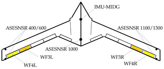
Figure 1.
Schematic of X-56A MUTT.

Table 1.
Structural Free-Vibration Characteristics.
For the active suppression of the BFF phenomenon, the outer flaps are allocated as control inputs, denoted as and . As shown in Figure 1, the former denotes the symmetric deflection of the flaps WF3L and WF3R, and the latter corresponds to the symmetric deflection of the flaps WF4L and WF4R. There are 3 measurement outputs. The pitch rate is measured by an IMU-MIDG gyroscope, the acceleration at the center body is measured by an ASESNSR 1000 accelerometer, and is a processed integrated signal measured by four wingtip accelerometers, ASESNSR 400, 600, 1100, 1300.
The open-source model [28] has been simplified by the truncation and residualization of negligible lateral states and high-frequency structural modes. It is a gridding-based LPV model developed for controller design, and the airspeed is chosen as the scheduling parameter ranging from 30.6 m/s to 68 m/s. Within this range, 12 different values of the airspeed are selected, and the state-space representation of the aeroservoelastic system at each airspeed is obtained. These 12 different airspeeds are considered grid points, and the resulting 12 state-space models form a gridding-based LPV model given by the pair .
where , , and are the state, input, and output vectors, respectively. , , , and are the constant matrices obtained at the scheduling parameter , where the subscript k denotes the k-th grid point. The state vector of the LPV model consists of 2 rigid body states (the angle of attack and the pitch rate q), 8 structural modes (generalized coordinates and , where each is an 8 × 1 vector), and 30 aerodynamic states (w, a 30 × 1 vector), resulting in a total of 48 state variables. Because the order of the model is still too high and not simple enough for control design, it is necessary to perform model order reduction before control synthesis.
2.2. Projection-Based LPV Model Order Reduction
Consider an LPV model in the general form
For controller synthesis, a low-order model is desired to approximate a high-dimensional LPV model. Different projection-based LPV model order reduction methods are proposed to solve this problem, and they can be generalized as the following two steps [32].
(1) Generate a state transformation matrix function such that . The original LPV model (2) can be rewritten as
where z can be divided into two parts, i.e., . Correspondingly, is partitioned as , and its inverse is .
(2) Truncate the vector that makes a negligible contribution to the output response. The reduced-order model is then formulated as
Then, the gridding-based reduced-order model at can be expressed as
From the engineering application perspective, it should be pointed out that the LPV model of an aeroservoelastic system is usually expressed in the form of Equation (1) instead of Equation (2). LTI technologies can be applied to obtain a reduced-order model at each grid point. However, the local transformation matrices and would not be uniquely expressed because they could vary with an invertible state transformation matrix. States of the reduced-order LTI models may be inconsistent, and thus the reduced-order LTI models cannot be simply grouped together as a gridding-based LPV model for LPV control synthesis. To solve this issue, this paper focuses on the modal matching method to generate the desired consistent transformations and using the local matrices and . Details of the proposed method will be given in Section 3.
2.3. Eigendecomposition of a Matrix-Valued Function
Consider the state matrix function in Equation (2). The matrix-valued function is assumed to be diagonalizable, and the case of algebraic multiplicity is considered in the following discussion. Its eigendecomposition is given as
where denotes the eigenvalue function and denotes the corresponding eigenvector function. The method to generate for Equation (3) using the above Equation (6) is called modal decomposition. Note that eigenvalues and eigenvectors vary with the scheduling parameter . The eigenvalue trajectories and corresponding eigenvectors are proved to have analytic expressions if multiplicities of the eigenvalues are 1 in the whole parameter range [33]. If multiplicities are greater than 1, it has been proven that analytic expressions also exist when additional conditions are satisfied [34]. The inverse of is written as . Then, the matrix-valued function can be expressed as
Similarly, for the gridding-based LPV model, the eigendecomposition is computed individually at each local grid point .
where the subscript i denotes the i-th eigenvalue or eigenvector. Because the eigenvalues in Equation (8) are usually rearranged from large to small according to their magnitudes, the corresponding sequence may not be equal to that from Equation (7).
Even if the eigenvalues are paired, i.e., the left and right sides of Equation (9) are equal, the corresponding eigenvectors may not be equal to each other because the eigenvectors of a matrix are not unique.
To make the eigenvectors continuously vary between grid points, the eigenvector is scaled by a scalar l.
Thus, the normalized eigenvectors can be smoothly interpolated between grid points. However, this introduces additional constraints by letting and will reduce the solvable region of the transformation .
2.4. Modal Matching Algorithm
To help the reader easily understand the modal matching algorithm, the poles (which are also the eigenvalues of the state matrix) of the X-56A aeroservoelastic system are shown in Figure 2. The poles migrate when the airspeed varies and create trajectories in the complex plane. A modal matching algorithm is a systematic approach to pairing the eigenvalues and eigenvectors. When the scheduling parameter varies from to , it can automatically find the migration of each eigenvalue, and the same is true for the corresponding eigenvector.
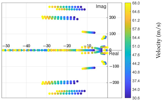
Figure 2.
Pole migration of the X-56A model when the velocity varies from 30.6 m/s to 68.0 m/s.
As shown in Figure 3, the i-th eigenvalue trajectory and the corresponding information and are defined as subset i. During the matching process, a structure array is used to record the data in a subset, which is updated at each step by appending the paired eigenvalues. The algorithm starts from the first grid point where the i-th eigenvalue is labeled as and assigned to subset i. Then, the eigenvalue at the next grid point is detected, paired, and recorded in the subset (labeled as ). The second step is repeated point-by-point. The elements in subset i eventually form the eigenvalue trajectory , where is the number of grid points. The corresponding eigenvector trajectory is also recorded to generate the desired consistent transformations , where .
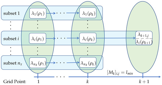
Figure 3.
Put the paired eigenvalue into subset i and form the i-th eigenvalue trajectory .
The above steps depend on a metric function to measure the distance between the eigenvalues of the neighboring grid points k and . There are different definitions for this function. For example, eigenvectors are also considered to increase the reliability of the metric [29], which can be expressed as a function of both eigenvalues and eigenvectors at neighboring grid points (see Equation (12)). The paired eigenvalue is identified if it has the minimum distance compared to other eigenvalues at grid point .
The existing matching algorithm is based on the assumption of a one-to-one correspondence for eigenvalue trajectories. However, as shown in Figure 4, if eigenvalues and are identical, Equation (12) will give the same distance values, and it is not clear which eigenvalue should be paired.
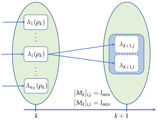
Figure 4.
Multiple eigenvalues exist when pairing the eigenvalues.
Cases with multiple eigenvalues can be classified into two categories.
(1) Repeated trajectories. Such special cases are encountered in aeroservoelastic systems. Take the X-56A model given in Section 2.1 as an example. There are 10 identical eigenvalues to describe the dynamics of control flaps when the same actuators are used. Those eigenvalues and related eigenvectors cannot be paired individually by the eigendecomposition alone.
(2) Crossing trajectories. When two eigenvalue trajectories intersect, the multiplicity is 2 at the intersection point. The complex–real transformation is a special case, in which the intersection happens when two conjugate poles meet on the real axis and the damping ratio varies from underdamped to critically damped and overdamped.
In both cases, there are extremely close eigenvalue trajectories, which can be explained and visualized using simple examples. As shown in Figure 5, multiple eigenvalues at intersections would have the same least distance relative to the adjacent eigenvalue, and eigenvectors must be considered in the distance metric to provide more information. However, as given in Equation (13), the corresponding eigenvectors can be arbitrarily transformed by an invertible matrix X, and these eigenvectors should be uniquely determined first.
where . However, it is not easy to obtain a matrix X that can make the eigenvector trajectories vary smoothly with grid points. Therefore, it is worth improving the modal matching algorithm and finding a high-quality LPV model order reduction method.
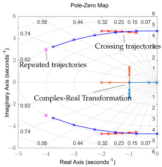
Figure 5.
Examples of multiple eigenvalues, e.g., repeated roots, the crossing trajectories, and the complex-real transformation.
3. Oblique-Projection-Based Modal Matching Algorithm
A new type of distance metric is defined in Section 3.1 based on the concept of oblique projection. As shown in Section 3.2, special trajectories may be found to belong to multiple subsets, not one-to-one correspondences. Thus, they are merged into one subset for further processing. As given in Section 3.3, a newly proposed method is applied to reconstruct the consistent transformations . The implementation procedure of the algorithm is summarized in Section 3.4.
3.1. Definition of an Oblique-Projection-Based Distance Metric
For a vector space , if the subspace and its complementary subspace satisfy the condition that and , the projection is called the oblique projection on along . It can be parameterized by a constant matrix and a symmetric positive definite matrix . The oblique projection is uniquely characterized by the basis subspace spanned by V and the test subspace spanned by , as written in Equation (14).
Details about the properties of the oblique projection are given in [30]. It is shown that a matrix is an oblique projection if and only if it is idempotent.
As described in Equation (7), is exactly a continuous oblique projection function, which can be proved by the orthogonal condition .
The oblique projection matrix is uniquely determined according to its definition no matter what size the eigenvector described in Equation (11) is scaled to. Furthermore, the matrix at the local grid point has more information than the scalar , and thus, it can be a good candidate for the definition of the metric function, as shown in Figure 6.

Figure 6.
Putting the paired oblique projection matrix into subset i and forming the i-th oblique projection sequence .
In this paper, the oblique projection matrix is used instead of eigenvalues to construct a new distance metric function. Consider the relationship between two oblique projection matrices and at the local grid point k.
The above equation is derived by the orthogonal condition . It indicates that the oblique projection matrix has the “orthogonal characteristic”, and the distance between the adjacent grid points can also be evaluated by this property.
Suppose that could be expressed as a paired matrix plus perturbed terms.
where and indicate the error caused by a step length . The orthogonal condition is considered such that , and thus,
Then, the relationship between two oblique projection matrices and is evaluated by calculating .
where
The above equation is obtained by considering the orthogonal condition . Note that the second term and the third term exist only when , and thus, Equation (19) is adopted to replace two terms.
Finally, Equation (20) can be simplified as
The perturbation is a second-order small quantity if the step size is small enough, and thus, the distance is mainly determined by . A new metric function is defined by using this type of method to evaluate the distance of oblique projection matrices between the grid points k and .
where the -norm is adopted to calculate the matrix norm in the above equation to obtain the scalar distance.
The decision criterion for the proposed matching algorithm is much easier compared to seeking the minimum distance of in Section 2.4: two oblique projection matrices are paired if the Kronecker delta equals 1 and unpaired if equals 0. To consider the effect of the perturbed term, a tolerance value is included in the decision criterion, as given in Equation (24).
This indicates that the step size is too large (i.e., the grid points are not dense enough) when almost all perturbed terms in the metric are greater than the tolerance value . This problem can be addressed by increasing the density of gridding points.
3.2. Merging of the Detected Special Oblique Projection Sequences
The proposed distance metric can be used to easily identify the paired oblique projections in the matching process, except for the multiple eigenvalue cases discussed in Equation (13). Similar to the eigenvectors, the corresponding oblique projections are not uniquely determined in those special cases. Thus, if the perturbed term still exceeds the tolerance after many attempts to make the operating points denser, there may exist special cases of multiple eigenvalues.
To avoid this trial and error method, this paper proposes a new method, which is inspired by the oblique projection matrix discussed in Section 3.1. Given two eigenvalue trajectories, the corresponding eigenvectors are arbitrarily transformed by X. The sum of their oblique projection operators is expressed in Equation (26).
The above equation indicates that the sum of two oblique projection matrices is still uniquely characterized by the basis subspace and the test subspace , no matter what transformation matrix X is selected. This is true for all oblique projection matrix sequences, including special cases with multiple eigenvalues as given in Equation (13).
Take the special subsets i and j as an example. Based on the previous discussion, there is no need to distinguish which subset and should belong to. As shown in Figure 7, subsets i and j could be merged into subset , where oblique projection matrices and are added and replaced by the resulting matrix . Note that the index number of the new subset inherits from one of the original index numbers, and the hat symbol is used to distinguish them from unmerged subsets. Except for special cases with multiple eigenvalues, subsets that have complex conjugate eigenvalue trajectories are also merged into a new one because they have the same dynamic characteristics.
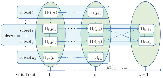
Figure 7.
Merging the detected special subsets i and j into a new subset .
3.3. Reconstruction of the Consistent Transformations
After obtaining the paired oblique projection matrix sequences in Section 3.2, the consistent transformation matrices can be reconstructed.
Firstly, the oblique projection matrix sequences in all subsets are classified into two groups based on whether they should be truncated or reserved. Usually, eigenvalues with low frequencies contribute more to system dynamics, and the related subsets are grouped into a new subset to be reserved, while the remaining subsets are to be truncated, as written in Equation (27).
where the second term in the above equation is derived from
Then, the consistent transformation at the grid point k can be reconstructed using the oblique projection matrix . Note that the matrix-valued function can be written as Equation (28) according to Equation (14).
New transformation matrix functions and can be reconstructed by a given matrix function .
The selected matrix function only needs to ensure that the matrix function has the same column rank as so that the vector space spanned by equals that by .
The reconstruction of the local transformation matrices and is realized by substituting the oblique projection matrix into Equation (29) point-by-point.
3.4. Algorithm Implementation
The implementation procedure of the proposed algorithm is summarized into 4 steps.
Algorithm input: the gridding-based LPV model pair with grid points.
Step 1: For k = 1 to , compute the local eigenvectors and formulate the oblique projection at each grid point.
Step 2: For k = 1 to , compute the distance metric . If most of the perturbed terms are out of the pre-specified tolerance , the step size between the k-th and -th points is too large. The grid points around there should be densely distributed, and the model order reduction process should be restarted from the beginning. If only a few of the perturbed terms are out of the prespecified tolerance , it indicates that two extremely close eigenvalue trajectories are detected, and there is no need to refine the grid points.
where
Step 3: For k =1 to , compute the metric distance and put the paired oblique projection matrix into the corresponding subset i.
where
Special cases described in Section 2.4 are detected that may belong to more than 2 subsets at the same time. The corresponding subsets should be merged into a new one. subsets will eventually be reduced to subsets. Each subset contains the oblique projection sequence and the coresponding eigenvalues.
Step 4: For k = 1 to , reconstruct the parameter-dependent transformations and .
Usually, subsets with low frequencies are selected to be retained. Merge the corresponding subsets that will be reserved into a larger subset assigned with the subscript . Then, the corresponding oblique projection is given as
Algorithm output: The reduced-order LPV model pair .
Remark 1.
The selection of is open, and the only restriction is given in Equation (30). A recommended choice is derived from a typical oblique projection matrix selected at grid point k.
where denotes the function of singular-value decomposition and is the rank of matrix .
Remark 2.
To maintain as much high-frequency information as possible, the modal residualization method can be used along with the proposed algorithm.
where
Note that transformation matrices and are derived by the oblique projection , which is complementary to in Equation (27).
Remark 3.
This oblique projection-based modal matching algorithm can also be applied to the balanced truncation technology, which is usually the last step necessary to obtain the final reduced-order model. Instead of eigenvalues and eigenvectors, this algorithm can help pair the Hankel singular values in the balanced truncation method.
4. Numerical Example
The proposed modal matching algorithm was tested by the typical LPV model order reduction method, modal decomposition, to demonstrate its effectiveness. The original LPV model was introduced in Section 2.1. The algorithm was run on a laptop with an AMD R7 5800H CPU and MATLAB 2020A. In this numerical example, it took about 8 s to run the algorithm and compute a reduced-order model from the original 48th order system.
The calculations were carried out according to the procedure given in Section 3. The algorithm was initiated with 48 subsets at grid point , where the corresponding oblique projections were calculated individually. The metric was then generated between the adjacent grid points. We randomly selected and for demonstration, and as shown in Figure 8, the paired oblique projections were easily identified by the Kronecker delta. The perturbation term between subsets 46 and 47 was noted to reach a certain threshold (the tolerance was set as ), and these two subsets were merged into a new subset.
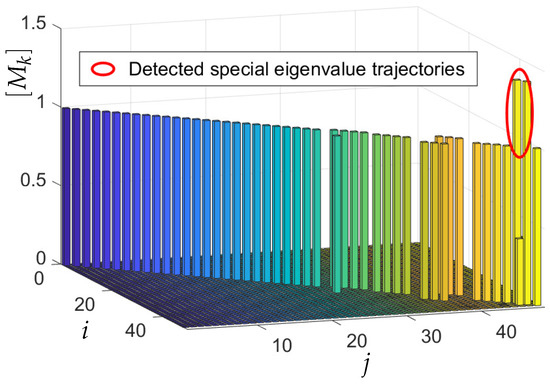
Figure 8.
The distance between grid points and , where multiple eigenvalues are detected in subsets 46 and 47.
After merging the special subsets with multiple eigenvalues and subsets with complex conjugate trajectories, the 48 subsets were reduced to 37 subsets. The paired trajectories are shown in Figure 9, where the detected special eigenvalue trajectories in red dots belong to subset 35. The corresponding real parts of the eigenvalue trajectories are shown in Figure 10. It can be observed that part of the trajectory is overlapped with the trajectories and as a form of complex–real transformations (the second special case given in Section 2.4) at different grid points. Such a situation is difficult to handle by smoothing the eigenvectors [4], while the proposed method skips this complex procedure and constructs consistent transformations, and , directly using the oblique projection .
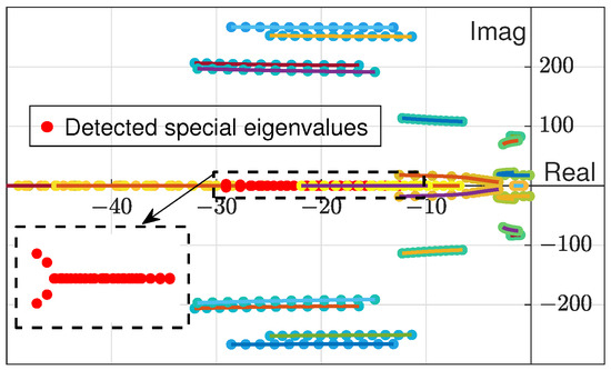
Figure 9.
Paired eigenvalue trajectories of the original model.
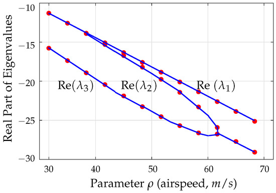
Figure 10.
Detected special eigenvalue trajectories in subset 35 (real part only).
Considering the frequency range that the flight dynamics and structural dynamics mainly contribute to, the system frequency of the reduced-order LPV model was limited to the range from 0.1 Hz to 50 Hz. Therefore, subset excluded 16 high-frequency trajectories, and 21 reserved subsets that consist of 32 state variables were selected to construct the oblique matrix function . The continuity of the reduced-order LPV system was verified by checking the parameter-dependent state matrix . Its interpolation performance is shown in Figure 11 by the randomly selected elements (6,10), (8,9), and (11,14) in the matrix sequences .
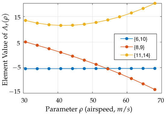
Figure 11.
Interpolation performance of the state matrix of the reduced-order model.
The -gap metric provides a measure of the similarity of the input-output mapping between two systems and , and they are identical if it is zero and completely different if one. A frequency-dependent formulation of this metric is given as the following equation [35].
The -gap metric between the original and the reduced-order models is given in Figure 12. There are additional models obtained by linear interpolation between any adjacent grid points. As shown in the figure, both the reduced-order model derived based on the oblique projection and the interpolation model between grid points have high fidelity. Note that only 16 high-frequency modes are truncated in the above process because the generated model would be further reduced by using the balanced truncation method to seek a complete model order reduction procedure for aeroservoelastic systems.
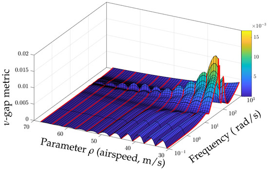
Figure 12.
-gap metric between the reduced-order model (32 states) and the original model.
To further verify the practicability of the proposed modal matching algorithm, the frequency range was limited between 0.1 Hz and 30 Hz, and then 16 subsets with 21 state variables were reserved. The modal residualization method is used to keep the information between 30 Hz and 50 Hz as much as possible. Figure 13 shows the output responses of the system for a doublet pulse input. The time-domain simulation shows that both the reduced-order models with 21 and 32 state variables have high-fidelity responses of the pitch rate q and the high-frequency acceleration relative to the original model. To better see the difference between the original system and reduced-order models, time-domain responses are also given in terms of errors. As shown in Figure 14, the model with 21 states has larger errors than the one with 32 states.
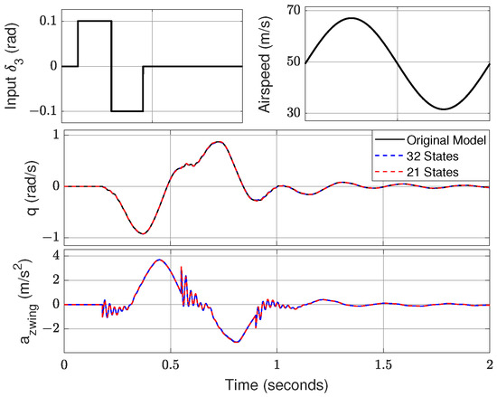
Figure 13.
Doublet pulse responses of the original system (48 states) and the reduced-order models (21 states and 32 states).
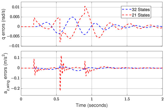
Figure 14.
Time response errors between the reduced-order models and the original model by doublet pulse input.
The frequency responses of two reduced-order models are also compared with the original system. Their Bode diagram plots on the grid point 5 at 44.2 m/s are shown in Figure 15. Note that it is inevitable to lose some information within 30 Hz and 50 Hz for the reduced-order model with 21 states, although this is not clearly shown in the time-domain simulations.
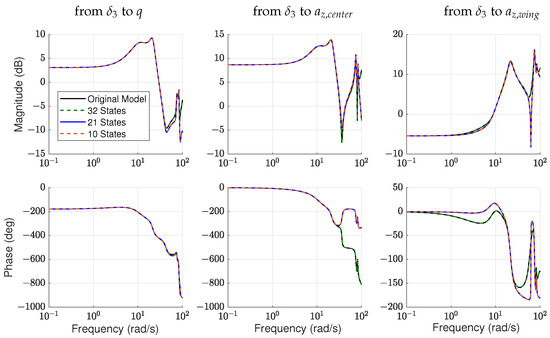
Figure 15.
Bode diagram of the original model and the reduced-order models from the input to outputs at the grid point 5.
Note that the proposed algorithm is described using the modal decomposition technology, which is the third step in the process of model order deduction. The idea of the oblique projection can also be applied to the balanced truncation technology. In this example, a reduced-order LPV model with 10 state variables is eventually obtained by further applying the balanced truncation method to the 21st-order LPV reduced-order model generated above. Its frequency responses are also given in Figure 15 and Figure 16, and the error caused by model order reduction is almost the same as the model with 21 states.
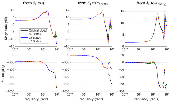
Figure 16.
Bode diagram of the original model and the reduced-order models from the input to outputs at the grid point 5.
5. Conclusions
A modal matching algorithm is proposed in this paper to help pair the eigenvalues and eigenvectors between the grid points in the process of LPV model order reduction. Different from the previous methods, the distance metric is based on the parameter-varying oblique projection. The newly defined metric contains , which makes the paired oblique projections easy to identify. At the same time, the perturbation term helps to detect the special trajectories and merge them into the same subset. The reduced-order LPV system is then obtained via the generated parameter-varying transformations and . The proposed algorithm can be applied to the LPV model order reduction of aeroservoelastic systems. The time response simulation shown in the numerical example indicates that the proposed modal matching algorithm can solve the state consistent problem well. It should be pointed out that the matrix-valued function is assumed to be diagonalizable, and systems that are expressed as the Jordan form cannot be handled well by this method. Another limitation is that the parameter variation is assumed to slow, and thus, the time derivative of the transform matrix is ignored in this paper. Model order reduction of LPV systems with fast varying scheduling parameters will be studied in our future work.
Author Contributions
Conceptualization, Q.L. and B.L.; methodology, Y.L. and W.G.; software, Y.L.; validation, W.G.; resources, Q.L. and B.L.; formal analysis, W.G.; writing—original draft preparation, Y.L.; writing—review and editing, all authors; supervision, B.L.; project administration, Q.L.; funding acquisition, B.L. All authors have read and agreed to the published version of the manuscript.
Funding
This work was supported by Shanghai Jiao Tong University under Grants AF4130042 and WF220841301.
Institutional Review Board Statement
Not applicable.
Informed Consent Statement
Not applicable.
Data Availability Statement
All data used during the study appear in the submitted article.
Acknowledgments
The authors would like to thank Julian Theis and Peter Seiler for providing the X-56A model.
Conflicts of Interest
The authors declare no conflict of interest.
References
- Ryan, J.J.; Bosworth, J.T. Current and Future Research in Active Control of Lightweight, Flexible Structures Using the X-56 Aircraft. In Proceedings of the 52nd Aerospace Sciences Meeting, National Harbor, MD, USA, 13–17 January 2014. [Google Scholar]
- Li, W.W.; Pak, C. Mass Balancing Optimization Study to Reduce Flutter Speeds of the X-56A Aircraft. J. Aircr. 2015, 52, 1359–1365. [Google Scholar] [CrossRef]
- Zhu, J.; Wang, Y.; Pant, K.; Suh, P.M.; Brenner, M.J. Genetic Algorithm-Based Model Order Reduction of Aeroservoelastic Systems with Consistent States. J. Aircr. 2017, 254, 1443–1453. [Google Scholar] [CrossRef] [PubMed]
- Theis, J.; Takarics, B.; Pfifer, H.; Balas, G.J.; Werner, H. Modal Matching for LPV Model Reduction of Aeroservoelastic Vehicles. In Proceedings of the AIAA SciTech, Kissimmee, FL, USA, 5–9 January 2015. [Google Scholar]
- Massey, S.J.; Stanford, B.; Jacobson, K.E. Progress on Flutter Analysis of the X-56A for the Third Aeroelastic Prediction Workshop. In Proceedings of the AIAA SCITECH 2022 Forum, San Diego, CA, USA, 3–7 January 2022. [Google Scholar]
- Grauer, J.A.; Boucher, M.J. Identification of Aeroelastic Models for the X-56A Longitudinal Dynamics Using Multisine Inputs and Output Error in the Frequency Domain. Aerospace 2019, 6, 24. [Google Scholar] [CrossRef]
- Ouellette, J.A. Aeroservoelastic Modeling of Body Freedom Flutter for Control System Design. In Proceedings of the AIAA Atmospheric Flight Mechanics Conference, Grapevine, TX, USA, 9–13 January 2017. [Google Scholar]
- Shi, P.; Liu, F.; Gu, Y.; Yang, Z. The Development of a Flight Test Platform to Study the Body Freedom Flutter of BWB Flying Wings. Aerospace 2021, 8, 390. [Google Scholar] [CrossRef]
- Perry, B., III; Cole, S.R.; Miller, G.D. Summary of an Active Flexible Wing program. J. Aircr. 1995, 32, 10–15. [Google Scholar] [CrossRef]
- Wang, Y.; Da Ronch, A.; Ghandchi Tehrani, M. Adaptive Feedforward Control for Gust-Induced Aeroelastic Vibrations. Aerospace 2018, 5, 86. [Google Scholar] [CrossRef]
- Schmidt, D.K.; Danowsky, B.P.; Kotikalpudi, A.; Theis, J.; Regan, C.D.; Seiler, P.J.; Kapania, R.K. Modeling, Design, and Flight Testing of Three Flutter Controllers for a Flying-Wing Drone. J. Aircr. 2020, 57, 615–634. [Google Scholar] [CrossRef]
- Takarics, B.; Patartics, B.; Luspay, T.; Vanek, B.; Roessler, C.; Bartasevicius, J.; Koeberle, S.J.; Hornung, M.; Teubl, D.; Pusch, M.; et al. Active Flutter Mitigation Testing on the FLEXOP Demonstrator Aircraft. In Proceedings of the AIAA Scitech 2020 Forum, Orlando, FL, USA, 6–10 January 2020. [Google Scholar]
- Pusch, M.; Ossmann, D.; Luspay, T. Structured Control Design for a Highly Flexible Flutter Demonstrator. Aerospace 2019, 6, 27. [Google Scholar] [CrossRef]
- Hjartarson, A.; Seiler, P.J.; Packard, A.; Balas, G.J. LPV Aeroservoelastic Control Using the LPVTools Toolbox. In Proceedings of the AIAA Atmospheric Flight Mechanics (AFM) Conference, Boston, MA, USA, 19–22 August 2013. [Google Scholar]
- Schmidt, D.K. Stability Augmentation and Active Flutter Suppression of a Flexible Flying-Wing Drone. J. Guid. Control Dyn. 2016, 39, 409–422. [Google Scholar] [CrossRef]
- Danowsky, B.P.; Thompson, P.; Lee, D.C.; Brenner, M.J. Modal Isolation and Damping for Adaptive Aeroservoelastic Suppression. In Proceedings of the AIAA Atmospheric Flight Mechanics (AFM) Conference, Boston, MA, USA, 19–22 August 2013. [Google Scholar]
- Tang, W.; Wang, Y.; Gu, J.; Sun, Z. LPV Modeling and Controller Design for Body Freedom Flutter Suppression Subject to Actuator Saturation. Chin. J. Aeronaut. 2020, 33, 2679–2693. [Google Scholar] [CrossRef]
- Theis, J.; Pfifer, H.; Seiler, P. Robust Modal Damping Control for Active Flutter Suppression. J. Guid. Control Dyn. 2020, 43, 1–13. [Google Scholar] [CrossRef]
- Zou, Q.; Huang, R.; Hu, H. Body-Freedom Flutter Suppression for a Flexible Flying-Wing Drone via Time-Delayed Control. J. Guid. Control Dyn. 2022, 45, 28–38. [Google Scholar] [CrossRef]
- Shamma, J.S.; Athans, M. Analysis of Gain Scheduled Control for Nonlinear Plants. IEEE Trans. Autom. Control 1990, 35, 898–907. [Google Scholar] [CrossRef]
- Wu, F.; Yang, X.H.; Packard, A.; Becker, G. Induced L2-Norm Control for LPV Systems With Bounded Parameter Variation Rates. Int. J. Robust Nonlinear Control 1996, 6, 983–998. [Google Scholar] [CrossRef]
- Moreno, C.P.; Seiler, P.J.; Balas, G.J. Model Reduction for Aeroservoelastic Systems. J. Aircr. 2014, 51, 280–290. [Google Scholar] [CrossRef]
- Moore, B.C. Principal Component Analysis in Linear Systems: Controllability, Observability, and Model Reduction. IEEE Trans. Autom. Control 1981, 26, 17–32. [Google Scholar] [CrossRef]
- Amsallem, D.; Farhat, C. An Online Method for Interpolating Linear Parametric Reduced-Order Models. SIAM J. Sci. Comput. 2011, 33, 2169–2198. [Google Scholar] [CrossRef]
- Benner, P.; Gugercin, S.; Willcox, K. A Survey of Projection-Based Model Reduction Methods for Parametric Dynamical Systems. SIAM Rev. 2015, 57, 483–531. [Google Scholar] [CrossRef]
- Yuan, W.; Zhang, X. Numerical Stabilization for Flutter Analysis Procedure. Aerospace 2023, 10, 302. [Google Scholar] [CrossRef]
- Shu, J.I.; Wang, Y.; Krolick, W.C.; Pant, K. Aeroelastic Reduced Order Model with State Consistence Enforcement. In Proceedings of the AIAA SciTech, San Diego, CA, USA, 3–7 January 2022. [Google Scholar]
- Theis, J.; Seiler, P.; Werner, H. LPV Model Order Reduction by Parameter-Varying Oblique Projection. IEEE Trans. Control Syst. Technol. 2018, 26, 773–784. [Google Scholar] [CrossRef]
- Luspay, T.; Péni, T.; Gőzse, I.; Szabó, Z.; Vanek, B. Model Reduction for LPV Systems Based on Approximate Modal Decomposition. Int. J. Numer. Methods Eng. 2018, 113, 891–909. [Google Scholar] [CrossRef]
- Villemagne, C.D.; Skelton, R.E. Model Reductions using a Projection Formulation. Int. J. Control 1987, 46, 2141–2169. [Google Scholar] [CrossRef]
- Burnett, E.L.; Beranek, J.A.; Holm-Hansen, B.T.; Atkinson, C.J.; Flick, P.M. Design and Flight Test of Active Flutter Suppression on the X-56A Multi-Utility Technology Test-Bed Aircraft. Aeronaut. J. 2016, 120, 893–909. [Google Scholar] [CrossRef]
- Wood, G.D. Control of Parameter-Dependent Mechanical Systems. Ph.D. Dissertation, Department of Engineering, University of Cambridge, Cambridge, UK, 1995. [Google Scholar]
- Lax, P.D. Linear Algebra. In Pure and Applied Mathematics; John Wiley & Sons: Hoboken, NJ, USA, 1996; pp. 112–114. [Google Scholar]
- Qian, J.; Chu, D.; Tan, R.C.E. Analyticity of Semisimple Eigenvalues and Corresponding Eigenvectors of Matrix-Valued Functions. Siam J. Matrix Anal. Appl. 2015, 36, 1542–1566. [Google Scholar] [CrossRef]
- Georgiou, T.T. On the Computation of the Gap Metric. In Proceedings of the 27th IEEE Conference on Decision and Control, Austin, TX, USA, 7–9 December 1988. [Google Scholar]


Disclaimer/Publisher’s Note: The statements, opinions and data contained in all publications are solely those of the individual author(s) and contributor(s) and not of MDPI and/or the editor(s). MDPI and/or the editor(s) disclaim responsibility for any injury to people or property resulting from any ideas, methods, instructions or products referred to in the content. |
© 2023 by the authors. Licensee MDPI, Basel, Switzerland. This article is an open access article distributed under the terms and conditions of the Creative Commons Attribution (CC BY) license (https://creativecommons.org/licenses/by/4.0/).