1. Introduction
Space surveillance is paramount in space situational awareness (SSA) due to its significant effect on military action and space operations. In this field, space targets refer to spacecraft in orbit, space debris, near-earth objects (NEO) and so on. Developments in space, electronics and processing technologies have made it possible to realize space target detection using different methods such as radar and optical systems. In 1990, the first software algorithm based on CCD images was designed to detect space targets [
1]. In the decades that followed, many experiments based on optical measurements demonstrated the feasibility and efficiency of this kind of method [
2,
3,
4]. However, in visual images, space targets are usually present in small sizes, and their intensity and shape are extremely variable due to the long imaging distance. As a result of the same imaging principles, the targets sometimes have a similar distribution to stars, especially when the exposure time is short. Thus, space target detection in a single image usually results in a lot of stars being falsely detected. In addition, stray lights, thermal noise, CCD imaging system noise and other interference may influence the detection. These factors converge to pose looming challenges for space target detection.
In recent decades, numerous studies have been dedicated to space target detection. Generally, a space target is presented as a light spot in an optical image, which is similar to the traditional infrared small target problem. Current small target detection methods can be broadly categorized into track-before-detect (TBD) methods [
5] and detect-before-track (DBT) methods [
6]. TBD methods usually utilize a sequence of frames and some prior knowledge of targets [
7]. Reed [
8] used a 3D matched (directional) filter to detect targets moving in uniform motion based on their shape and velocity. On this basis, the 3D double directional filter [
9] and improved 3D directional filter [
10] were then proposed to improve the detection ability for weak targets. Moreover, a modified partial differential equation [
11] and support vector machines [
12] have been used to suppress the background and remove false alarms. Compared with TBD methods, DBT methods require fewer assumptions and prior knowledge, so they are among the most commonly applied methods in engineering. For detection in single images, image binarization is a widely applied method. Stoveken [
13] summarized several methods to identify objects. Methods including star catalogs, object characteristics and median images are used to realize image binarization. On this basis, Virani [
14] detected and tracked objects using a signal-to-noise ratio (SNR) threshold and a Gaussian mixture-based probability hypothesis density (GM-PHD).
One of the earliest programs dedicated to detection was the Lincoln Near Earth Asteroid Research (LINEAR) program. A binary hypothesis test (BHT) was utilized to generate a binary map, where the value of detected targets is 1 [
15]. Zingarelli [
16] proposed a new method combining local noise statistics and a multi-hypothesis test (MHT) to reject outliers. Hardy [
17] found that an unequal cost MHT achieves better performance than an equal cost MHT when the potential intensity of targets occupies a large range. Tompkins [
18] used MHTs and parallax to find the difference between the point spread functions (PSFs) observed from a star and Resident Space Objects (RSOs).
Another more computationally complex method is a matched filter. The main aspect of a matched filter approach is the match between the observed data and the expected PSF. Among these methods, the SExtractor software is widely used for object detection within the SSA community [
19]. Bertin [
20] has conducted further work to apply and update the software over the years. Murphy [
21] used the multi-Bernoulli filter to detect space objects with a low SNR. Furthermore, they utilized prior knowledge to design a bank of matched filters, and the filtering results were transformed as the measurement likelihood for a Bayesian update and subsequent detection [
22]. Lin [
23] researched the essential features of targets and proposed the multiscale local target characteristic (MLTC) to judge whether a local area contains a target.
In other small target detection fields, the max-mean, max-median [
24], top-hat [
25], two-dimensional least mean square (TDLMS) [
26] and other methods are widely used to suppress backgrounds and enhance targets. Recently, methods based on the human visual system (HVS) such as the local contrast measure (LCM) [
27], improved local contrast measure (ILCM) [
28], relative local contrast measure (RLCM) [
29], neighborhood saliency map (NSM) [
30] and weighted strengthened local contrast measure (WSLCM) [
31] have been introduced for target detection. Some methods regard the detection task as a two-class recognition problem. Qin [
32] addressed the problem with a novel small target detection method based on the facet kernel and random walker (FKRW) algorithm.
In latest developments, many methods based on deep learning have been networks (RCNNs) [
33,
34] and Yolo [
35,
36,
37,
38], SSD [
39] and DEtection TRansformer (DETR) [
40]. These methods can learn features from huge amounts of data rather than handcrafted features so that they perform well when the data are rich and unique. However, the size of the space target is small and their texture information is little. Therefore, popular methods using deep learning are not suitable for the detection of space targets. Jia [
41] proposed a method based on the concept of the Faster R-CNN to detect and classify astronomical targets with certain image sizes. Xi [
42] proposed a space debris detection method using feature learning of candidate regions (FLCR) in optical image sequences. The method still suffers difficulties in using the spatial features of dim and small objects sufficiently. In addition, some methods based on deep learning have been used for small targets by generating backgrounds and separating small targets, including semantic constraint [
43], denoising autoencoder [
44], generative adversarial network (GAN) [
45,
46], a spatial-temporal feature-based method [
47] and a feature extraction framework combining handcrafted feature methods and convolutional neural networks [
48]. Li [
49] designed a network named BSC-Net (Background Suppression Convolutional Network) to realize the background suppression of stray lights in star images. However, this method is still unable to filter out weak targets.
The above methods still suffer difficulties which need to be overcome when used in space target detection.
- 1.
Even though the intensities of the same target in different images or different targets in the same image change dramatically, they share high similarities with the distribution. However, it is difficult for traditional methods based on theoretical models to summarize a generalized distribution function of space targets that covers different situations.
- 2.
In the stage of the final target confirmation, the thresholds are usually set based on the information from the global image. This can barely balance the detection of weak targets and a decrease in false alarms.
- 3.
A star image contains a large number of targets that can be used to build a dataset, which provides a good foundation to build a deep convolutional neural network that can approximate the distribution function of different targets. Due to the diverse detectability of optical systems, even the images pointing to the same sky area contain different magnitudes and quantities of stars. Thus, although there are thousands of targets existing in an image, not all of them are certain, which results in a higher cost of annotation for a full image and lower validity of detection.
- 4.
The common end-to-end detectors based on CNN [
50] do not perform well for small target detection. Besides, most of the structures of existing networks are complex and bring high requirements for in-orbit hardware resources.
To address these problems, this paper aims to develop a novel and low-cost method for space target detection based on distribution characteristics, which can potentially be used in actual in-orbit service. In this paper, a CNN is applied to learn the distribution of targets automatically with no need for a certain matching function or criteria. Proposals are separated from the background, located by finding an intensity higher than the local area, and confirmed depending on whether they follow a particular distribution. Real data are used to test the proposed method. The experimental results demonstrate that our method is simple and effective for targets with diverse signal-to-clutter values. Furthermore, the proposed method shows a significant superiority over baseline methods.
As a whole, the contributions of this paper can be summarized as follows:
- 1.
A method is presented to detect space targets by modeling the global detection of an image as local two-class recognition of several candidate regions so that manual labeling for a full image is not required.
- 2.
We design a small architecture of the CNN to realize automatic feature extraction and target confirmation, which avoids the problem of threshold setting for the final target confirmation. Furthermore, the architecture can potentially be used in actual in-orbit services because it is easy to implement and requires only a low cost in terms of computing resources.
- 3.
We added a module of information guidance to improve the detection ability. The former is applied to each candidate region to reduce the difference in intensity among targets, which confers a better generalization ability to the network. Furthermore, the latter is added to provide extra features. In this way, the interference caused by pixels in the non-central area is further reduced and the distribution characteristics of the target are enhanced. This method shows good performance in experiments.
The remainder of this paper is organized as follows. In
Section 2, we explain the target detection method based on a CNN. In
Section 3, we introduce the implementation in detail. Extensive experimental results and discussions are given in
Section 4, and the conclusions are provided in
Section 5.
2. Proposed Method
2.1. Problem Description
Traditional methods usually design features and standards to distinguish targets from backgrounds. However, an image contains not only a large number of star targets and space targets whose intensity and size are extremely variable, but also contamination and noise such as smear effects and stray light [
23]. Methods based on the normal threshold policy, such as thresholding, pyramids and morphology operations, can hardly maintain robustness when facing different complex backgrounds. A large threshold means a loss in the detection ability for weak targets. A small threshold may result in many false alarms and target region connections.
Generally, when the relative motion between the optical system and the target is small during the exposure time, the intensity of a star image
f can be regarded as a combination of the target
t and noise
n:
where the noise
n includes background and space environmental effects,
is the center coordinate of the target,
S is the scale coefficient and
is the standard deviation of the PSF.
However, targets, including space targets and star targets, usually do not follow the standard distribution in practical engineering, because when there is stray light in the image, some targets in the affected area may have a low signal-to-noise ratio and their original distribution characteristics will be overwhelmed by noise. At the same time, the camera and space target in the space-based observation system may move, which not only results in a certain image displacement of the target during the exposure time but also imposes a negative impact on the target distribution. It is difficult to summarize a generalized distribution function of space targets and to set thresholds that cover different situations. Even though the stars and targets are diverse in shape and intensity, the targets maintain the following characteristics:
- 1.
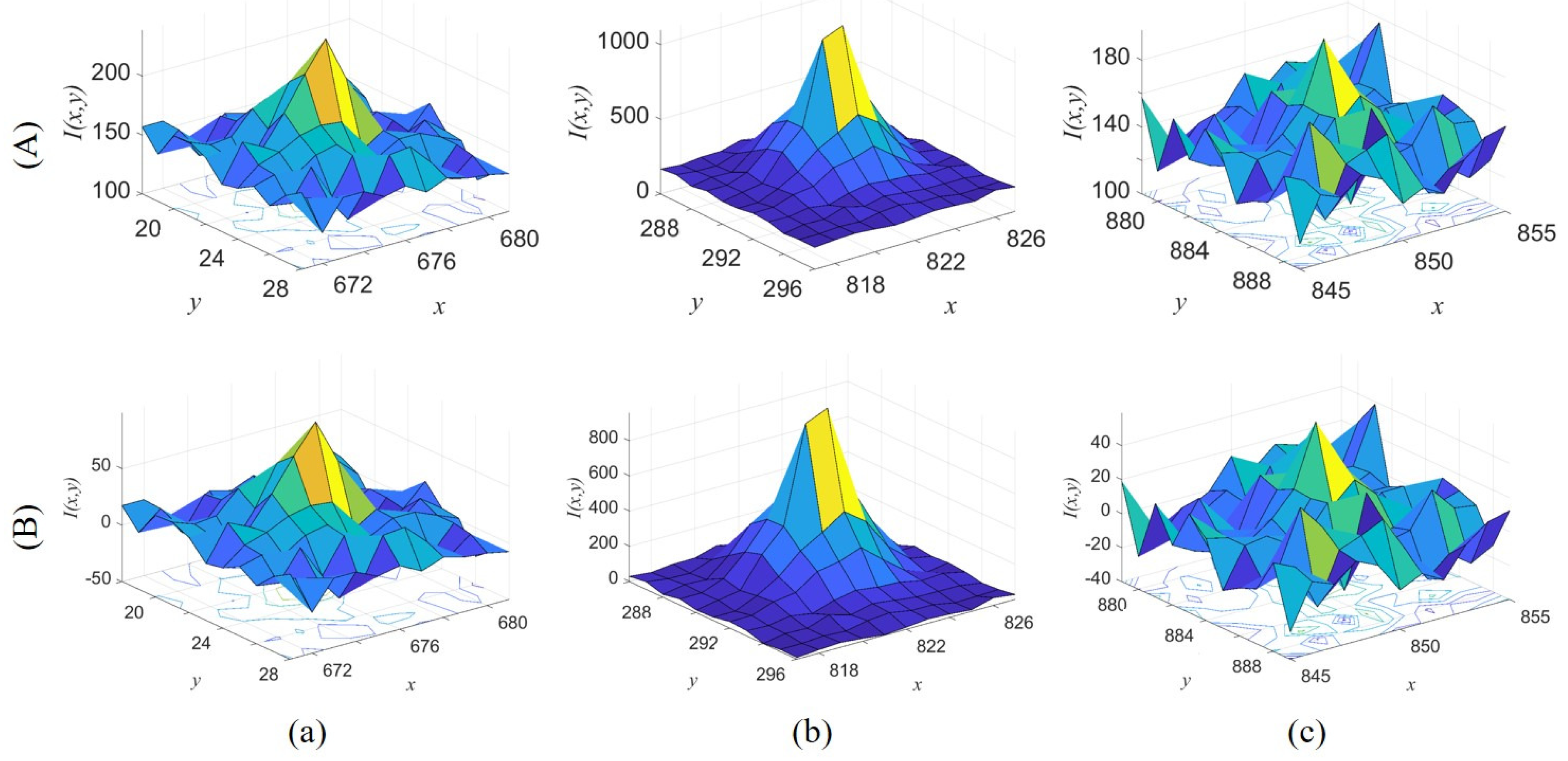
The target center is the local maximum.
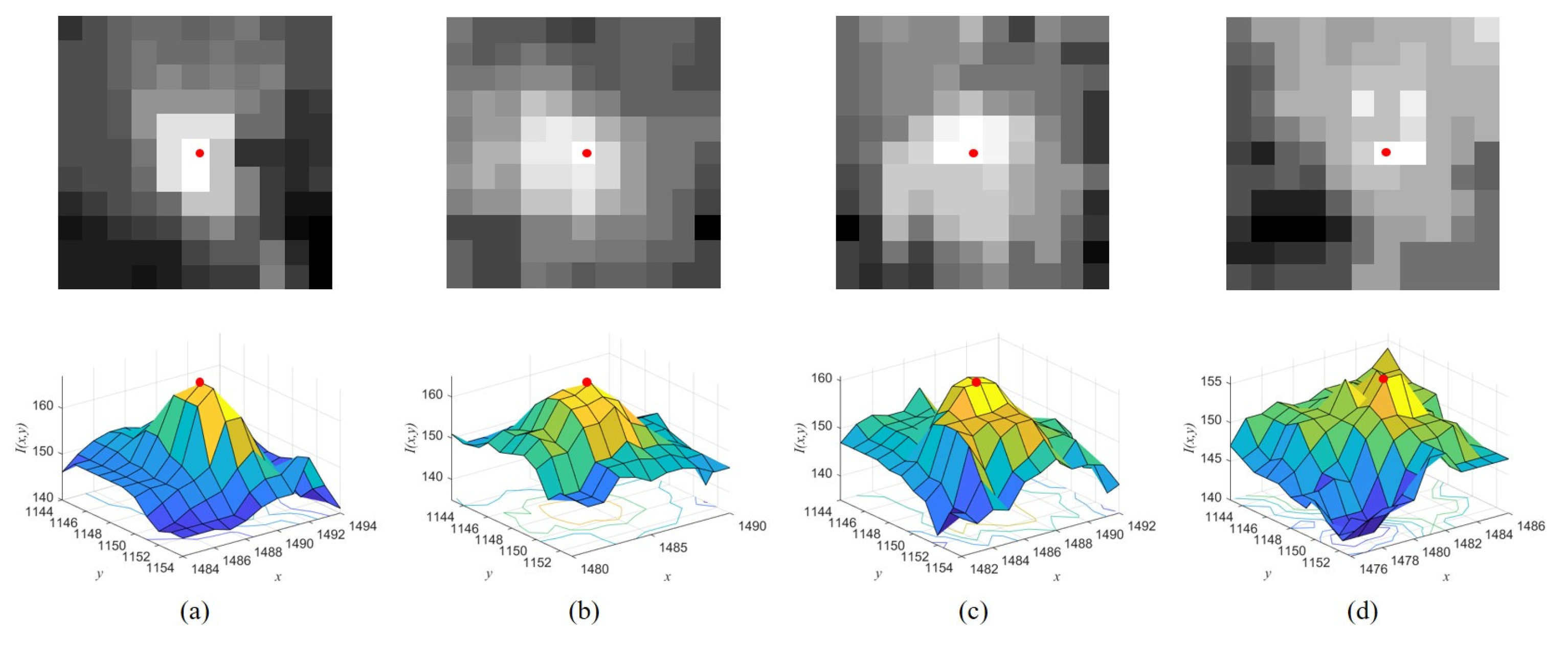
Figure 1 shows the original images and corresponding intensity distribution of the same target with low SCR values in different frames, where the center of the target in each image is marked in red. The distribution of the target is easily influenced by the noise (
Figure 1c) and the PSFs of close stars and other targets (
Figure 1d). The intensity value of each pixel inside the target region is the superposition result of the target and other interference; thus, the target center still retains its saliency unless it is submerged.
- 2.
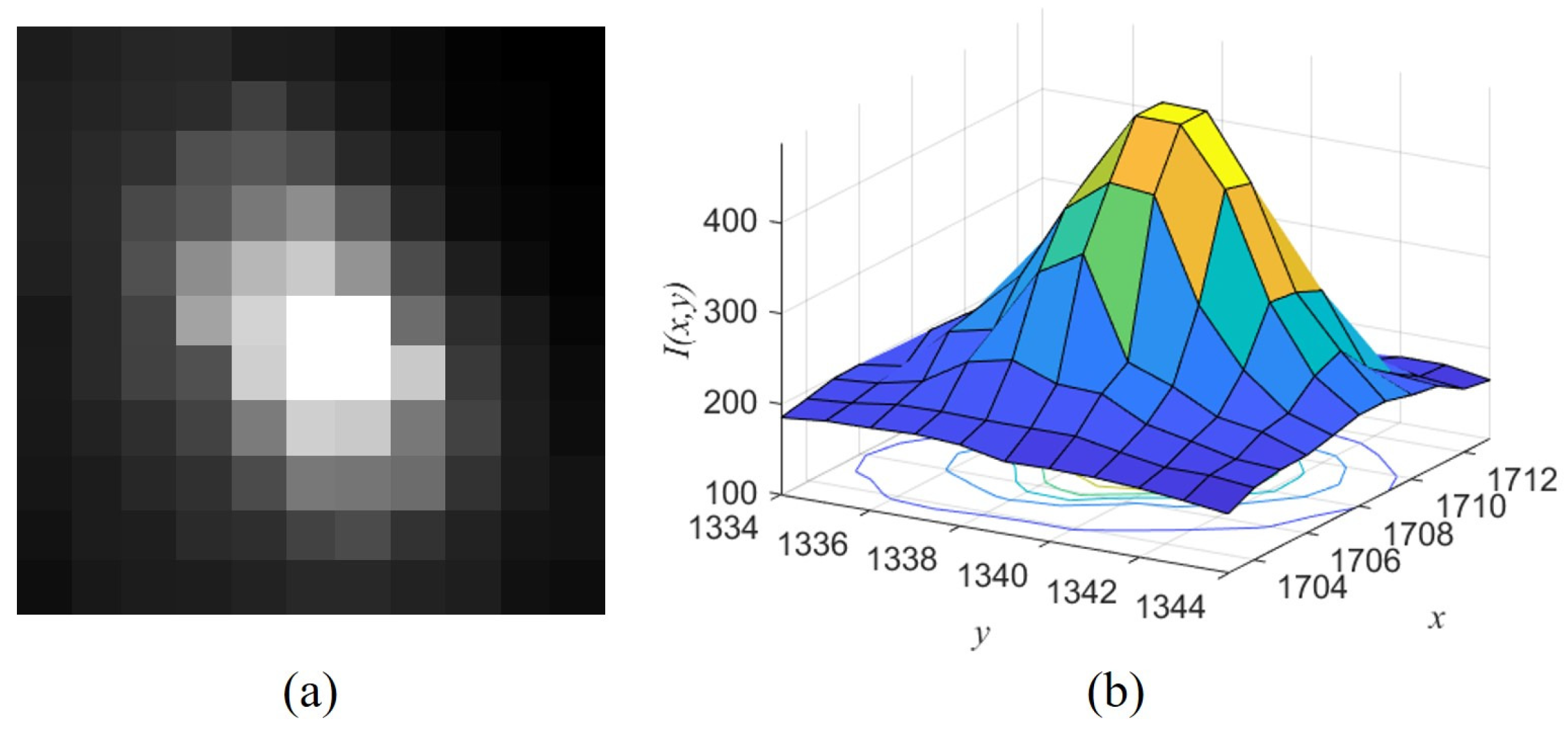
When the target has no fast relative motion, its distribution approximates a Gaussian distribution. The difference is that the actual distribution extends in the direction of its motion because of motion blur if the exposure time is long or the target has a high speed, as shown in
Figure 2.
Considering that there is no relative public dataset, another problem that needs to be solved is the construction of the dataset. There are differences among optical systems that affect image quality, representation of stars and targets and identification of stars and targets. Even images of the same patch of sky contain different amounts of stars and targets because of different cameras or parameters. It is difficult to realize labeling of the whole image. In addition, even a simulation can hardly describe all of the distribution because of the diversity of targets regarding shapes, sizes and intensities.
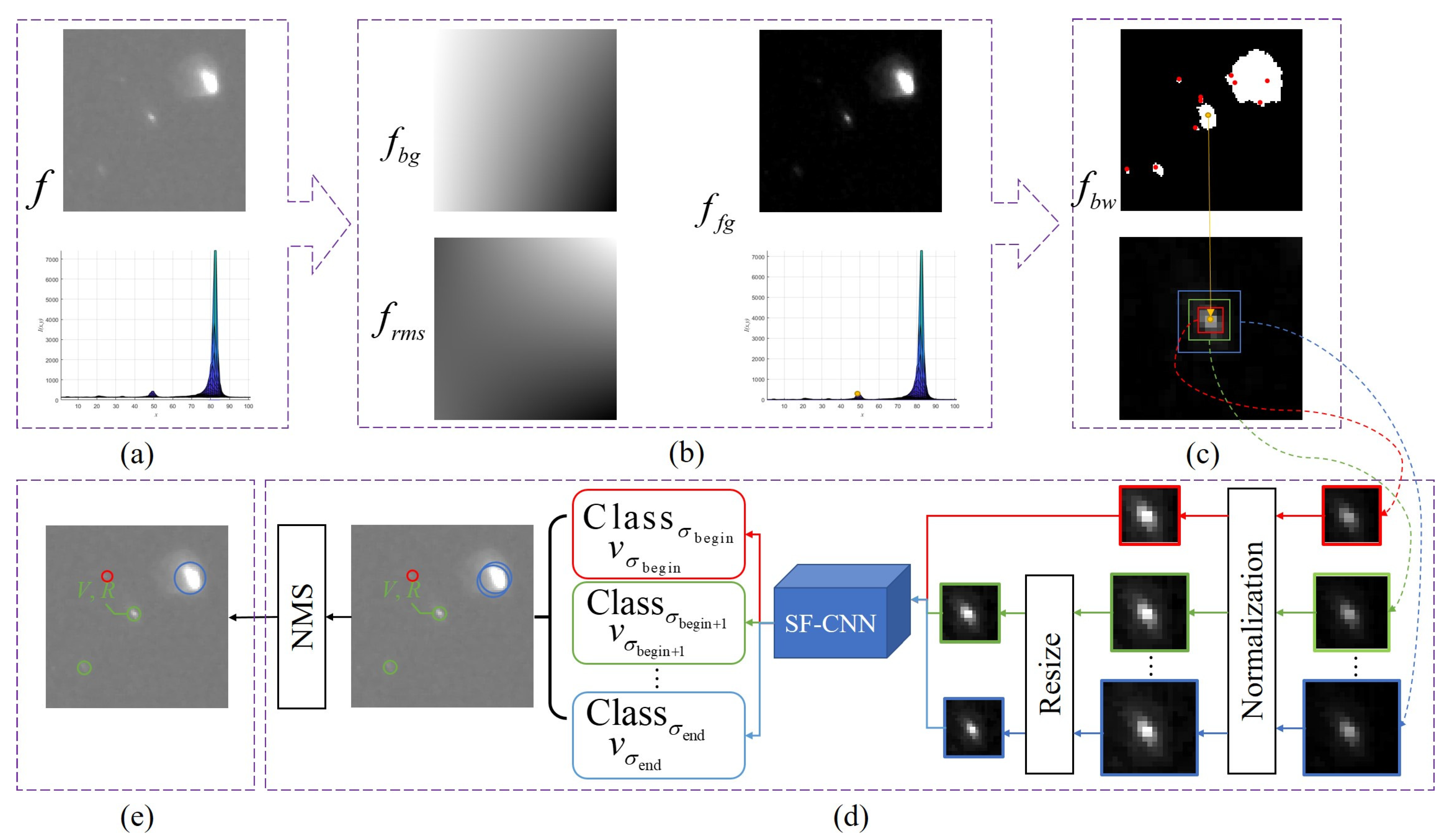
Thus, we proposed a method composed of the following three main phases as depicted in
Figure 3. All displayed images have been stretched with contrast. The first phase is a preprocessing stage, where a set of techniques are applied to the image, resulting in a background-removed image. The second phase is the region proposal search, where local maximum points in the foreground are extracted and regions with different sizes (marked in red, green and blue) around these points are formed as proposals. The third phase is the certification of proposals with a specially designed CNN. The detected targets are shown in different colors according to the size with the highest confidence.
2.2. Preprocessing Stage
The method used in SExtractor [
19] is introduced to suppress the background due to its effectiveness and suitability for this research. Grids are set to divide a star image into background meshes. For each mesh, its local background histogram is clipped iteratively until convergence at
around its median. During the process, if
drops by less than 20%, the mean of the clipped histogram is regarded as the background value. Otherwise, the local background
is estimated with:
The background map and the root mean square (rms) map are then generated by a bilinear interpolation between the meshes of the grid. The mesh size is set as 32 here. The foreground
, mainly including stars and targets, is segmented from the background
as follows:
The RMS map is applied to binarization as follows:
where
is the binarization image and
is the RMS map.
2.3. Region Proposal Search
According to the previous analysis, there is high relevance between target centers and local maximum points in an image. This feature can be applied to find region proposals of targets. Local maximum values in an image are extracted by an expansion operation:
where
is the expanded image and
is the region of the expansion operation, which is decided according to the minimum search distance between targets.
It is difficult to distinguish a target with a radius of 1 from thermal noise; thus, the smallest pixel-level radius for which people can judge whether or not a region contains a target is 2. Thus, we set
to 5 (
), i.e., the searching radius is 2, to maintain the sensitivity of the method for two close targets in this paper. The point set of suspected center points
is defined as
Regions with different sizes around each point will be extracted as proposals. A smaller may result in more proposals containing only the background; thus, these proposals will be classified by the CNN designed in the next subsection.
2.4. Target Detection with an SF-CNN
For each searched region proposal, we need to confirm whether there is a target present. In this way, target detection in the whole image is transferred into the recognition of a sub-image. In order to solve the problem of simple segmentation thresholds when using traditional methods and to improve the generalization ability for targets of different shapes, a method based on deep learning is considered. With the limitations of hardware resources and calculating pressures in orbit, we attempt to use a simple and small CNN called SF-CNN rather than state-of-the-art deep learning methods. This network is trained to obtain a small model C that classifies a sub-image into a target or non-target.
After the preprocessing stage and region proposal search, the input of the model C is each processed proposal, , and the output is the predicted class, i.e., target (=1) or non-target (=0) as well as a corresponding confidence value (the output of C). Parameter training will be stopped until the loss stops decreasing and approximately converges at a constant value. In that way, the trained C is considered to have learned the distribution of small targets in the dataset so that it can be directly used to predict the class of inputs unless the distribution of targets is severely impacted by the background or nearby stars in the image.
There is no prior information on targets or stars; thus, for each suspected center point
, proposals of different sizes are extracted to obtain the size information of the target. The value map
V and radius map
R are generated as:
where
is the confidence value of point
in size
. If the center of a proposal is not the maximum,
equals 0.
is set according to the information of the optical system, and 11 is chosen in this paper.
There can be more than one suspected point in the region of a target; thus, to remove redundant targets in the same proposal, we apply a non-maximum suppression (NMS) operation:
where
is the maximum of
V within radius
R. A point whose
V value is 1 will be regarded as the center of a target. The implementation details are provided as follows.
4. Experimental Results
The model described above was applied to detect targets in star images. The CNN was implemented in Python 3.7 on a PC with a 16 GB memory and a 1.9 GHz Intel i7 dual CPU. During the experiments, we used PyTorch to compute the convolution with a learning rate of 0.001. In the training process, stochastic gradient descent (SGD) was used for optimization. The learning rate was 0.001, the momentum was 0.9 and the batch size was 10.
4.1. Experimental Settings
(1) Evaluation metrics
(a) Classification metrics
In this paper, the
score is selected to reflect the classification ability of the network. It is an indicator used in statistics to measure the accuracy of binary classification models. Precision refers to the proportion of the number of correctly classified positive samples with respect to the total number of classified positive samples. Recall rate refers to the proportion of the number of correctly classified positive samples among the positive samples. They are calculated as follows:
where
(true positive) represents the number of correctly classified positive classes in positive samples,
(false positive) represents the number of incorrectly classified negative classes in positive samples and
(false negative) represents the number of incorrectly classified positive classes in negative samples. The accuracy rate reflects the accuracy of the overall classification of the network.
takes into account both the precision and recall of the classification model. It can be seen as a harmonic average of model accuracy and recall, with a maximum value of 1 and a minimum value of 0. The calculation is as follows:
(b) Detection metrics
SCR is a common metric used to reflect the saliency of targets. The SCR of the
ith target is defined with the information of the target and the surrounding area. The calculation is as follows:
where
is the mean intensity of the target and
and
are the mean value and standard deviation of the intensity of the area, respectively.
The true positive rate (TPR) and false positive rate (FPR) are defined as
where TD is the number of true targets detected, ND is the number of targets detected, FD is the number of false targets detected and NT is the total number of pixels in the area.
(2) Dataset
(a) Training data and validation data
There is no public dataset related to the research in this paper; thus, star images taken by two space-based telescopes or five ground-based telescopes under different imaging conditions were used to construct the dataset. For a determined target, the region of
around the target is extracted and normalized to the data. The dataset consists of 3408 sub-images which were randomly selected from more than 800 star images. The dataset was divided into a training set and a validation set according to the ratio of 7:3. There are many possibilities for the distribution of non-target areas; thus, in order to avoid paying too much attention to negative samples during training and convergence speed-up, the training set contains 1428 positive samples and 956 negative samples and the validation set contains 578 positive samples and 446 negative samples, as shown in
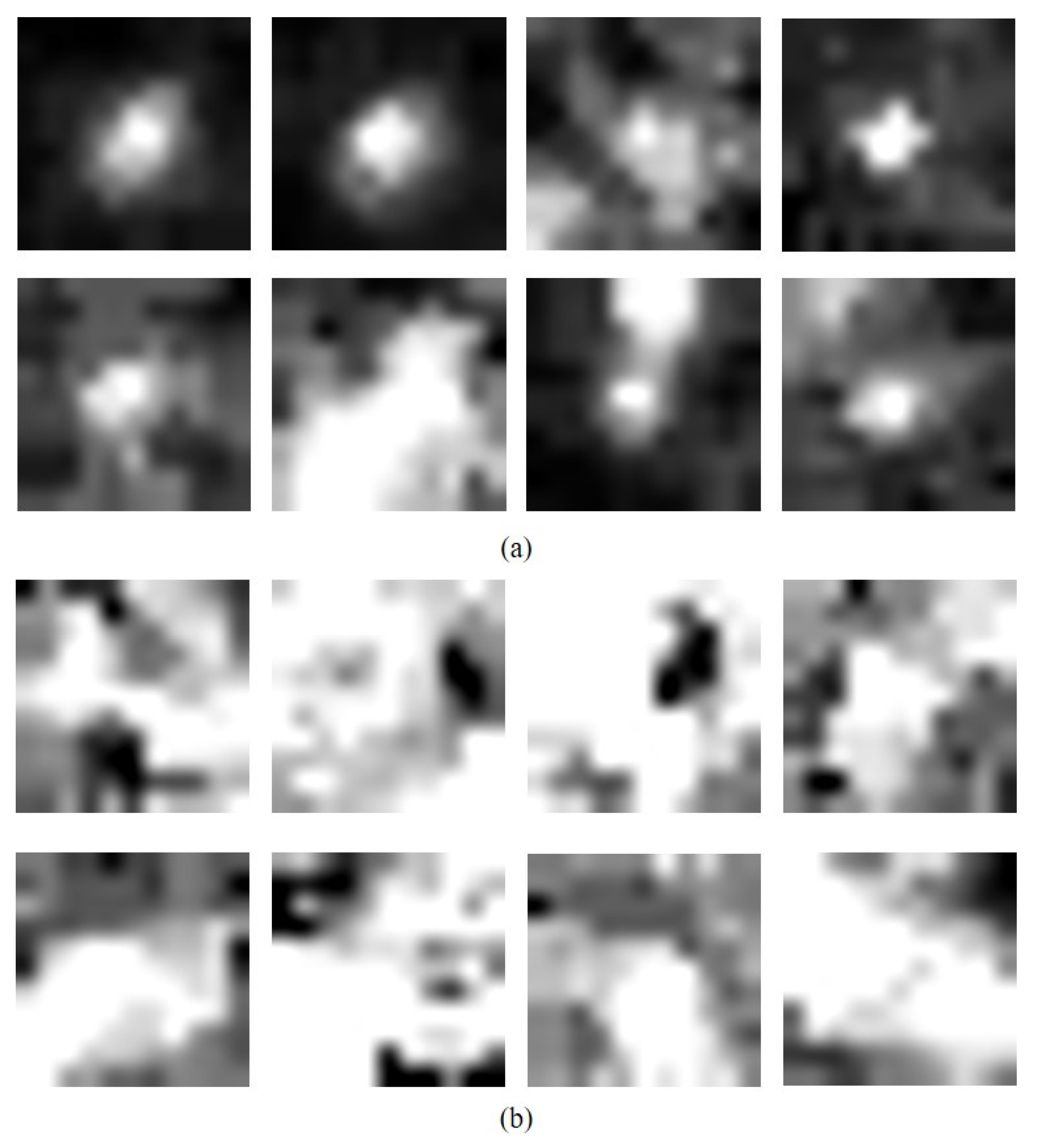
Figure 5. Among these, the positive sample includes the following three cases: (1) targets moving in different directions, i.e., targets extend and distribute in different directions; (2) targets with different sizes and significance and (3) images containing other stars or targets. In this way, overfitting can be reduced as much as possible.
(b) Test data
We used four new groups of star image sequences acquired by another ground-based space surveillance telescope to verify the performance of the proposed method.
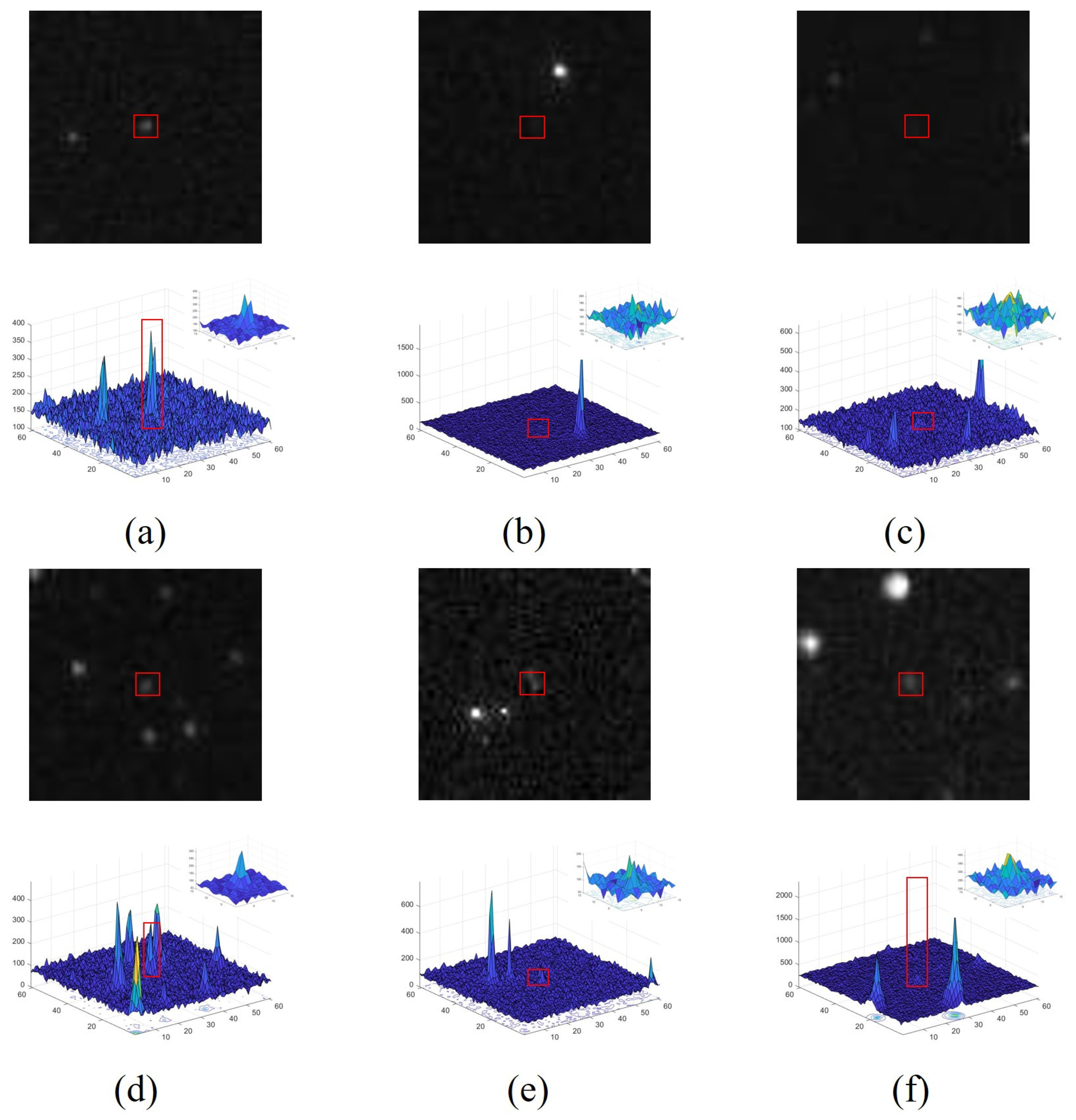
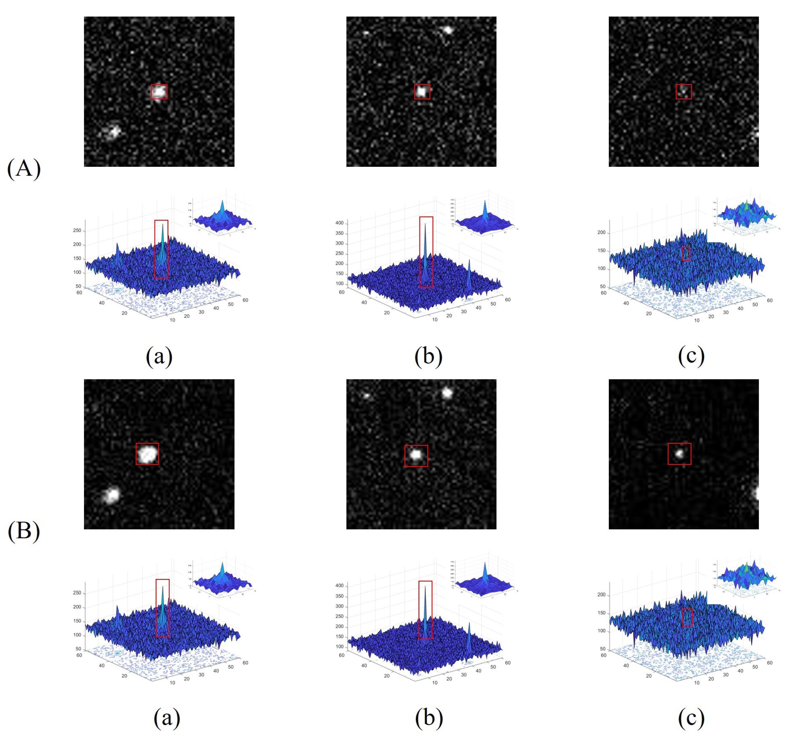
Table 2 shows the key parameters of the telescope during data acquisition. Nine typical targets with various SCR values in the sequences are summarized in
Figure 6 and
Figure 7. To process the algorithm quickly when determining target information and interference, small image subsets of 201 × 201 pixels around the targets are extracted from each frame and used to form new sequences, denoted as sequence 1 to sequence 9. Details of the targets and backgrounds are listed in
Table 3, where information is calculated according to the true targets and their nearby areas whose sizes are slightly larger than the target radius in each frame.
(3) Baselines
To validate the detection ability of our method, it was compared to several state-of-the-art traditional small target detection methods. Although some mainstream deep learning techniques outperform conventional non-deep learning methods, these methods cannot be directly applied to this problem for the following reasons: (1) it is difficult to obtain correct labels in the whole image with prior information; (2) most of the deep learning methods contain several max-pooling layers, which are not applicable to small targets; (3) if the deep learning methods are only used for two-class recognition, their complicated structure may require more time for training and lead to inferior detection capability and (4) the deep learning methods need more computing resources, which places more pressure on the in-orbit system. Considering the cost of manual labeling for a full image and realizability in actual engineering, common deep-learning-based methods were not chosen in this paper. Methods based on global binarization (max-mean, RLCM, NSM and WSLCM), a method based on local binarization (FKRW) and local theoretical model-driven methods (SExtractor and MLTC) were utilized as baseline methods.
4.2. Comparative Analysis of the Processing Stage
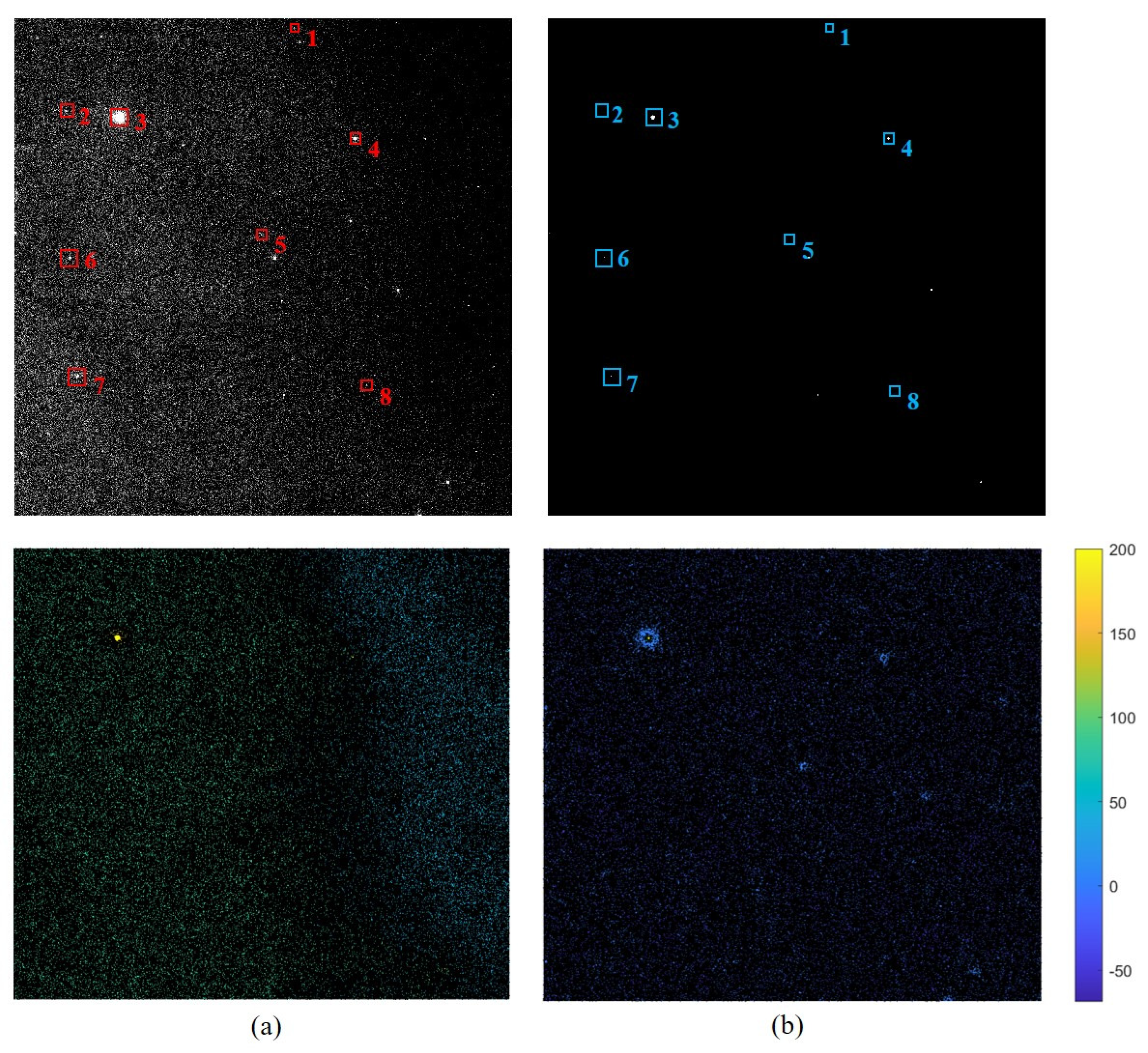
To verify the influence of the preprocessing stage on the star image and targets inside, an image disturbed by strong stray light was selected for preprocessing. The image size is
, and the comparison before and after the processing stage is shown in
Figure 8. Since the depth of the original image is 16 bits, to compare the effects of processing more reasonably, the images before and after processing are stretched to the same gray range of
. In the contour map, to better reflect the gray change of the background, parts of the image with a gray value higher than 200 are truncated. There is a large area of uneven interference in the original image. The interference in the processed image is obviously removed and the background is close to 0. Furthermore, eight stars with different significances in different positions and different degrees of interference were selected for comparison.
Figure 9 shows the images and corresponding gray distribution of three stars (Star 1, Star 4 and Star 8) before and after processing. The processed image better reflects the distribution of the target versus the background, i.e., the original distribution of the target. However, because the algorithm mainly roughly estimates the background, it is difficult to filter the interference of inclusions in the target. The processing effect is quantitatively analyzed in
Table 4, including the number of candidate points in the figure and the SCR value of the target. It can be seen that preprocessing has less influence on the image details and less interference with the original distribution of the target and its region. On the other hand, because a large area of interference is filtered out, the false extraction of candidate points in the bright–dark junction area is greatly reduced, which increases the processing speed of the algorithm.
4.3. Comparative Analysis of Ablation Experiments
Furthermore, ablation experiments were conducted and the results are shown in
Table 5.
Compared with no normalization, traditional cross entropy loss and the no guidance mode, the network combining normalization, bias loss and the addition of guidance information achieves the highest score, which means that the network can effectively balance the classification precision and recall rate.
4.4. Comparative Analysis of Experiments for Different Targets
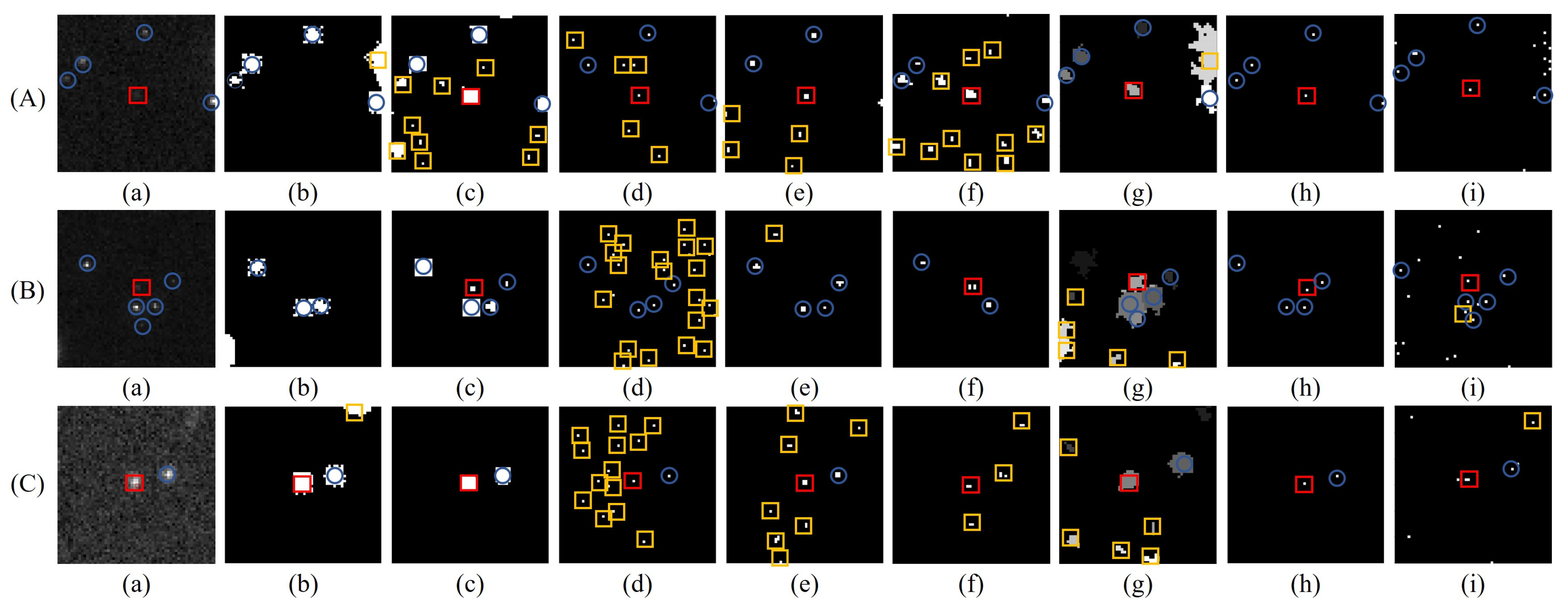
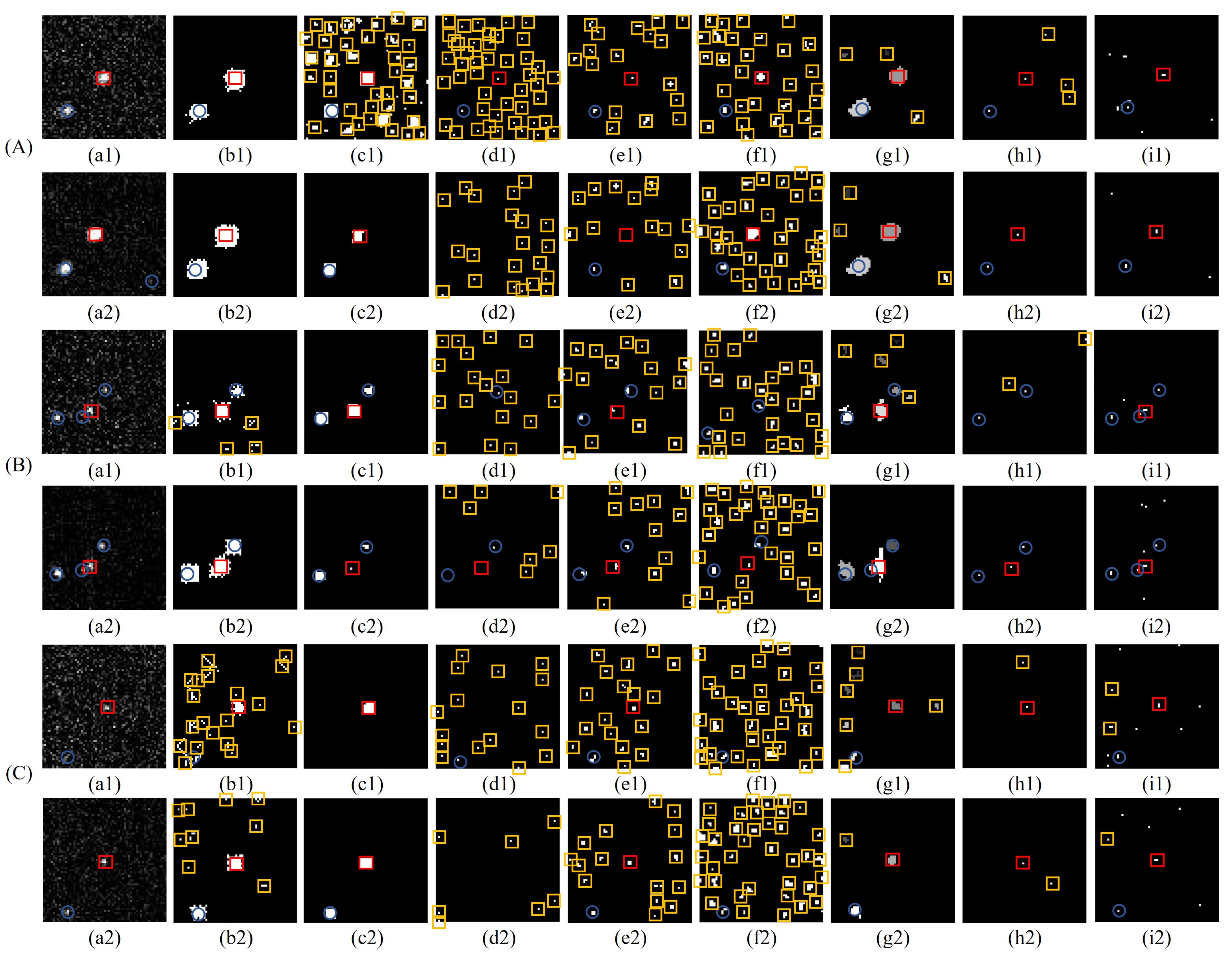
In order to demonstrate the generalization of the proposed method, sequences containing different targets with various backgrounds, shapes, sizes and intensities are processed using the above methods. Three typical targets in different sequences with a large range of SCRs (target 3, target 4 and target 6) ertr randomly selected from the dataset, and
Figure 10 shows a comparison of the corresponding saliency maps and detection results with different methods. Here, the space targets and star targets detected correctly are labeled individually in red boxes and blue circles, and the yellow box represents a false alarm. The saliency maps of max-mean, RLCM, NSM, WSLCM and FKRW are the results of threshold segmentation. The MLTC column presents the final detection results, and the column of the proposed method only shows the proposals. For each method, the same parameters were used during the detection of a sequence.
Intuitively, false alarms and misdetection frequently occur in RLCM, NSM, WSLCM and FKRW due to the relatively unstable performance of background suppression. Max-mean adopts target enhancement and performs better with respect to false alarms. However, this method may further reduce the saliency of targets present in a low-contrast environment, as shown in
Figure 10(B(b)). Instead, SExtractor and MLTC focus on the distribution of targets rather than local saliency, so fewer false alarms and misdetection occur.
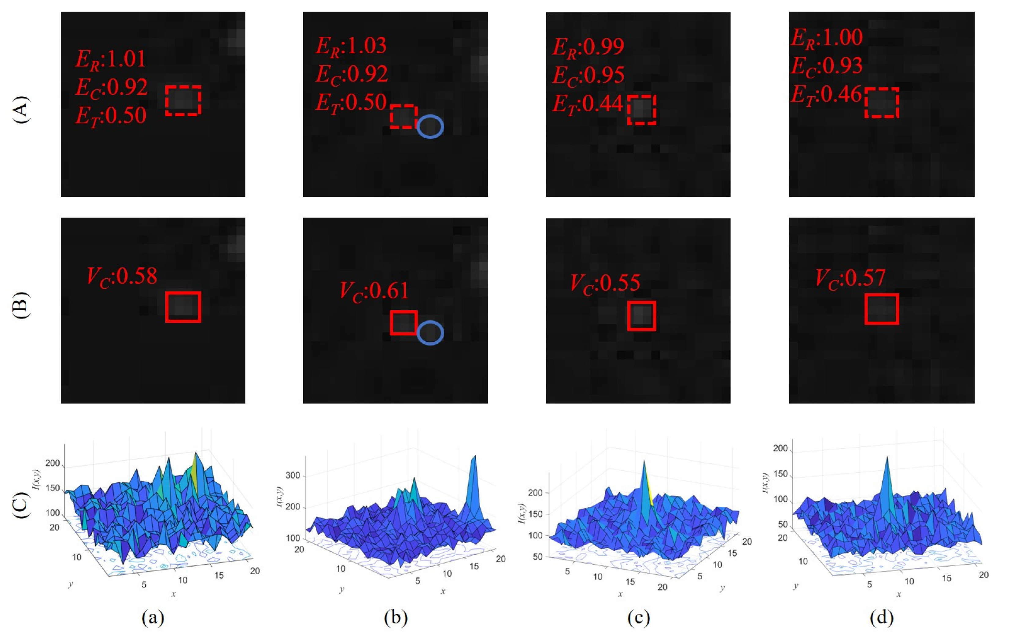
Figure 11 shows four typical undetected targets of MLTC and the calculation results of MLTC and the SF-CNN are given. When targets deviate from the ideal distribution due to them moving (
Figure 11a), interference from the background (
Figure 11b) or their small size (
Figure 11c,d), the above two methods are also subject to the problem of threshold setting. The proposed SF-CNN follows a similar principle of target estimation with intensity distribution. The main difference is that the SF-CNN is data-driven rather than model-driven. Thus, the SF-CNN is more appropriate for targets with different shapes and less likely to be influenced by the background.
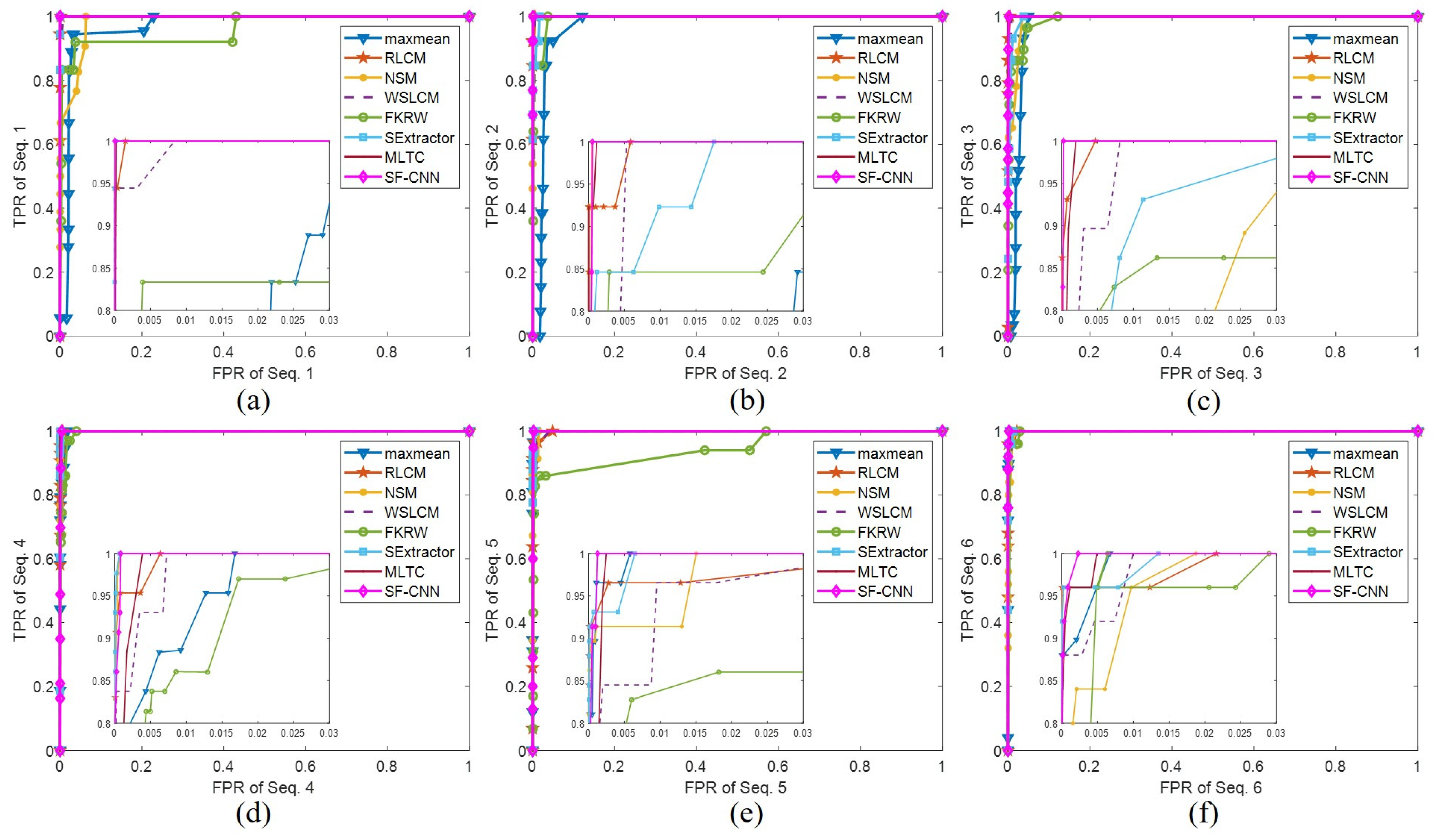
The receiver operator characteristic (ROC) curve for sequence 1 to sequence 6 is shown in
Figure 12 to further reveal the advantages of the proposed method over the other seven methods. From the figure, we can see that the proposed algorithm achieves the lowest FPR for the same TPR in most cases.
The statistical results of the target detection methods are listed in
Table 6. It should be noted that the same parameters are shared in different sequences when the MLTC and the SF-CNN are applied. In contrast, the parameters of the baseline methods in each sequence are confirmed after balancing the TPR and FPR. For each sequence, different values of each parameter are set to some images, and the values corresponding to the maximum acceptable FPR are selected after visual inspection. Furthermore, the TPR is determined at these parameter values. On the whole, the highest TD and TPR for all sequences achieved by our method indicate that it can stably detect targets with different SCRs and perform better than baseline methods.
Finally,
Table 7 lists the average time required for detection in a single image. Compared to the baseline methods, the proposed method shows great advantages in processing time. Furthermore, the Multiply–Accumulate Operations (MACs) and the number of parameters (Params) of the proposed method and some common models of simple structures, such as ResNet50, AlexNet and VGG13, are shown in
Table 8. For the same image, the number of regions is much less than that of the pixels for convolution, so the same model requires fewer MACs for the smaller subset. Due to the small architecture, the SF-CNN achieves the smallest number of MACs and Params, which means that the SF-CNN consumes the fewest computing resources.
4.5. Comparative Analysis of Experiments on the Same Targets with Different Saliency
In this subsection, we further evaluate the influence of target saliency on the detection performance. In group 4, a different exposure time is set at a moment of image acquisition to simulate different saliency conditions of the same targets. A shorter exposure time results in a lower intensity, a smaller size and a poorer saliency, so more robustness and a stronger generalization are required.
The results of a quantitative comparison of the different methods for group 4 are summarized in
Table 9. For targets with a high saliency (SCR values above 5), these methods exhibit no significant difference in detection effects. However, when the intensity of the target is close to the background, most of the baseline methods, including max-mean, RLCM, NSM, WSLCM and FKRW, do not work well because they do not have a strong anti-interference ability for similar backgrounds around targets. Despite focusing on the same target, their detection probability is severely influenced by the saliency of targets. The proposed method almost always achieves the highest TPR in all test sequences, implying that the SF-CNN outperforms the baseline methods in terms of detection probability.
The visual results of three targets selected from sequence 7 to sequence 9 are illustrated in
Figure 13. It can be observed that, compared to the subsets with long exposure time, substantial background clutter and noise exist in the original subsets with short exposure time, as shown in
Figure 13(a1). This interference significantly decreases the saliency of the targets and impacts the detection performance of baseline methods based on background suppression and target enhancement, as shown in
Figure 13(b1–g1). Many pixels are incorrectly identified by these methods as suspected targets. Although the MLTC has more stringent conditions for target identification, some targets submerged in this interference are easily missed because of their altered distribution. In contrast, due to the appropriate processing stage and proposal search, our method can remove interference while maintaining as much of the original distribution of targets as possible. Moreover, irregular targets are used to construct the dataset, which results in a better generalization and robustness of the proposed method with respect to targets of various saliency.


