Abstract
The flow past an axisymmetric body at a sufficiently high angle of attack becomes asymmetric and unsteady. Several authors identified three different flow regions for bodies of large fineness ratio at low subsonic flow and high incidence: a steady region in the forebody and two unsteady regions in the rear body. Unsteady Reynolds Averaged Navier–Stokes (URANS) codes with eddy viscosity turbulence models or Reynolds stress turbulence models fail to capture the unsteady flow region. These methods are overly dissipative and resolve only frequencies far lower than turbulent fluctuations. Scale-Adaptive-Simulation (SAS) provides an alternative method to afford the problem of these massively separated flows at high Reynolds numbers without addressing the problem to Large Eddy Simulation (LES). This paper applies SAS to study the effect of slenderness on the flow. The numerical solutions show that the flow becomes more unstable as the fineness ratio increases, and the three flow regions are clearly recognizable. For low fineness ratios, only one of the two unsteady regions is visible. The good agreement between the sectional forces and pressure coefficients with their corresponding experimental data for an ogive-cylinder configuration allows an analysis of the flow structure with a fair degree of confidence.
1. Introduction
The numerical simulation of the flow past an axisymmetric body flying at a high angle of attack and subsonic flow conditions is a challenging problem since it entails large areas of boundary layer separation and a complex vortex-sheet structure. Most Unsteady Reynolds Averaged Navier–Stokes (URANS) methods have shown not to be capable of correctly predicting the flow. This is so because they do not display the correct spectrum of turbulent scales, even if the numerical grid and time step would be of sufficient resolution [1]. URANS methods are overly dissipative and resolve only frequencies far lower than turbulent fluctuations [2].
There exists an alternative to afford the problem of these massively separated flows at high Reynolds numbers without addressing the problem to Large Eddy Simulation (LES): the Scale-Adaptive-Simulation (SAS) model developed by F. R. Menter and Y. Egorov. Details are given in [1,2,3,4,5]. A summary of SAS can be found in Ref. [2]. SAS has an LES-like behavior in unstable regions of the flow, and it works in RANS mode in stable zones. According to Menter and Egorov, the ability of SAS to adjust the eddy-viscosity to the resolved scales cannot be achieved with standard LES models [3]. If the grid is coarse or large time steps are used (high values of Courant or CFL number), SAS will run in RANS mode.
The asymmetric nature of the flow about slender bodies at high angles of attack has been widely described [6,7,8,9,10,11,12]. There is a global (temporal) or hydrodynamic instability above a certain angle of attack, where the flow achieves a bi-stable asymmetric flow pattern. Free flow perturbations or freestream turbulence may lead to one of the two possible mirror solutions. Additionally, micro imperfections or roughness may produce a spatial (convective) instability, leading to an asymmetric flow pattern, the forces depending on the roll angle. Jiménez-Varona et al. [13] studied these two types of instability and their effects on the flow for an ogive-cylinder configuration, using SAS with two grids: a structured one that resembles a polished model, and another unstructured grid, not perfectly axisymmetric, resembling a rough model. They found that the forces were roll-angle dependent for the unstructured grid, while they were not for the structured grid.
The flow structure has received little attention both in wind tunnel testing and in numerical studies of this type of configuration [6,7,14]. At subsonic flows, Ramberg [15] identified three distinct regions of the flow for high fineness ratio axisymmetric bodies (L/D > 20) at high angles of attack. Degani et al. ([16,17]) also found the three regions in the flow over a pointed long body, sketched in Figure 1. Region 1 is far downstream from the nose. There, the unsteady two-dimensional flow past a cylinder holds in the crossflow direction normal to the cylinder axis. Ramberg also reports a periodic shedding of vortices in Region 2, but owing to the presence of the nose, the vortices are inclined obliquely to the cylinder axis. Region 3, for which the flow is asymmetric and steady [16], is dominant for low and moderate angles of attack. Region 1 is virtually nonexistent for bodies with a lower fineness ratio (L/D < 16) [16]. In this case, the influence of the nose extends over the length of the body.
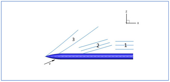
Figure 1.
Sketch of the leeward-side flow regions for a body of revolution.
This paper presents results of the fineness-ratio effects in the flow structure of an ogive-cylinder configuration of L/D = 15, for which abundant experimental and numerical information is available [6,7,13,14,18]. This configuration was tested at Mach number 0.2 and Reynolds number 2 × 10⁶. The experimental data include overall and sectional force coefficients at several angles of attack: 20, 30, 35, 40, 45, 50, 55, and 60 degrees.
This paper also shows results for two other configurations with the same ogival section of the reference geometry: the cylindrical section was varied to yield a short configuration (L/D = 7.5) and a long one (L/D = 30), which should display the three regions, according to Ramberg (L/D > 20). Section 2 gives information on the reference geometry, Section 3 details the numerical procedures and Section 4 studies the effect of the fineness ratio in the overall forces. A detailed analysis of the solutions and flow structure for each configuration comprises the body of Section 5. Finally, Section 6 reports the main conclusions reached in this work.
2. Reference Case: Ogive-Cylinder with Fineness Ratio of 15
The configuration taken as reference for the numerical results is an ogive-cylinder tested by ONERA (Office National d’Etudes et de Recherches Aérospatiales) [6,14,18]. This model was used for studies under an action Group (AG04) of the Group for Aeronautical Research and Technology in Europe (GARTEUR). The test model consists of a 120 mm diameter cylindrical body with a three-caliber tangent ogive nose. The total length is 15 calibers (L/D = 15). This ogive-cylinder configuration was tested in the ONERA F1 pressurized wind tunnel at Le Fauge-Mauzac (France). For the numerical study, the flow conditions were Mach number Ma = 0.20, Reynolds number Re = 2.2 × 10⁶ and angle of attack α = 45.00 degrees. The flow is assumed to be fully turbulent.
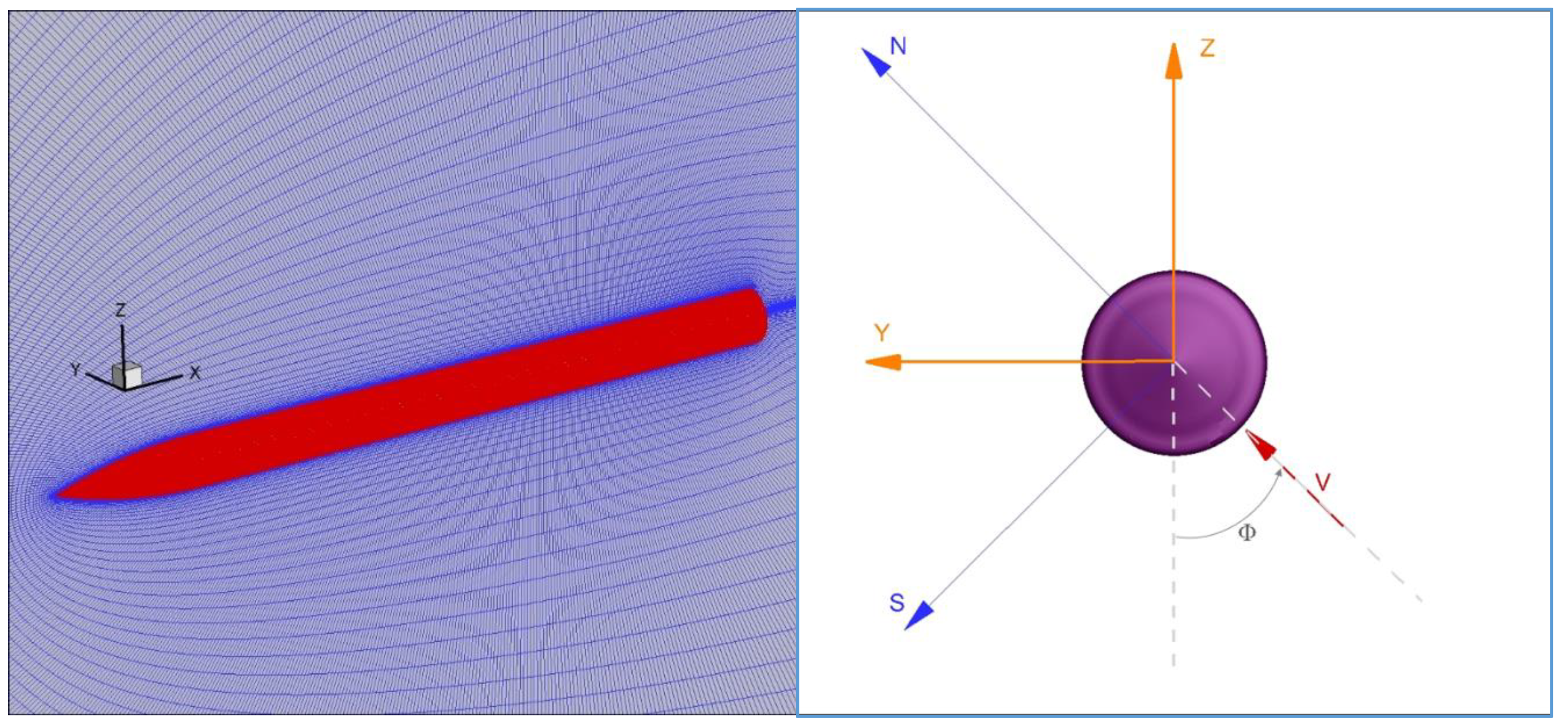
The diameter of the configuration under study was 1 m, the temperature of the air was 288 K, and the pressure and density were adjusted to obtain a Reynolds number similar to that of the experiment. We use a non-rolled axis system. The longitudinal axis is in the x-direction. Figure 2 (left) shows a detail of the mesh at the plane of symmetry y = 0, indicating the Cartesian reference system used, with the origin at the nose. In the right part of Figure 2, the transversal plane y-z is shown, with the roll angle measured at the windward side in a counterclockwise direction. In this axis system, the velocity components are: , being the magnitude of the free stream velocity and the angle of attack.

Figure 2.
(Left): Detail of the mesh at the plane of symmetry Y = 0 with the axis system. (Right): Cartesian reference system based on the roll angle.
The relationship between the coefficients obtained at this non-rolled system with the longitudinal (l), lateral (side) and normal force coefficients is the following:
The calculations shown in this paper are all referred to for a structured grid. It was demonstrated that there were two possible solutions, one mirror of the other, at large angles of attack [13].
3. Numerical Simulation
The numerical study employed the ANSYS FLUENT© code [5], performing URANS calculations with Reynolds Stress turbulence models combined with Scale-Adaptive Simulation (RSM-SAS). For Scale Resolving Simulation (SRS) -which includes LES or RSM-SAS simulations- second order accurate bounded central differencing discretization scheme is used for the momentum equations. A central differencing scheme calculates the face value of a variable as follows [5]: where the indices 0 and 1 refer to the cells that share the face and and are the reconstructed gradients at the respective cells, and the vector is directed from the cell centroid to the face centroid. This scheme can produce unbounded solutions and non-physical wiggles. Therefore, a bounded central differencing scheme is used. This scheme is composed of a pure central differencing scheme, a blending of a central differencing and an upwind scheme, and the upwind scheme [5].
As it was checked after analyzing different CFD solutions from different codes compared to the experimental data [14], the unsteady and asymmetric nature of the flow was not captured with most of the URANS codes used. Only high-level codes using LES or DES approximation could capture the damping of forces at the rear and the unsteadiness. At a high angle of attack of 45 degrees, one-equation turbulence models such as the Spalart-Allmaras model, were not capable of achieving asymmetric flow solutions. This led us to use the most advanced turbulence model available, i.e., the RSM-SAS model. As stated in the Introduction to the paper, details of the RSM-SAS turbulence model can be found in references [1,2,3,4,5].
Structured axisymmetric grids were generated by rotating and replicating every 1.5 degrees a two-dimensional grid. The number of surface elements for the reference configuration (of length 15D) was 78,720, and the total number of cells was approximately 15 million: 450 × 240 × 140 cells in axial, circumferential and radial directions, respectively. The infinite is a cylinder of length 225 D. The origin of the axis system is at the nose, being the free stream upwards at −75 D and the infinite downwards at 150 D. The diameter of the cylinder is 50 D. Non-reflecting boundary conditions are imposed at the infinite. The height of the first cell relative to the body surface was 10−5. With this value, the y+ was about 1 in the whole-body domain. More than 20 cells were within the boundary layer.
3.1. Time Accurate Calculations
It is necessary to perform time-accurate calculations. A second-order dual-time stepping method is implemented into the code in order to make these computations.
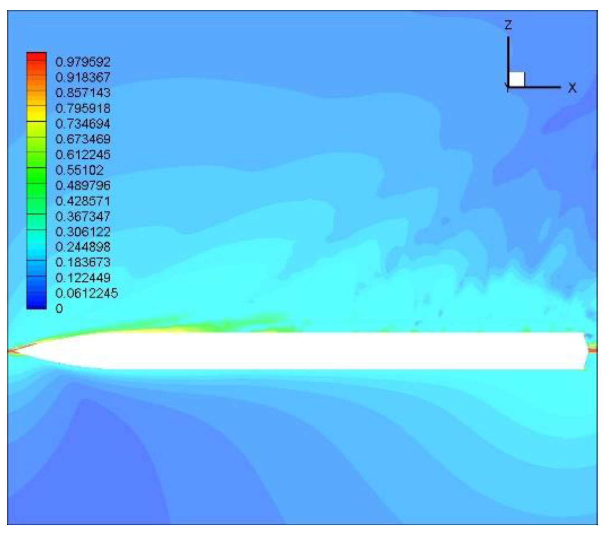
The convective time is . It is also worth using the convective time for crossflow: . For the time step , typical values for obtaining low Courant numbers are to use: [1]. For this case, a value of may be sufficient. A preliminary study with several time steps, ranging from s to s, checked that the largest value was not sufficient due to large oscillations in the forces and large values of the convective Courant number (CFL) in zones of interest. The oscillations damped when using s. Most solutions were obtained with this time step, which is approximately , i.e., being the non-dimensional time . Additional calculations were made using the lowest value s, i.e., . This is a very low value. Figure 3 plots the contours of CFL in the plane of symmetry Y = 0 for the reference case, showing values of order 1 or below in the boundary layer zone when using this last time step. For the typical value , the Courant number CFL was about five in the boundary layer zone.

Figure 3.
CFL contours in the plane of symmetry Y = 0 for the reference configuration (Δt = 10−4 s).
As the computational cost was high, a trade-off between computational time and the accuracy of results must be made. Comparisons between solutions obtained with the two lower values of the time step were made.
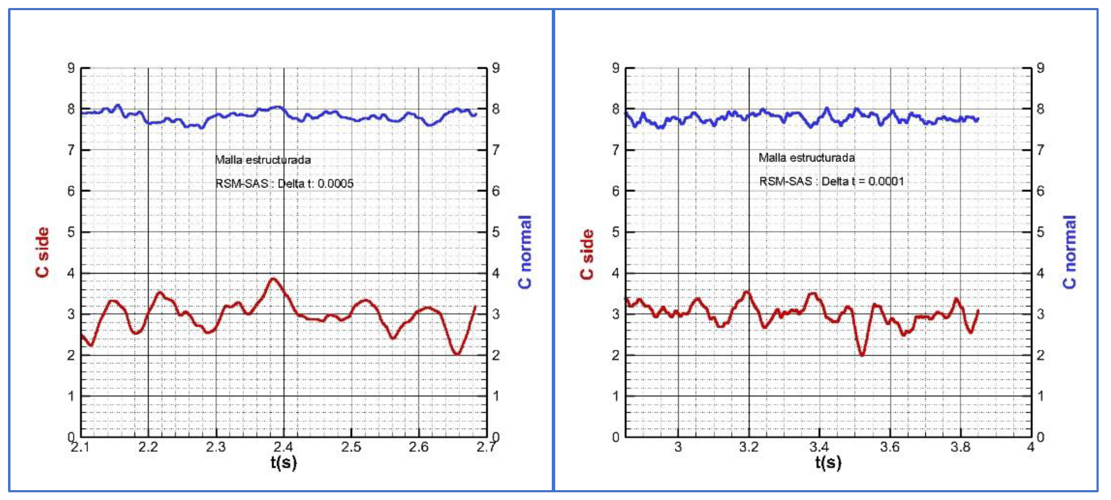
Figure 4 shows the time history for both the side and normal force coefficients of the reference configuration at the flow conditions specified. The average values are very similar, but there are some differences in the power spectral density. The unsteady nature of the flow is captured with both time steps. The solutions -in terms of local forces and pressure distributions- compared well with the experimental data, as shown in another paper by the authors [13].

Figure 4.
Time history for the side force (red) and normal force (blue) coefficients. Left: time step Δt = 5 × 10⁻⁴ s. Right: Δt = 10−4 s.
For the purpose of this study, it was considered that the time step is sufficient for capturing the main features of the flow, reducing five times the computational cost compared to the time step .
3.2. Turbulence Model: RSM-SAS
Typical turbulence models implemented in URANS codes do not display the correct spectrum of turbulent scales, as they are overly dissipative [1]. The advantage of SAS (Scale Adaptive Simulation) is that it can resolve the turbulent scales up to the grid size limit. SAS has an LES-like behavior in unstable regions, and it works in RANS mode in stable regions [2]. A good example of the variety of solutions that SAS is capable of achieving, depending on the time resolution and grid size, is given in [3]. Several turbulence models, either eddy-viscosity turbulence models like k-ω SST or Reynolds Stress turbulence models (RSM), were used before RSM-SAS was utilized. The solutions obtained with this turbulence model were quantitatively and qualitatively much better than the others when compared to the experimental data. This is documented in [13]. Therefore, only URANS calculations with RSM-SAS using fine grids and small time steps were done for the study of the influence of body length on instability and flow asymmetry.
3.3. Influence of Roughness: Structured vs. Unstructured Grids
An important question to clarify is the use of structured grids generated in the way explained above. There was no roll angle dependence on the side force magnitude; nevertheless, when using unstructured grids generated with a procedure that included nose irregularities, as well as roughness, the roll angle dependence of the side and normal forces was clearly checked. In order to quantify these differences, a ‘numerical roughness’ is defined in the following manner: First of all, as the test model is a body of revolution, the average radius at each x/D section is defined as:
. Then, the ‘numerical roughness’ at each section is calculated by the following expression:
. The evaluations at different x/D sections of the unstructured grid show results of ‘numerical roughness’ between 40–60 × 10−6 m, i.e., rn/D = 40–60 × 10−6 in the cylindrical part, while larger values were obtained for the ogive. A similar evaluation for the structured grid led to values more than an order of magnitude lower.
We can conclude that the unstructured grid resembles a rough model, while the structured grid resembles a polished model. The results of the different grids—ranging in angle of attack—compared well with the experimental data ([6,14,18]). These comparisons and the conclusions about the influence of the grid in capturing both global instability and convective instability are shown in another paper by the authors [19].
There was no systematic grid convergence study. Several structured grids were used, generated with the same procedure but increasing or reducing the surface mesh density or the volume mesh density in a radial direction. All these meshes resemble polished models, and there was no roll angle dependence on the forces. However, the two possible solutions observed experimentally [6] for the side force were achieved, depending either on the infinite roll angle or on the initial conditions. In order to clarify this point, a plot of the time history of the side force coefficient at two different initial conditions is shown in Figure 5.
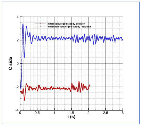
Figure 5.
Convergence history of the side force coefficient for the structured grid (reference configuration) starting with two different initial solutions.
The red line shows the side force coefficient history when starting the time marching procedure using a steady calculation converged solution as the initial flow field. In this case, the sign of the side force is not changed, and the evolution is such that the side force coefficient converges to a fluctuating solution with an average value close to −2.00. The blue line solution is obtained after an unsteady calculation starting with a non-converged steady calculation flow field as the initial solution. In this case, the side force changes its sign from the negative initial solution to a positive final side force. This side force is also fluctuating with a similar dominant frequency, and the average side force coefficient is close to 2.00. Then, the bi-stable pattern shown in several experiments for polished models at high incidence (see [6]) is reproduced numerically. Numerical perturbations at the time marching procedure or a bias in the initial flow field leads to one of the two possible mirror solutions. The flow patterns are similar: an asymmetric flow field with a vortex pair structure such that a vortex on the starboard or port side is dominant.
The use of structured grids is considered to be more useful for the studies of the fineness ratio influence on the flow pattern, as it avoids the effect of adding additional sources of instability to the flow due to the geometrical imperfections, resulting in an uncomfortable roll angle dependence.
The next sections show comparisons with the experimental data of the numerical solutions in terms of pressure coefficient, sectional forces and overall forces. A detailed analysis of the reference configuration (L/D = 15) is given in [13].
4. Effect of the Fineness Ratio on the Overall Forces
In order to study the fineness ratio effect, the 15-caliber reference configuration is modified by shortening and stretching the cylindrical afterbody, yielding two additional configurations of L/D = 7.5 and 30. The same parameters for mesh generation were used for the three configurations so that all the configurations have the same number of grid points in the volume mesh—approximately 15 million cells—and the same number of grid points in the surface mesh. Therefore, the length of the cells in the streamwise direction for the long configuration is twice the length for the reference geometry and four times the length for the short one. In radial and normal directions, the size of the cells is the same for all meshes. Consequently, the short configuration has lower cell aspect ratios than the others near the body.
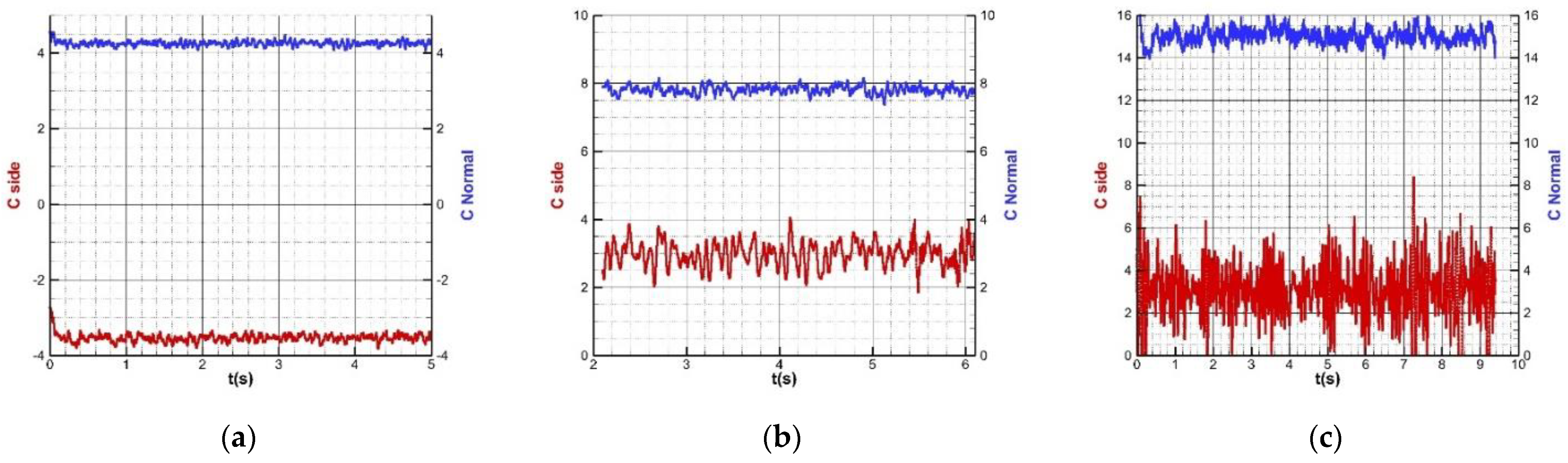
The flow condition is Mach = 0.2, Reynolds number Re = 2 × 10⁶ and angle of attack α = 45 degrees. Most calculations were made with a time step of s. With this time step, 1 s of calculation is achieved after 2000 time steps. The computation is stopped at 5 (10000 Δt), 4 (8000 Δt) and 9.4 (18800 Δt) seconds for fineness ratios of 7.5, 15 and 30, respectively. Figure 6 shows the time histories of the side and normal force coefficients, for which the average () and standard deviation () appear in Table 1. It is important to remark that there is a numerical transient period before the flow becomes fluctuating with some periodicity.
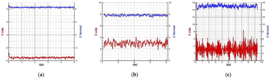
Figure 6.
Time histories of the side and normal force coefficients. (a) Short body; (b) Reference configuration; (c) Long body.

Table 1.
Side and normal force coefficients versus fineness ratio. Ma = 0.2, Re = 2 × 10⁶ and α = 45 degrees.
A first insight in the three curves shows that the oscillations of the coefficients for the short body are very small, leading to a quasi-steady solution. Regarding the reference configuration, the minimum side force coefficient is around two, and the maximum is four over the period analyzed. The standard deviations of the side force coefficient for the long configuration are very large. There are values of the coefficient reaching eight, while the average in the period is around three. Champigny [6] describes a linear correlation between the angle of attack for the onset of asymmetry and the nose angle for pointed ogives or cones. For the ogive of our configuration, this angle of onset is However, the effect of fineness ratio was also relevant, and this angle is reduced due to the cylinder: the slenderer the body, the lower the onset angle. The calculations were made at an angle of attack of 45 degrees, far from the onset angle for the three configurations, so there is a net side force for all the configurations.
The fineness ratio has a predominant effect on the unsteadiness of the flow. The flow may become asymmetric from the tip due to the hydrodynamic instability mechanism described by several authors ([6,8,9]). Region 3 is essentially steady. Figure 6a indicates that this zone is predominant in the short body, leading to small oscillations of the forces. Region 2 introduces a certain degree of unsteadiness due to oscillations of the strength and position of the vortices and the shear layers, increasing the amplitude of the force oscillations for the reference geometry (Figure 6b). The appearance of Region 1, where the vortices shift from one side to the other in a Karman vortex fashion, leads to the largest standard deviation for the long body (Figure 6c). The analysis of the sectional forces below will support this rationale. There is a study of a similar configuration at low subsonic flow and low Reynolds number with fineness ratios 10, 15 and 20, which support this idea of increasing instability and unsteadiness with the fineness ratio. At the same angle of attack, the Strouhal number is zero for the short configuration while approaching 0.175 for the long configuration [20].
5. Analysis of the Sectional Forces and the Flow Structure
- A.
- Configuration with Fineness Ratio L/D = 7.5
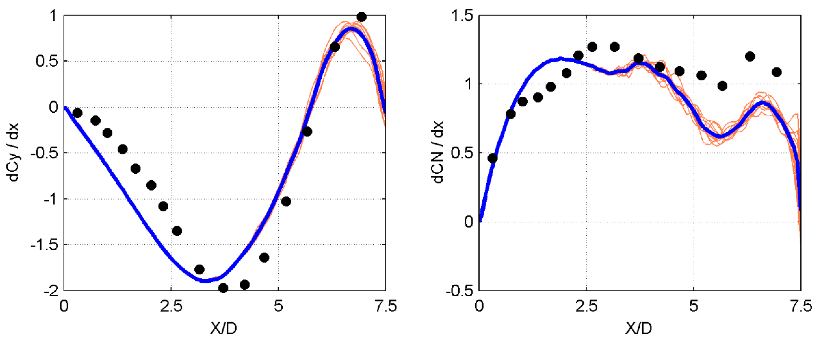
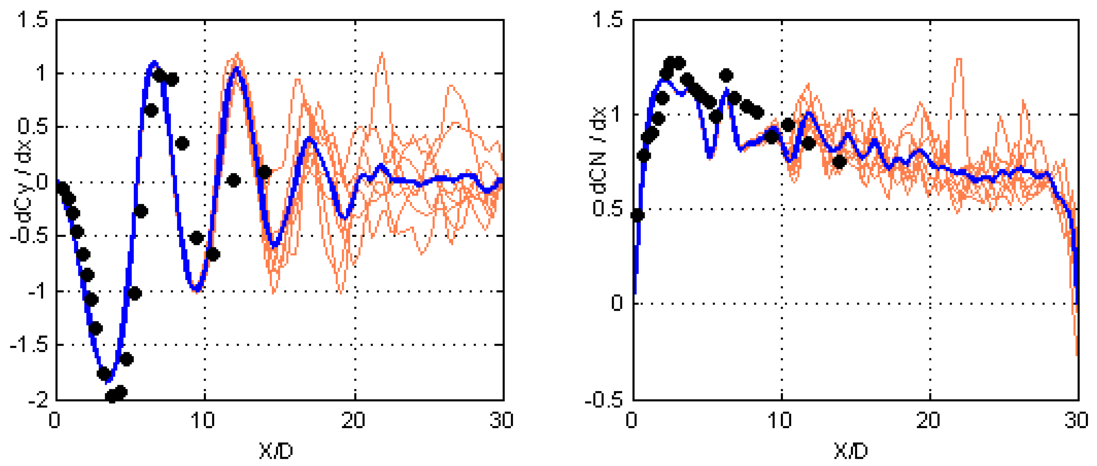
Figure 7 plots with orange lines instantaneous sectional force coefficients for 20 instants chosen within the last 0.5 s of the calculation, for which the overall forces are represented in Figure 6a. The thick blue line represents the discrete average curve, and the solid black circles are the experimental sectional force coefficients for the reference configuration of the fineness ratio of L/D = 15. From the visibility of the orange lines, we can conclude that Region 3 extends approximately up to x/D ~ 5. The rest of the body corresponds to Region 2, being responsible for the small oscillations that appear in Figure 6a. The averaged side force reaches maxima or minima at x/D ≈ 0, 3.3 and 6.7.

Figure 7.
Instantaneous and average sectional forces (short configuration).
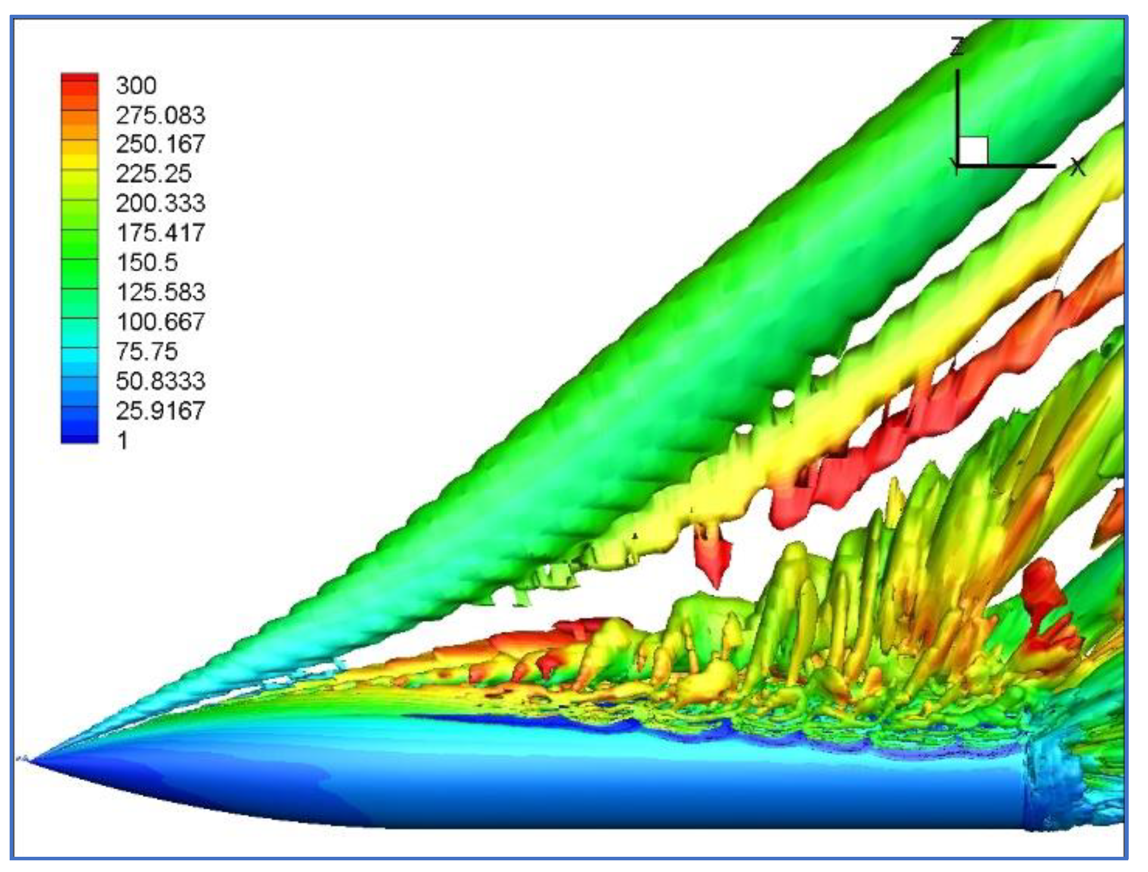
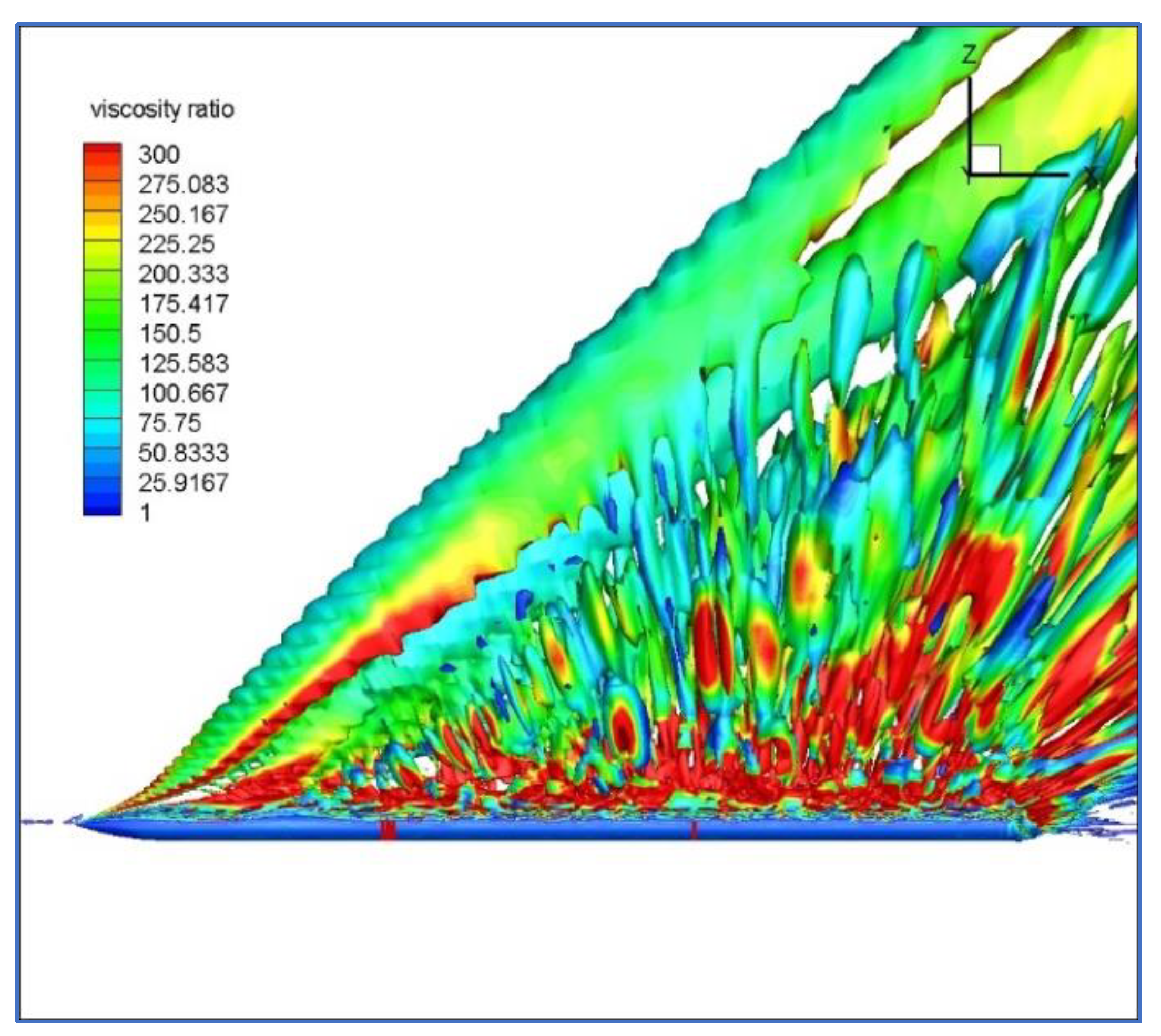
Figure 8 shows iso-Q contours, colored with viscosity ratio , computed at the last moment of the calculated period (t = 5 s). Q is the second invariant of the velocity gradient tensor: where ω is the norm of the vorticity tensor, and S is the norm of the strain rate tensor [21]. These iso-Q contours help to identify coherent vortex structures. The first maximum of side force occurs at x/D = 3.3 (see Figure 7), while the main vortex sheds between sections x/D = 4.5 and x/D = 4.75.

Figure 8.
Positive iso-Q contours (short configuration) colored with viscosity ratio.
The solution is consistent with the analysis of Degani et al. [16]: Region 3 is dominant, and Region 1 is virtually nonexistent for bodies with a lower fineness ratio (L/D < 16). There exists an effect of the base flow and an incipient Region 2, but the fluctuations of the flow are very small, leading to a practically stationary flow, as can be checked in the time history of the overall forces (see Figure 6).
- B.
- Configuration with Fineness Ratio L/D = 15
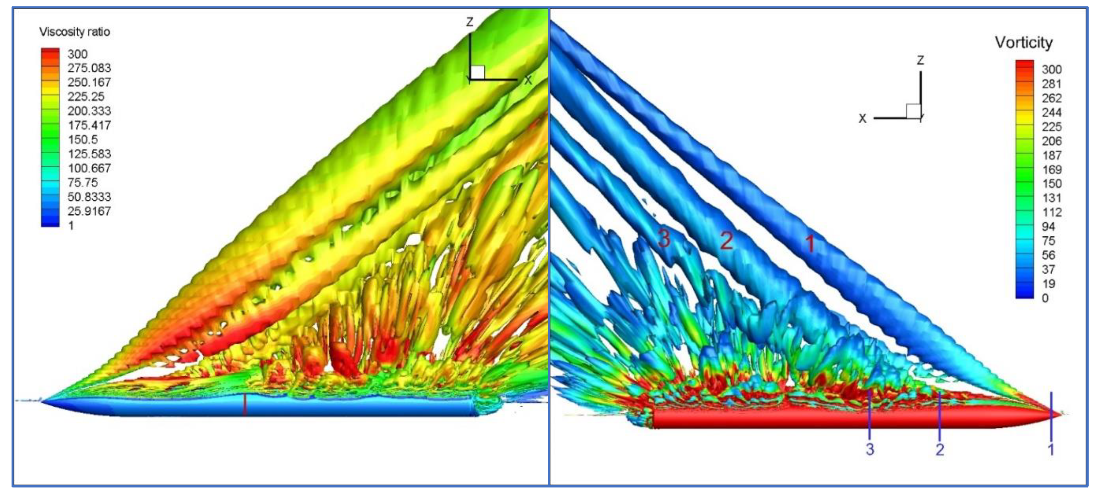
For the reference configuration of the fineness ratio of L/D = 15, an unsteady solution obtained over 2.1 s with the RSM model was used as the initial solution. The calculation was then resumed using the RSM-SAS model, computing four additional seconds. The solutions of the sectional side and normal force coefficients for several points in time over the last 0.1 s of the interval are shown in Figure 9 (20 solutions taken at each time step s). In this case, these two regions are clearly differentiated. Up to x/D ~ 7.0, all solutions coalesce (Region 3). In the rear part, the multiple lines indicate the unsteadiness of the flow (Region 2). Iso-surfaces of positive Q-function (up to 5000) are shown in Figure 10 for the time t = 6.1 s. They are colored with the viscosity ratio magnitude (left) and vorticity (right).
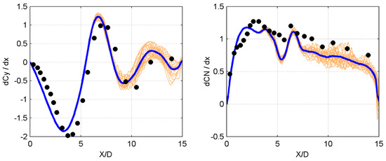
Figure 9.
Instantaneous and average sectional forces (reference configuration).

Figure 10.
Positive iso-Q contours (reference configuration). (Left): colored with viscosity ratio. (Right): colored with vorticity.
The flow structure of the short configuration shown previously is similar to that of this reference configuration, as can be seen by comparing Figure 8 and Figure 10. The main difference lies in the length of Region 2, which is very small for the short configuration. The first maximum of side force occurs at the same location for both configurations, i.e., x/D = 3.3. The main vortex sheds in a similar location as that of the short configuration. In general, the flow structures of both configurations are similar up to x/D ≈ 7 (see Figure 7 and Figure 9), showing that the nose effect is dominant.
The red line marked in the body of Figure 10 (left) shows approximately the transition between Regions 2 and 3. This corresponds to x/D ~ 7. There is a continuous vortex structure in the steady region, while the flow breaks into different scales in Region 2.
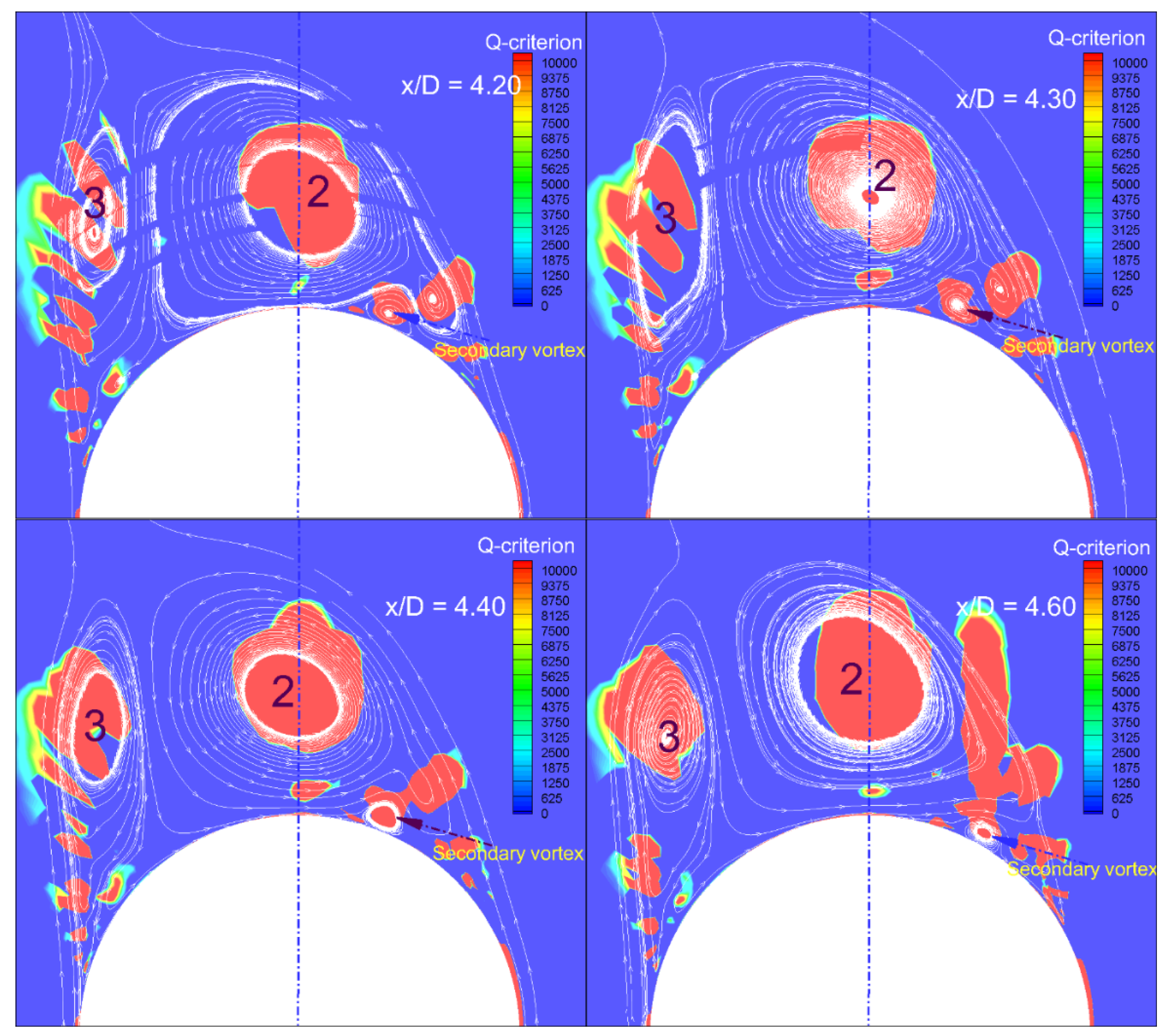
The blue marks with symbols ‘1, 2, and 3’ in the right figure (Figure 10) indicate the approximate location of vortex shedding at the stationary region (Region 3), which does not correspond exactly with the maximum or minimum of the local side force coefficient. The minima or maxima (averaged side force coefficient) are located at x/D = 0.0, 3.33, 6.67, 9.24, 11.97 and 14. 1 (see Figure 9). The vortex labeled 1 (Figure 10) sheds at the nose approximately. However, the vortex labeled ‘2’ is shed at x/D = 4.50 approximately. This can be explained by looking at Figure 11, which shows the pseudo-streamlines at four longitudinal sections and the Q-function contours taken at one of the 20 solutions analyzed. At this region, the flow is steady (see Figure 9). At section x/D = 3.30 (local minimum of side force coefficient), the vortex labeled ‘2’ is attached, and its center is located at leeside and close to the y = 0 plane. There is an incipient vortex 3 attached at the starboard side but of lower strength. This balance leads to a maximum side force magnitude. This pair of vortices develop such that vortex 3 increases its strength while vortex 2 reduces it, thus contributing to reducing the side force; at section x/D = 4.30, vortex 3 is attached, and vortex 2 core is located at the plane of symmetry. In section x/D = 4.40, there is flow entrainment in vortex 2 from vortex 3. At section x/D = 4.50, vortex 2 is detached. The shedding occurs closer.

Figure 11.
Contours of positive Q criterion (reference configuration) and pseudo-streamlines at four sections.
A similar pattern is reproduced with vortex 3 and a new one labeled ‘4’, leading to a vortex shedding at x/D = 6.67, which coincides approximately with another peak in the local side force coefficient. After this, from x/D = 7.0 on, there is an unsteady flow, and the flow breaks into several turbulent scales.
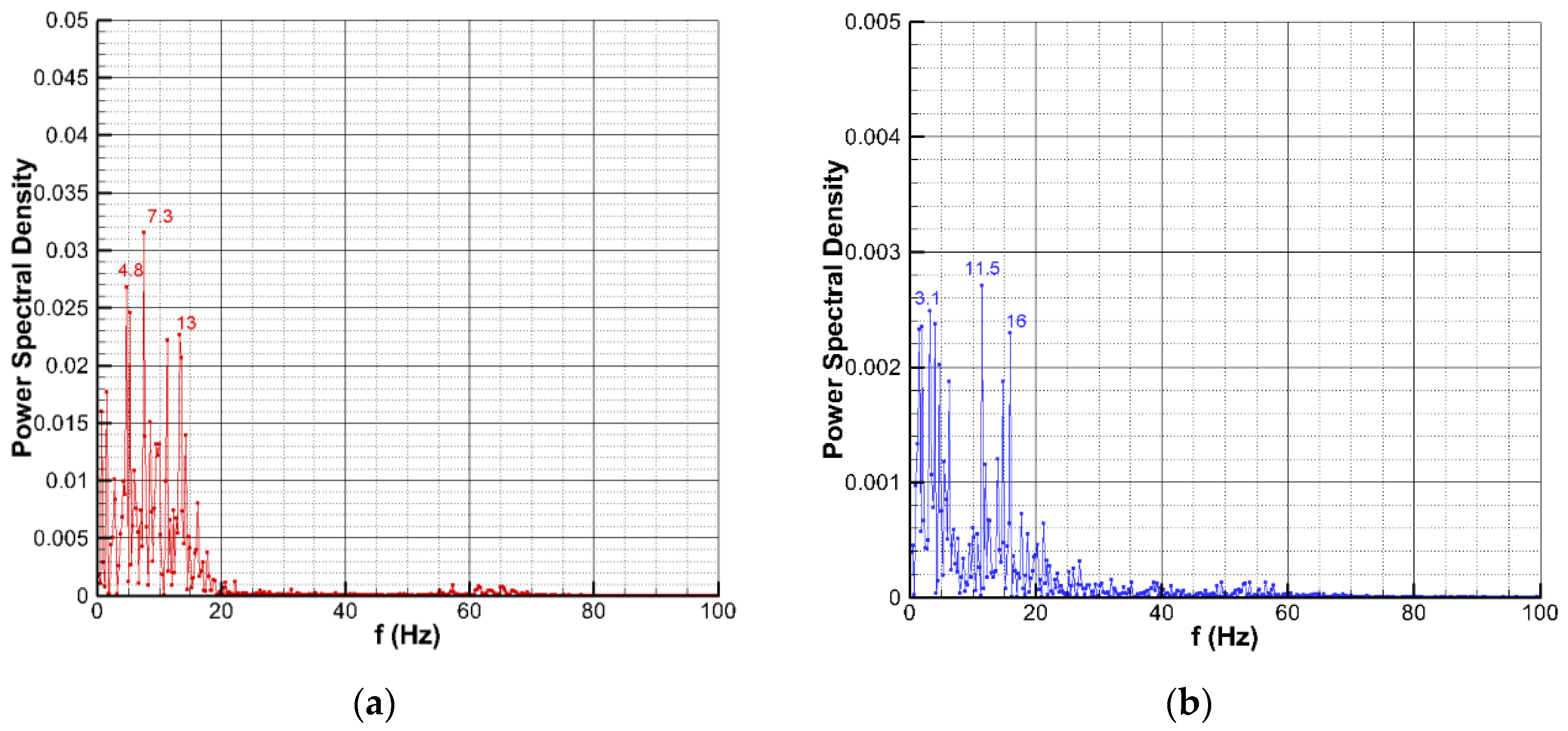
The Power Spectral Density (PSD) of the side and normal forces for the interval t = 2.1–6.1 s are shown in Figure 12. There is a small content of energy above 20 Hz. The characteristic crossflow time and Strouhal number of the von Karman street are: .

Figure 12.
PSD of the side and normal force coefficients (reference configuration). (a) Side force coefficient; (b) Normal force coefficient.
The theoretical value St = 0.2, characteristic of the infinite cylinder in crossflow, yields a frequency of 9.6 Hz, not concordant with the dominant frequency of 7.3 Hz in this calculation, which corresponds to a Strouhal of 0.15. It is worth noting that the experimental Strouhal for this configuration was 0.16, in accordance with the results by Prananta et al. [14]. For the short configuration, there was no power spectral density analysis, as the flow was basically steady on the entire body.
Some other frequencies also display a significant content of energy. It is important to remark that for the correct prediction of the low-frequency part of the spectra of the forces it is needed a long physical time integration [22]. For this reference configuration, the time integration was t = 4 s (8000 Δt). The dominant frequency is in accordance with the experimental Strouhal referred to in reference [14], but this lower frequency of 4.8 Hz may be somewhat amplified for numerical reasons. Regarding the normal force coefficient, the amplitudes of the normal force oscillations are an order of magnitude lower. There are two dominant frequencies (11.5 and 16 Hz). It is important to remark that the normal force is independent of whether the vortex asymmetry is left or right-handed [9]. The double frequency of the dominant frequency for the side force is 14.6 Hz, which lies between these two frequencies. The lower frequency with energy content is 3.1 Hz, similar to that of 2.8 Hz for the side force coefficient.
A deeper insight making a longer physical time integration to compare to the actual results is necessary to analyze the origin of this content of energy at those lower frequencies correctly.
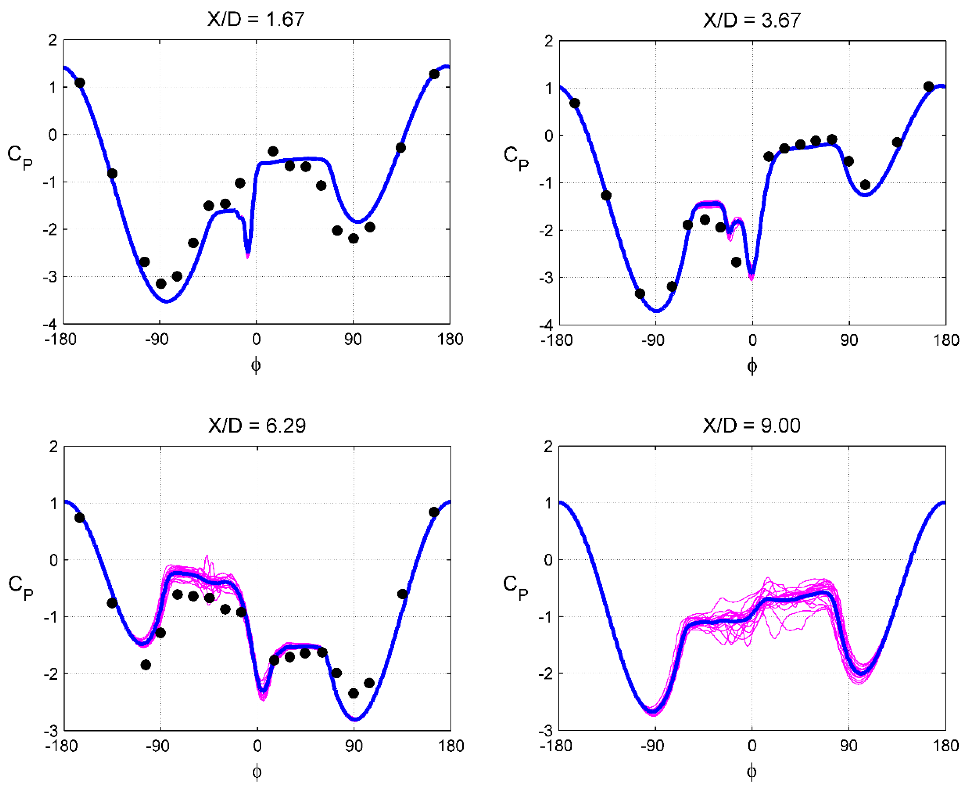
In the test model, there were pressure data taken in several sections. Based on the crossflow dynamic pressure, we define the following pressure coefficient: .
Figure 13 plots the solutions of pressure coefficients in a circumferential direction for 20 instants over the last 0.1 s (magenta lines), together with the average values (blue lines) and the available experimental data (black dots). The figure includes four cross-sections. There is no available experimental information for the last section. It is important to remark that for this comparison, the origin (Φ = 0) of the roll angle corresponds to the leeside. Positive values denote locations at the starboard side, while negative Φ values represent the portside. The first and second sections (x/D = 1.67 and 3.67) are located in Region 3 of the flow. The third section (x/D = 6.29) is located just in the transition between Regions 2 and 3; it corresponds approximately to the maximum side force location: x/D = 6.7 (see Figure 9). The flow in the leeside is slightly fluctuating. These fluctuations significantly increase at x/D = 9 (Region 2). Note the oscillation of the minimum pressure values. The unbalance of all the curves on the same side indicates that there is no alternate shedding.

Figure 13.
Instantaneous and average pressure coefficient in a circumferential direction at four cross sections (reference configuration).
The unsteadiness of the flow is located at the ogive and fore cylinder (up to x/D = 7.0), as shown by the force coefficients curves (Figure 9), iso-Q contours (Figure 10) and pressure coefficients (Figure 13). Then, the oscillations occur at this part, although the different body parts have not been analyzed separately. In the very good detailed work shown in reference [20] it is shown the time histories for the side force coefficients of the ogive and cylinder of a body of fineness ratio of L/D = 20. It is clear that the flow is steady in the nose region, while there is a fluctuating flow with a Strouhal number of St = 0.15 approximately. Although this calculation is done at laminar flow conditions (low Reynolds), this Strouhal is close to the value obtained for this configuration of lower fineness ratio (L/D = 15) at the same Mach number but at turbulent flow conditions.
The good comparison with experiments both in local sectional forces and pressures (see Figure 9 and Figure 13) indicates that the flow field structure shown in Figure 10 with two differentiating regions—one steady in the forebody and one unsteady in the rear cylinder part—approximates to the real flow field close to the body at high incidence. The contours of the Q-function, together with the pseudo-streamlines of Figure 11, help to identify the vortex structure and the alternating vortex shedding. A detailed explanation of this vortex structure in the forebody region is given in [13].
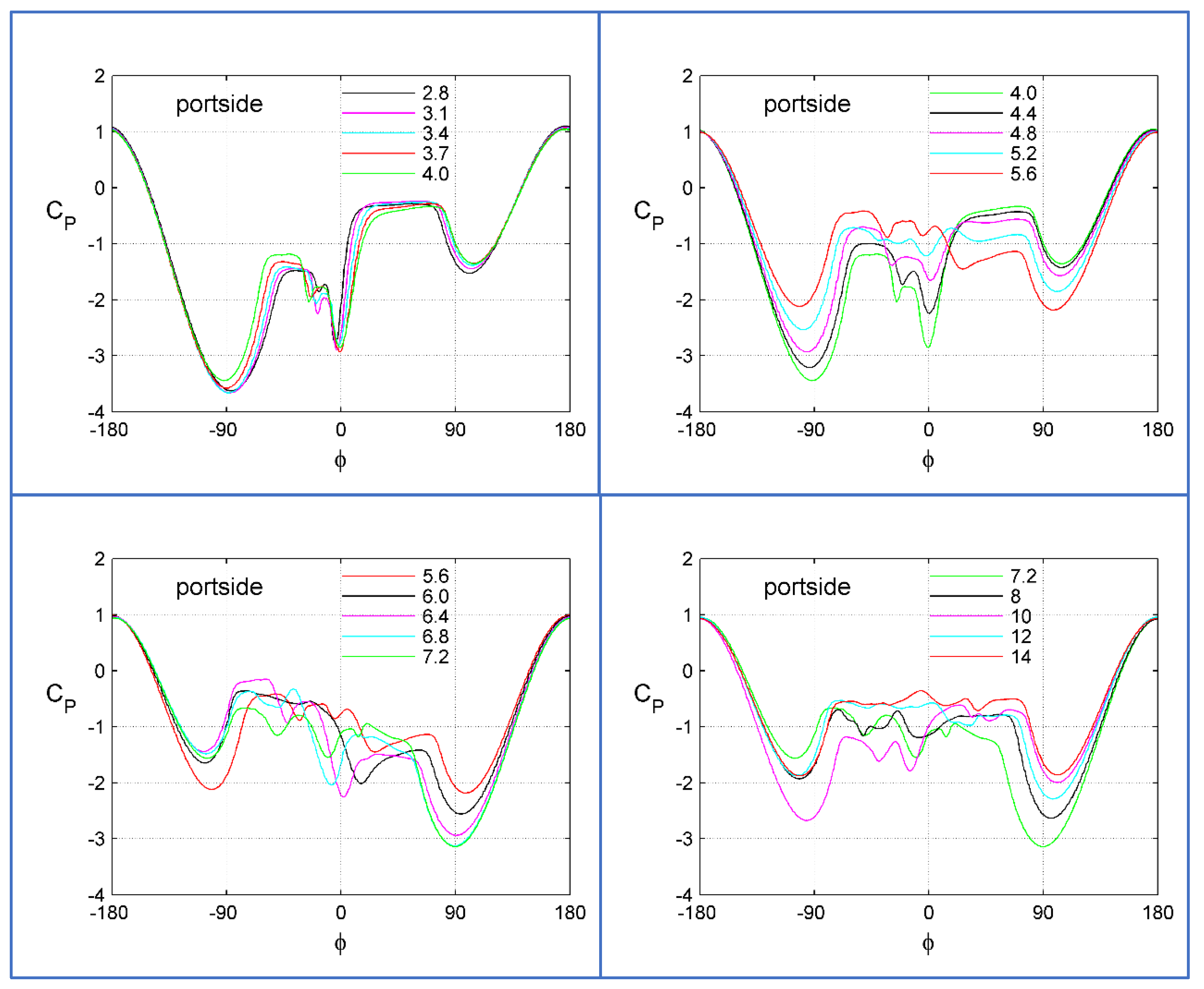
This type of diagram, together with the averaged pressure coefficients at different sectional cross-sections, permits the study of the vortex structure. Figure 14 plots the solutions of the averaged pressure coefficients in a circumferential direction at several cross-sections over the last 0.1 s.
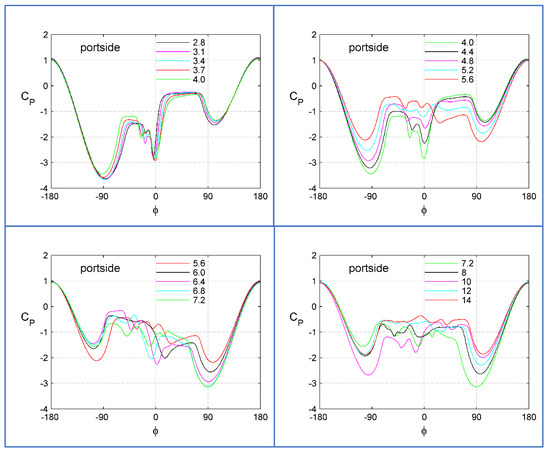
Figure 14.
Average pressure coefficient in a circumferential direction at different cross sections (reference configuration).
The pressure coefficients at x/D = 2.8 to 4.0 are shown in the top left part of the Figure. They indicate a similar flow structure in this region, covering the ogive part of the body. The vortex core is located in the plane of symmetry at leeside, yielding a peak of suction at roll angle Φ = 0 deg. (measured from the top) whereas the port side separation line moves towards Φ = −90 deg. The presence of a secondary vortex is visible in the pressure coefficient at the port side. The minimum side force coefficient location is close to x/D = 3.2. It is worth noting that the main contribution to the side force comes from the attached flow region [23]. In this section, the difference in minimum pressure coefficient between the port and starboard sides reaches its maximum. There is a dominant vortex 2 and an incipient counter-rotating vortex 3. The top right figure shows the pressure coefficients at cross sections x/D = 4.0 to 5.6. As shown in Figure 11, at section x/D = 4.20 (between 4.00 and 4.4 of the figure), there is flow entrainment from vortex 3 to vortex 2. It can be seen that at region x/D = 4.4, the suction peak is reduced, leading to an increment of the minimum pressure at the leeside (Φ = 0 deg.), and the vortex 2 is detached at section x/D = 4.6. Between sections x/D = 5.2 and 5.6, vortex 2 is shed while vortex 3 evolves increasing its strength and moving its center towards the plane of symmetry at leeside (Φ = 0 deg., plane y = 0). The pressure coefficient at section x/D = 5.6 shows, as a result, a lateral force that decreases as the differences between minimum pressures at the port and starboard sides (close to Φ = −90 deg. and Φ = 90 deg.) are reduced significantly compared to that of section x/D = 3.2. The pressure coefficients shown in the bottom left figure (Figure 14) are those corresponding to the cross sections x/D = 5.6 to 7.2. The change to positive side forces and to the transition to the unsteady flow region is shown in these plots. There is a dominant vortex 3 at the port side and an increasing strength vortex 4 at the starboard side, leading to a maximum side force between x/D = 6.6 and 7.2 (close to x/D = 7.0). In this section, the maximum difference in minimum pressure coefficients close to the separation lines (around Φ = −90 and Φ = 90 deg.) is produced.
The pressure coefficients shown in the bottom right of Figure 14 are those corresponding to the cross sections x/D = 7.2 to 14. They show a more complex pattern, leading to a single plateau in the average pressure coefficient at leeside. This is similar to the pressure coefficient of the infinite circular cylinder at crossflow. The flow structure becomes very complex and unsteady. The Strouhal number for this configuration at incidence is St = 0.15. The contribution comes from this rear part of the cylinder.
Finally, we have analyzed the separation and attachment lines for this configuration and reference case [23]. The information for 20 instants over the last 0.1 s is utilized. In a body at incidence, two main zones can be distinguished at a cross-section. On the windward, the boundary layer is attached. On the leeside, primary and secondary separations give rise to a complex flow field. This can be seen in Figure 15 (left) at cross-section x/D = 3.67. The pressure contours and the pseudo streamlines are plotted. The attachment point is defined as the minimum velocity point, while the separation points are those where the boundary layer separates. In the figure, the angles Φ1 and Φ2 define the location in a circumferential direction of these points, one located at the port side and another at the starboard side. It has been checked in Figure 14 that the attachment points are located close to Φ = 90 or Φ = −90 deg., according to the definition used for the pressure coefficient (Φ = 0 located at the leeside in the plane y = 0). It is interesting to calculate the attachment line location for the whole body and also the separations lines. The separation lines are calculated with the criterion of minimum shear stress magnitude, being this magnitude . A plot of the separation lines (red color and left scale) together with the attachment line (blue color and right scale) is shown on the right side of Figure 15. It is important to remark that for this figure, the origin of the angle is at the windward side (as seen in Figure 15). An additional green line curve represents (units in degrees). This curve represents the difference between the separation points on the port and starboard sides. This is an indicator of the level of asymmetry in each section. This way, indicates symmetric separation points. The main conclusion obtained by looking at the figure is that the curves follow the same trend as the sectional side force coefficient curve (see Figure 9). However, the attachment line evolves in an opposite phase. A clockwise turn of the separation points is accompanied by a counterclockwise movement of the attachment point. The flow passing through the starboard side feeds the strong central vortex: a low-pressure region compared to the port side values. As a consequence, a greater volume of the incoming flow is forced to pass through starboards, shifting the attachment point to the starboard side. In the unsteady region (X/D > 7.00), both the separation and the attachment lines tend to be symmetric scenarios in accordance with the decay of the cross-sectional side force amplitude. It is also worth noting that the attachment line is offset at x = 0 (about 1.5 deg. to the port side), which is an indicator that the flow is asymmetric from the nose (steady region) and then oscillates around this biased value. It is worth noting that at x/D = 7.0 approximately, both the attachment and separation lines are thicker lines, showing the fluctuation of the attachment and separation points at the cross sections of this rear zone. The unsteadiness of the flow is reflected by the fluctuation of these lines, which is greater as one moves toward the base region. This is another way of measuring and defining the unsteady flow Region 2.
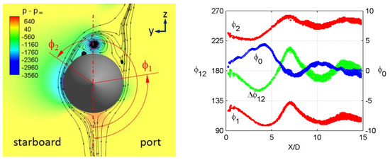
Figure 15.
(Left): Pressure contours and pseudo streamlines at x/D = 3.67 (reference configuration). (Right): Separation and attachment lines.
- C.
- Configuration with fineness ratio L/D = 30
The time history of the overall force coefficients for the long configuration can be seen in Figure 6c. The period is 9.4 s. The averaged values and standard deviations are printed in Table 1. Figure 16 plots the sectional side and normal force coefficients for 20 instants, taken each s, over a period of 0.1 s of calculation. As before, the blue line represents the discrete average values and the solid black circles, the experimental sectional force coefficients for the reference configuration. The numerical values in the ogive are similar to the experimental data of the reference configuration, indicating a small influence of the base flow in the nose. The steady zone stretches up to x/D ~ 11. Recall that this value was x/D ~ 6.5–7 for the reference configuration.

Figure 16.
Instantaneous and average sectional forces (long configuration).
The averaged side force reaches maxima or minima at x/D ≈ 0, 3.3, 6.7, 9.4, 12.1, 14.6, 17 and 19.4 (see Figure 16). After x/D = 20, it remains near zero, while the instantaneous force displays alternating positive and negative signs, the expected behavior of the vortex Karman street (Region 1). Thus, the three regions identified by Ramberg [15] and Degani et al. [16,17] are visible in Figure 16: Region 3 extends from the nose up to x/D = 11, approximately; Region 2, from x/D = 10 to 20, and Region 1, from x/D = 20 to the base.
Iso-surfaces of positive Q-function (up to 5000) are shown in Figure 17 for the time t = 9 s. They are colored with the viscosity ratio magnitude.

Figure 17.
Positive iso-Q contours (long configuration) colored with viscosity ratio.
The red lines marked in the body of Figure 17 show approximately the transition between Regions 1 and 2 and Regions 2 and 3. This corresponds to x/D ~ 20 and x/D ~ 10 respectively. There is a continuous vortex structure in the steady region, while the flow breaks into different scales in Regions 1 and 2.
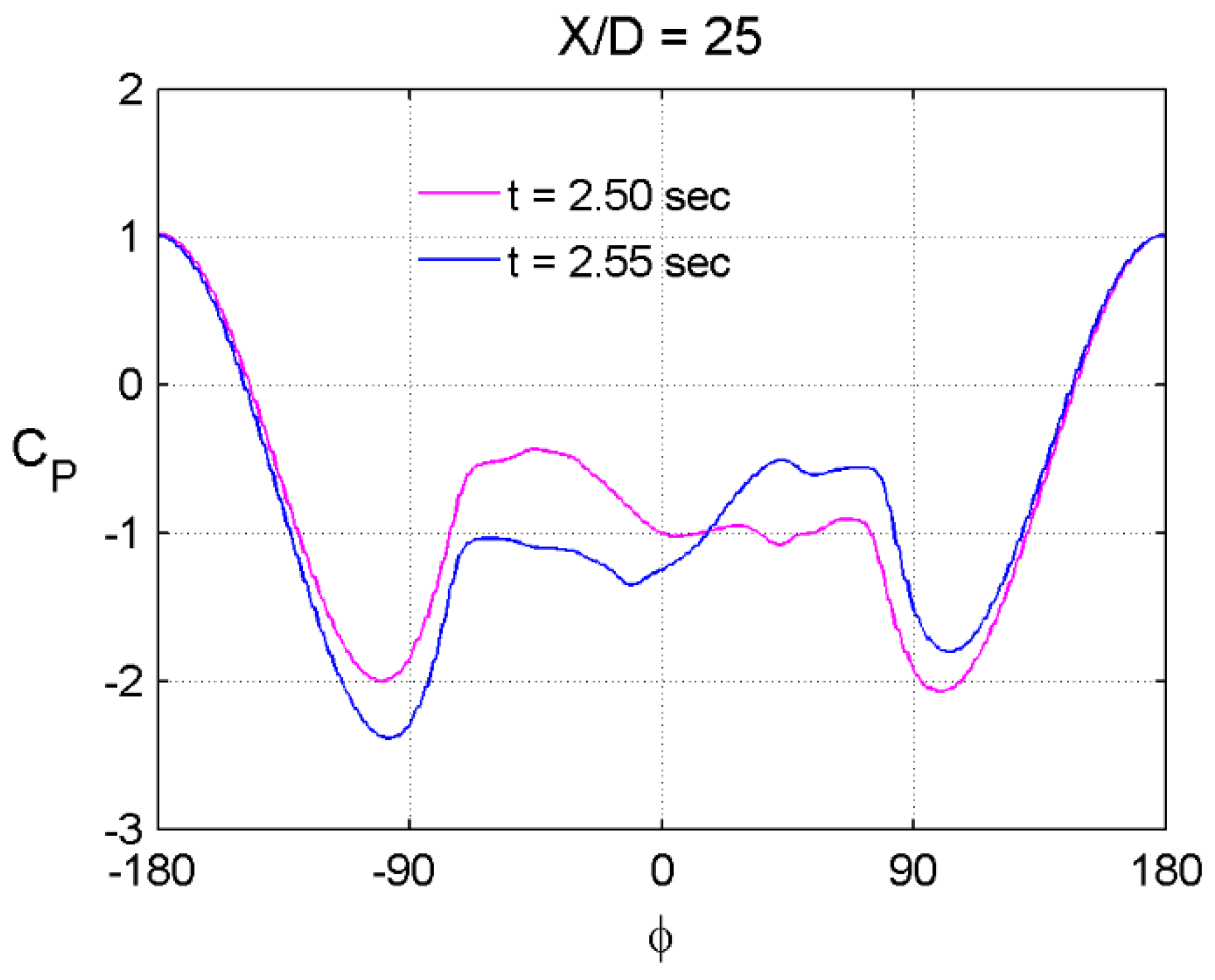
We can also appreciate the effect of the von Karman vortex street by looking at the pressure distributions along crossflow sections. Figure 18 plots the pressure coefficient at a rear section at two points in time approximately half a cycle apart. The pressure at t = 2.55 s changes its pattern with respect to the pressure at t = 2.50 s. During this interval, the minimum pressure induced by the dominant vortex shifts from the port side to the starboard side.
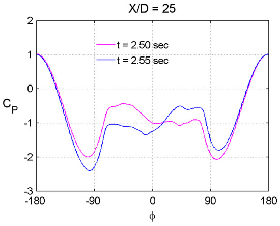
Figure 18.
Pressure coefficient at two moments in cross-section x/D = 25 (long configuration).
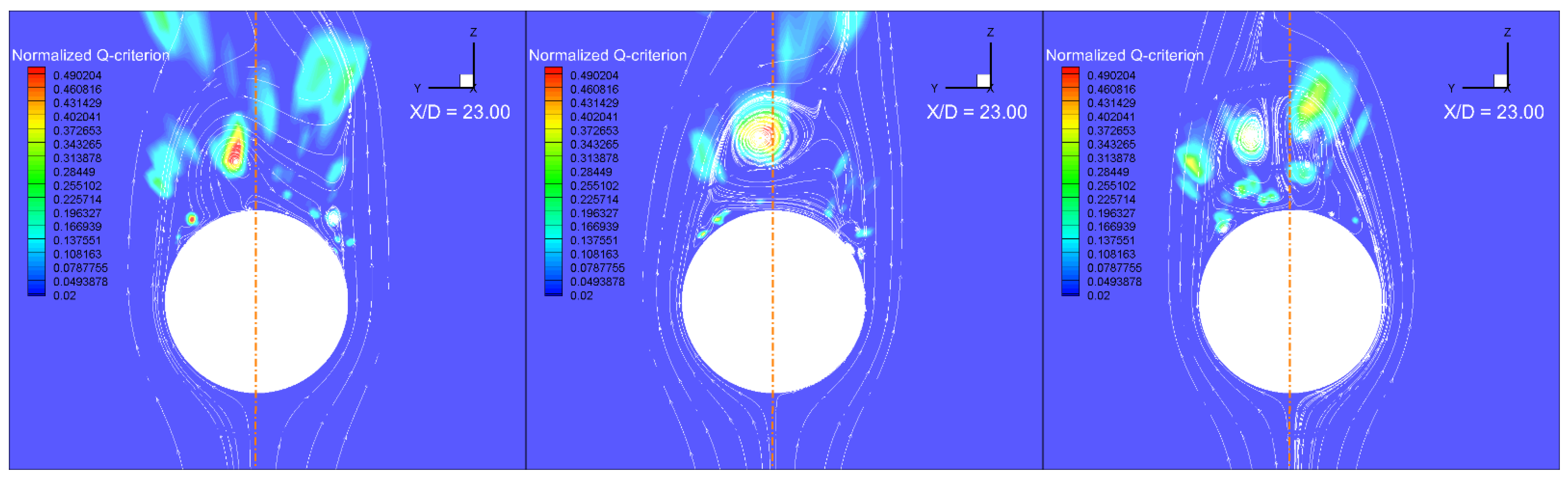
Figure 19 shows the normalized Q-criterion and pseudo-streamlines at section x/D = 23.0 (rear body, flow Region 1), in which the flow has a similar behavior to that of section x/D = 25.0. These plots correspond to three different times (t = 2.505, 2555, and 2.605 s) within a period of 0.1 s again. There is a complex vortex structure with vortices of different scales. The nature of the fluctuating flow leading to a zero net side force within the period is shown here. However, the differences between the contours at t = 2.60 s (right side of the figure) compared to t = 2.505 s (left side of the figure) indicate the complexity of the flow at the rear part of the body.

Figure 19.
Positive normalized Q-criterion contours (long configuration) and pseudo-streamlines at cross-section x/D = 23.0 and three different instants (Left): t= 2.505 s. (Center): t = 2.555 s. (Right): t = 2.605 s.
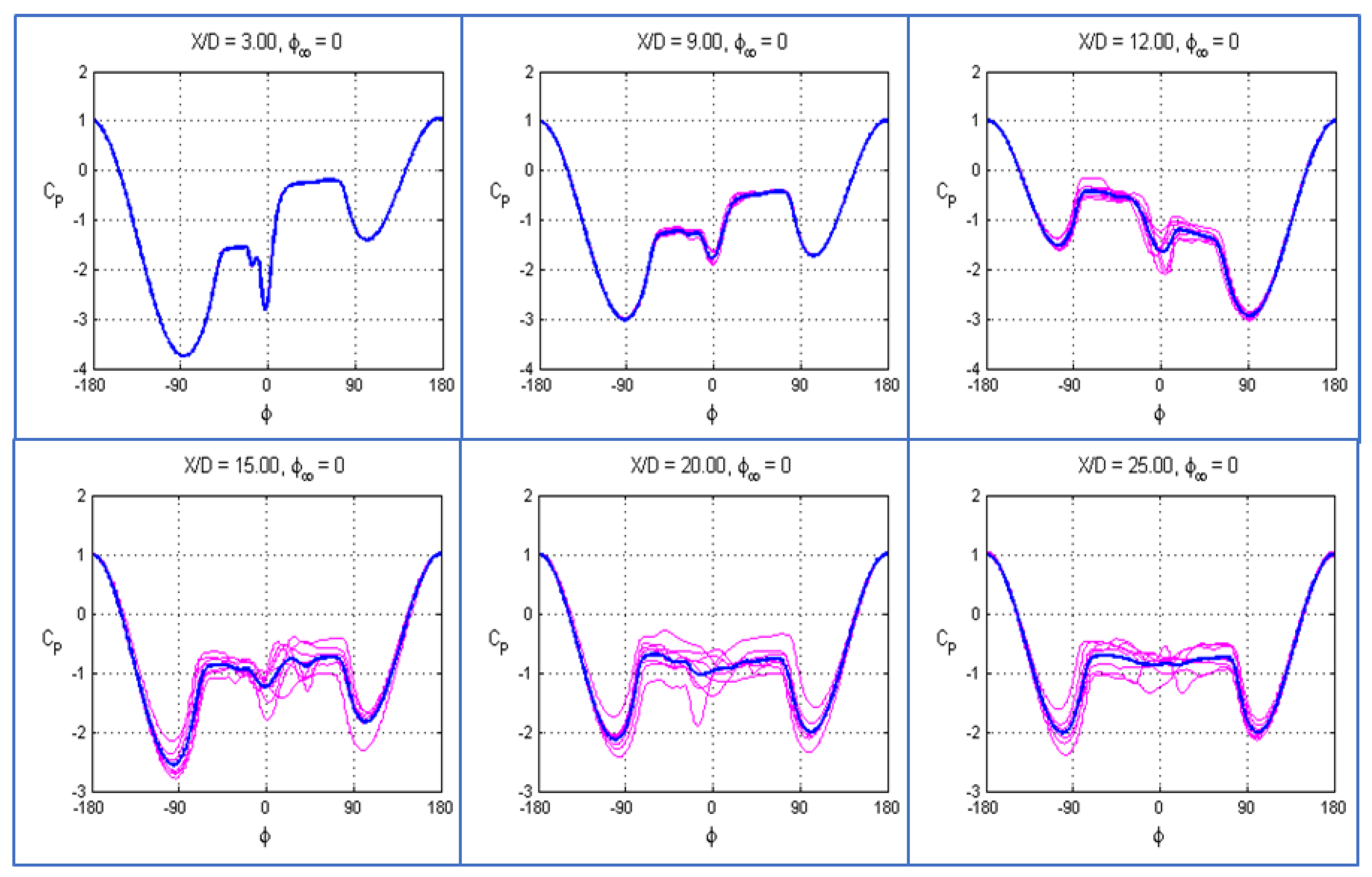
Figure 20 shows 20 instantaneous pressure coefficients in circumferential direction during a period of 0.1 s and their average at several x/D cross sections. The first two sections (x/D = 3.00 and x/D = 9.00) belong to Region 3 (the steady flow region), the next two sections (x/D = 12.0 and 15.00) belong to the unsteady Region 2 (with oblique vortices), and the last two sections (x/D = 20.0 and 25.00) belong to the unsteady flow Region 1, in which the alternating vortex Karman street pattern is appreciated. The legend is referred to the roll angle due to calculations at different roll angles being conducted. In this case, it is not relevant.

Figure 20.
Instantaneous and average pressure coefficient in a circumferential direction at several cross sections (long configuration).
Pressures at x/D = 3 and x/D = 9 present the characteristic steady asymmetric behavior of Region 3. Note that these stations are close to the second and fourth peaks of the sectional side force depicted in Figure 16a. Due to the spatial, though steady, alternation of vortices, the stronger depression occurs for negative values of Φ (port side). The pressures would be mirrored at stations near the third peak (x/D = 6.7). Pressures in Region 2 (x/D = 12 and x/D = 15) maintain the asymmetric behavior though introducing a level of unsteadiness. Note that the first station is close to a side-force peak (x/D = 12.1), whereas the last one is located between the peaks at x/D = 14.6 and x/D = 17, resulting in a lower level of asymmetry. Pressures at x/D = 20 and x/D = 25 exhibits a plateau in the leeside, whereas the instantaneous pressure coefficients display a change in the minimum value from one side to the other at a period of 0.1 s, indicating the von Karman street type of flow in this rear part of the body (Region 1).
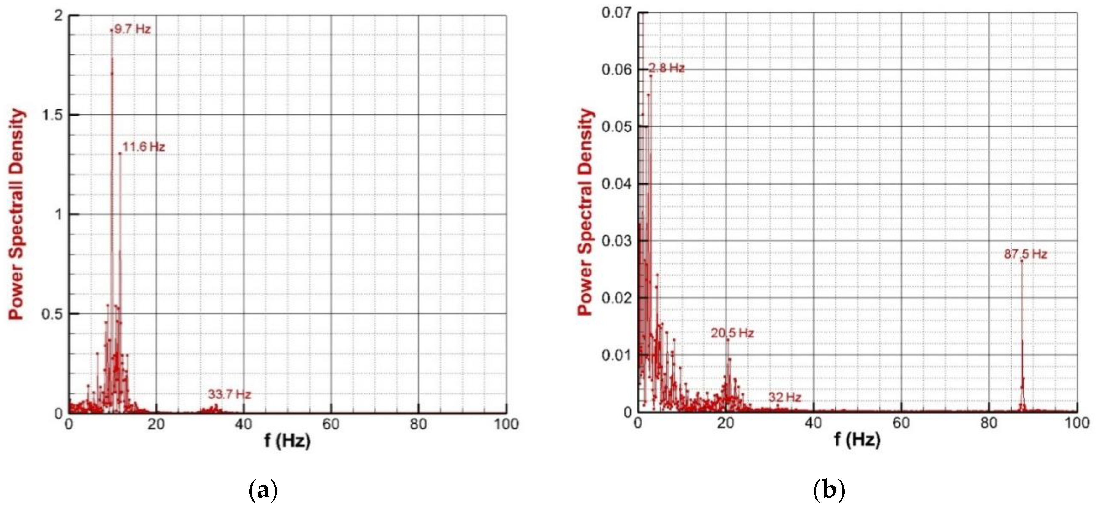
PSD provides an alternative means to visualize the effect of Karman street. Figure 21 shows the PSD of the side and normal force coefficients for the long configuration obtained over a period of 9 s.

Figure 21.
PSD of the side and normal force coefficients (long configuration). (a) Side force coefficient; (b) Normal force coefficient.
There are two low frequencies for the side force with significant peaks, 9.7 Hz and 11.6 Hz (St = 0.194 and St = 0.23), the first of which is very close to the value of 10 Hz obtained with a Strouhal number St = 0.2. The normal force, as in the reference case, presents amplitudes an order of magnitude lower. The corresponding figure displays some content of energy at low frequencies (2.8 Hz), a peak at 20.5 Hz, which relates to the Karman shedding (the normal force is independent of whether the vortex asymmetry is left or right-handed), and a high-frequency peak at 87.5 Hz.
It is important to remark again that for the correct prediction of the low-frequency part of the spectra of the forces it is needed a long physical time integration [22]. For this reference configuration, the time integration was t = 9.4 s (18800 Δt). This is a larger (more than double) period than that used for the calculation of the reference configuration (t = 4 s). However, the level of unsteadiness is larger. Therefore, the peaks at low frequencies observed in both the power spectral densities of the normal force coefficients of both configurations may be distorted by numerical noise. These low frequencies have little energy content for the side force coefficient of the long configuration (Figure 21a), while there is some content for the reference configuration (Figure 12a).
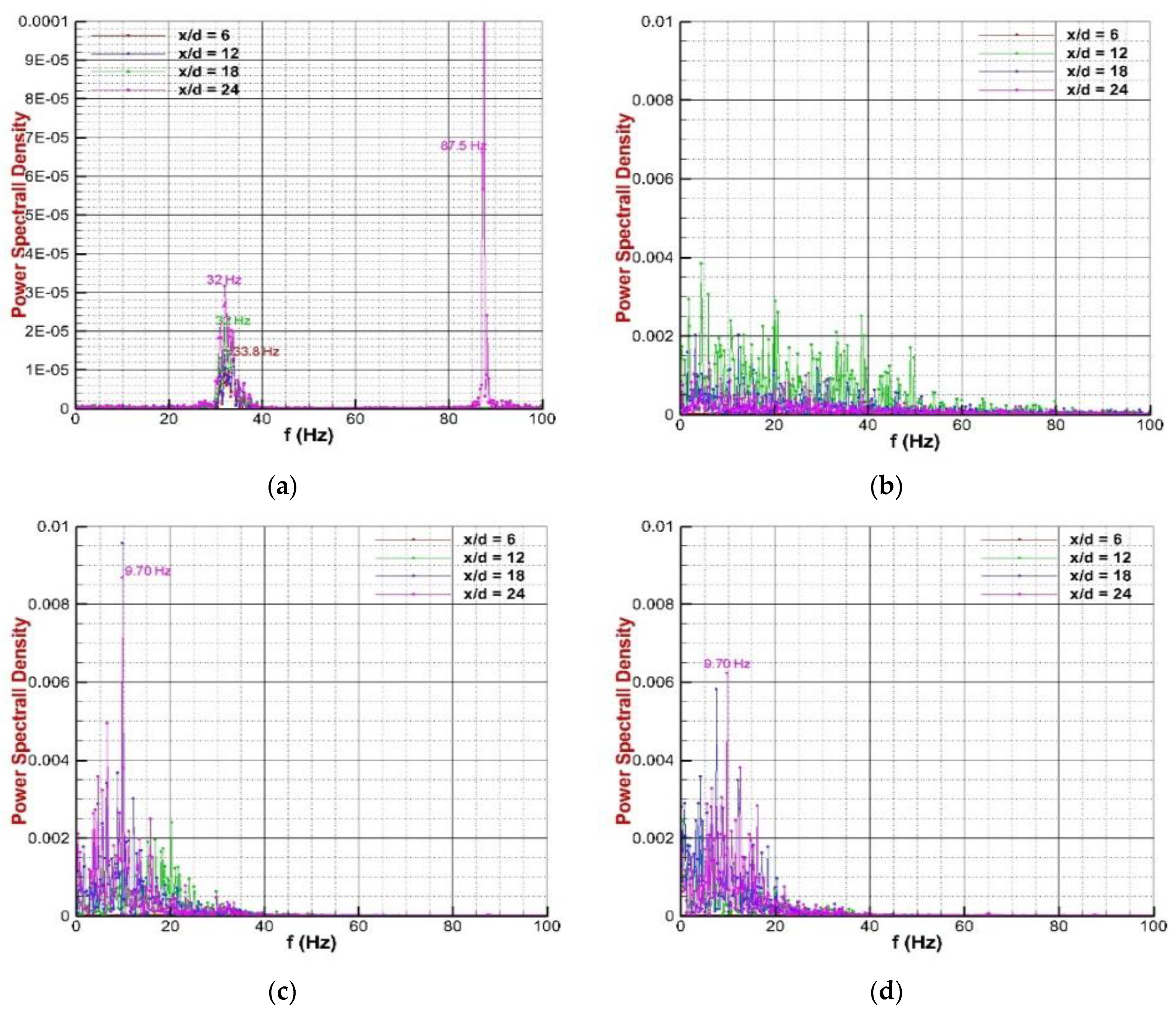
In order to obtain additional information, time histories for the pressure at four roll angles (Φ = 0, 180, 90, −90 deg.) and four cross sections (x/D = 6, 12, 18, 24) are shown in Figure 22. The roll angle Φ = 0 corresponds to the windward side. It is interesting to notice that the high-frequency peak of the normal force at 87 Hz may be due to an oscillation of the stagnation point at the rear part of the body (Region 1). This oscillation appears in the last second of the evaluated period. An oscillation at 33 Hz appears in the stagnation point at all sections, affecting both the side and normal force coefficients. The oscillations of separation lines correspond to the pressure oscillations shown in Figure 22 at the locations and occur in the Karman street region. They exhibit the dominant frequency of 9.7 Hz in Region 1.

Figure 22.
PSD of the pressure at four cross sections and four roll angles (long configuration). (a) Φ = 0 deg. (windward side); (b) Φ = 180 deg. (leeside); (c) Φ = 90 deg. (port side); (d) −90 deg. (starboard side).
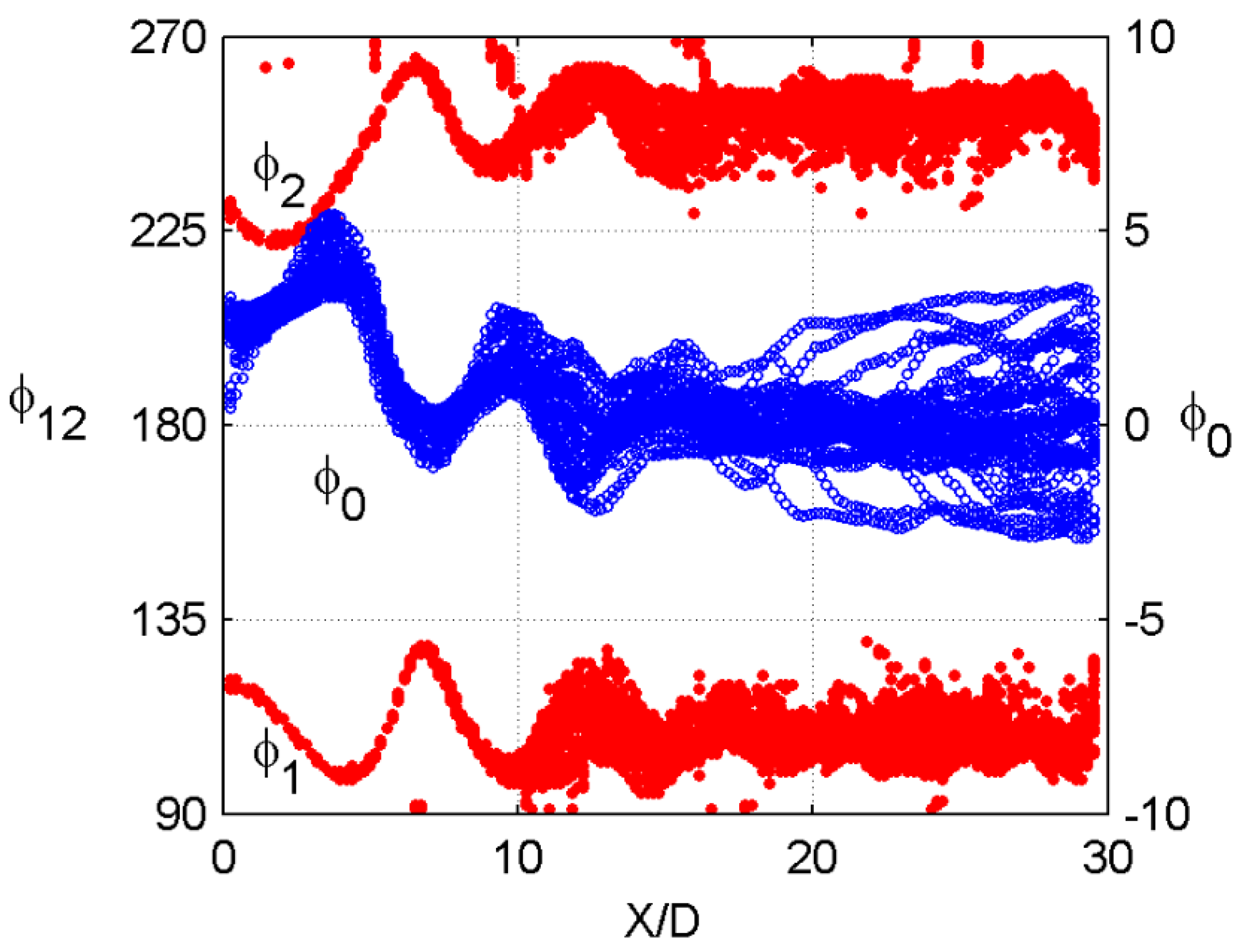
A plot of the separation lines (red color and left scale) together with the attachment line (blue color and right scale) is shown in Figure 23. There are some spurious values for the separation line plots due to the type of calculation of the minimum shear stress. The main conclusion obtained by looking at the figure is that the curves follow the same trend as the sectional side force coefficient curve (see Figure 16). However, there is apparently an important difference compared to the solution of the reference configuration (see Figure 15). The attachment line for the reference configuration was a thin line for sections x/D > 7.00, reinforcing the steady nature of the flow there, as shown by the sectional force coefficients, pressure coefficients and Q-contours curves (Figure 9, Figure 10 and Figure 13). In this case, the correspondent curves for the long configuration (Figure 16, Figure 17 and Figure 20) indicate that a steady flow Region 3 exists from the nose up to x/D = 10.0 approximately. The separation lines curves indicate this up to x/D = 10.0. Nevertheless, the attachment line does not show the same behavior. There is a small fluctuation of the attachment line in this region which does not significantly affect the resultant pressures and then the resultant sectional and global forces. The explanation for this apparent fluctuation of the stagnation line follows.

Figure 23.
Separation and attachment lines (long configuration).
First of all, the method of calculating this line is one seeking a minimum in a region that covers up to eight degrees (measured from ) where the values are very similar. The shear stress magnitude curve is flat. Small deviations can define a different position. It must be reminded that the cell size is 1.5 deg. and the attachment line can move from one cell to its neighbor cell. Then, a 1.5 deg. fluctuation observed in the nose region for the attachment line can be explained due to this method of calculation. Secondly, the pressure at the region close to indicates a small oscillation with a frequency of 32–33 Hz on the entire body (Figure 22), including the nose region. This is reflected in that the power spectral density of the side and normal force coefficients (Figure 21) show some energy content at this frequency. Then, a small fluctuation of the stagnation line may occur also in the named steady flow Region 3 which covers the fore body (up to x/D = 10 approximately).
The pressure oscillations at and regions indicated in Figure 22 occur at the rear body in Region 1 (From x/D = 20.0 to 30.0). The frequency corresponds to a St = 0.2, showing the Karman street-type region. The separation lines oscillate consequently, as shown in Figure 23.
We have indicated that it was detected an oscillation of the stagnation point at the rear part of the body (Region 1). This oscillation appears in the last second of the evaluated period, and it is a high-frequency oscillation (f = 87.5 Hz, see Figure 21 and Figure 22). At the rear part, there are two main frequencies for the stagnation line: 32 Hz and 87.5 Hz, while in Regions 2 and 3, only 32 Hz with lower amplitudes.
6. Conclusions
The flow past an axisymmetric ogive-cylinder configuration at a high angle of attack and low velocity has been numerically simulated using a URANS code. URANS with eddy viscosity turbulence models or Reynolds stress turbulence models fail to capture the unsteady flow regions. There is a need to use Scale-Adaptive Simulation (SAS) combined with Reynolds Stress turbulence models to compute the flow more accurately. SAS is an advanced URANS method with robust behavior with respect to space and time resolutions.
The effect of the fineness ratio was studied using a reference ogive-cylinder configuration with available experimental information. The numerical solutions calculated at a high angle of attack, where the flow is asymmetric, show that it becomes more unstable as the fineness ratio is increased. For a sufficiently long body, the distinct regions experimentally documented by several authors are clearly identified. The first region shows a von Karman vortex street-type flow, with alternating vortices and a zero averaged side force. It is located in the rear part of the body. The second region displays an asymmetric unsteady flow due to fluctuations in the strength and location of the eddies and the presence of many different turbulent structures. Finally, the region closer to the nose develops a steady asymmetric flow. For low and moderate fineness ratios, only Regions 2 and 3 are present.
Power Spectral Density analyses of the pressures and forces along different cross-sections allow us to separate the contributions of the different regions to the frequency content of the flow unsteadiness. Region 1 for the long body appears to be responsible for a peak very close to the value of 10 Hz obtained with St = 0.2, the characteristic Strouhal number of the Karman street of the cylinder in crossflow.
The good agreement between the sectional forces and pressure coefficients with their corresponding experimental data for the reference configuration allows an analysis of the flow structure with fair confidence.
Author Contributions
Conceptualization, J.J.-V.; Methodology, J.J.-V. and G.L.; Validation, G.L.; Investigation, J.J.-V.; Writing—original draft, J.J.-V. and G.L. All authors have read and agreed to the published version of the manuscript.
Funding
This research received no external funding.
Acknowledgments
The authors express their gratefulness to José Manuel Olalla Sánchez, from the Theoretical and Computational Aerodynamics Laboratory of the Flight Physics Department of INTA, who helped in the grid generation procedures.
Conflicts of Interest
The authors declare no conflict of interest. The funders had no role in the design of the study; in the collection, analyses, or interpretation of data; in the writing of the manuscript; or in the decision to publish the results.
References
- Menter, F.R.; Egorov, Y. A Scale Adaptive Simulation Model using Two-Equation Model. In Proceedings of the 43rd AIAA Aerospace Sciences Meeting and Exhibit, Reno, NV, USA, 10–13 January 2005. [Google Scholar] [CrossRef]
- Menter, F.R.; Egorov, Y. The Scale-Adaptive Simulation Method for Unsteady Turbulent Flow predictions. Part I: Theory and Model Description. Flow Turbul. Combust. 2010, 85, 113–138. [Google Scholar] [CrossRef]
- Menter, F.R.; Schütze, J.; Kurbatskii, K.A.; Gritskevich, M.; Garbaruk, A. Scale-Resolving Simulation Techniques in Industrial CFD. In Proceedings of the 6th AIAA Theoretical Fluid Mechanics Conference, Honolulu, HI, USA, 27–30 June 2011. [Google Scholar] [CrossRef]
- Menter, F.R.; Kuntz, M.; Bender, R. A Scale Adaptive Simulation Model for turbulent Flow Predictions. In Proceedings of the 41st Aerospace Sciences Meeting and Exhibit, Reno, NV, USA, 6–9 January 2003. [Google Scholar] [CrossRef]
- ANSYS FLUENT Theory Guide Release 19.1, ANSYS Inc. Southpointe 2600 ANSYS Drive, Canonsburg, PA 15317. 2018 April, pp. 92–95. Available online: https://t1.daumcdn.net/cfile/tistory/994B31465C0F6D991F?original (accessed on 23 March 2023).
- Champigny, P. High Angle of attack Aerodynamics. In AGARD Special Course on Missile Aerodynamics; Springer: New York, NY, USA, 1994; pp. 5-1–5-19. [Google Scholar]
- Champigny, P. Reynolds number effect on the aerodynamic characteristics of an ogive-cylinder at high angles of attack. In Proceedings of the 2nd Applied Aerodynamics Conference, Seattle, WA, USA, 21–23 August 1984. [Google Scholar] [CrossRef]
- Bridges, D.H. The Asymmetry Vortex Wake Problem- Asking the right Question. In Proceedings of the 36th AIAA Fluid Dynamics Conference and Exhibit, San Francisco, CA, USA, 5–8 June 2006. [Google Scholar] [CrossRef]
- Hunt, B.L. Asymmetric vortex forces and wakes on slender bodies. In Proceedings of the 9th Atmospheric Flight Mechanics Conference, San Diego, CA, USA, 9–11 August 1982. [Google Scholar] [CrossRef]
- Mahadevan, S.; Rodríguez, J.; Kumar, R. Effect of Controlled Imperfections on the Vortex Asymmetry of a Conical Body at high Incidence. In Proceedings of the 35th AIAA Applied Aerodynamics Conference, Denver, CO, USA, 5–9 June 2017. [Google Scholar] [CrossRef]
- Kumar, R.; Kumar, T.; Kumar, R. Role of Secondary shear-layer Vortices in the Development of Flow Asymmetry on a Cone-cylinder Body at high angles of incidence. Exp. Fluids 2020, 61, 215. [Google Scholar] [CrossRef]
- Ma, B.-F.; Huang, Y.; Deng, X.-Y. Dynamic Responses of asymmetric Vortices over slender Bodies to a rotating tip perturbation. Exp. Fluids 2016, 57, 54. [Google Scholar] [CrossRef]
- Jiménez-Varona, J.; Liaño, G.; Castillo, J.L.; García-Ybarra, P.L. Steady and Unsteady Asymmetric Flow regions past an axisymmetric Body. AIAA J. 2021, 59, 3375–3386. [Google Scholar] [CrossRef]
- Prananta, B.B.; Deck, S.; d’Éspiney, P.; Jirasek, A.; Kovak, A.; Leplat, M.; Nottin, C.; Petterson, K.; Wrisdale, I. Numerical Simulation of Turbulent and Transonic Flows about Missile Configurations, Final Report GARTEUR (AD) AG42 Missile Aerodynamics, Group for Aeronautical Research and Technology in Europe (GARTEUR), 20007, Tech. Report. NLR-TR-2007-704. Available online: https://researchgate.net/publication/224989541_Numerical_simulations_of_turbulent_subsonic_and_transonic_flows_about_missile_configurationsFinal_report_of_the_GARTEUR_AD_AG42_Missile_Aerodynamics (accessed on 23 March 2023).
- Ramberg, S.E. The effects of Yaw and Finite Length upon the Vortex Wakes of Stationary and Vibrating Circular cylinders. J. Fluid Mech. 1983, 128, 81–107. [Google Scholar] [CrossRef]
- Degani, D.; Tobak, M. Numerical Experimental and theoretical Study of convective Instability of Flows over Pointed Bodies at incidence. In Proceedings of the 29th Aerospace Sciences Meeting, Reno, NV, USA, 7–10 January 1991. [Google Scholar] [CrossRef]
- Zilliac, G.; Degani, D.; Tobak, M. Asymmetrci Vortices on a slender Body of Revolution. AIAA J. 1991, 29, 667–675. [Google Scholar] [CrossRef]
- Deane, J.R. An Experimental and Theoretical Investigation into the Asymmetry Vortex Flows Characteristics of Bodies of Revolution at High Angles of Incidence in Low Speed Flow, GARTEUR TP-109, Final Report of Group for Aeronautical Research and Technology in Europe (GARTEUR), GARTEUR AG04. 1984. Available online: https://garteur.org/ (accessed on 23 March 2023).
- Jiménez-Varona, J.; Liaño, G.; Castillo, J.L.; García-Ybarra, P.L. Roughness Effect on the Flow past Axisymmetric Bodies at high incidence. Aerospace 2022, 9, 668. [Google Scholar] [CrossRef]
- Degani, D. Development of nonstationary side forces along a slender body of revolution at incidence. Phys. Rev. Fluids 2022, 7, 124101. [Google Scholar] [CrossRef]
- Dubief, Y.; Delcayre, F. On coherent-vortex Identification in Turbulence. J. Turbul. 2011, 1, N11. [Google Scholar] [CrossRef]
- Egorov, Y.; Menter, F.R.; Lechner, R.; Cokljat, D. The Scale-Adaptive Simulation Method for Unsteady Turbulent Flow predictions. Part II: Application to Complex Flows. Flow Turbul. Combust. 2010, 85, 139–165. [Google Scholar] [CrossRef]
- Liaño, G.; Jiménez-Varona, J. Side Force on Bodies of revolution: Role of attached Flow. AIAA J. 2021, 59, 4475–4485. [Google Scholar] [CrossRef]


Disclaimer/Publisher’s Note: The statements, opinions and data contained in all publications are solely those of the individual author(s) and contributor(s) and not of MDPI and/or the editor(s). MDPI and/or the editor(s) disclaim responsibility for any injury to people or property resulting from any ideas, methods, instructions or products referred to in the content. |
© 2023 by the authors. Licensee MDPI, Basel, Switzerland. This article is an open access article distributed under the terms and conditions of the Creative Commons Attribution (CC BY) license (https://creativecommons.org/licenses/by/4.0/).