Experimental Aeroelastic Investigation of an All-Movable Horizontal Tail Model with Bending and Torsion Free-Plays

Abstract

In this study, an experimental investigation is performed on a scaled, all-movable horizontal tail to study the aeroelastic behaviors induced by multiple free-plays. The dynamic response in wind tunnel tests is measured by strain gauges, an accelerometer, and a binocular vision measurement system. The obtained results indicate that the present aeroelastic system exhibits highly nonlinear characteristics and undergoes two independent limit cycle oscillations (LCOs) induced by bending free-play and torsion free-play, respectively. Further, various parametric studies are conducted to evaluate the effects of the free-play angles, angle of attack, flow velocity, and gust excitation on the LCOs. It is found that the value of free-play angle has no significant effect on the critical flow velocity which leads to the occurrence of LCOs. The amplitude and frequency of LCOs increase with the increasing free-play angle and flow velocity. Moreover, the horizontal tail experiences high-order harmonic resonances when LCOs appear. Finally, the stability of limit cycles is analyzed based on the gust excitation experiment. Overall, compared to an all-movable horizontal tail with single free-play, the multiple free-plays system exhibits more complex dynamic behaviors. In this paper, the measured results of the scaled model, which has a similar mass distribution and stiffness distribution as actual aircraft, may be valuable for predicting such LCOs induced by multiple free-plays, and providing a reference for the design of all-movable horizontal tail to prevent LCOs.

1. Introduction

Nonlinear aeroelastic vibration is one of the major issues in aircraft design. Nonlinear vibration, characterized by limit cycle oscillation (LCO), can deteriorate the pilot handling quality, weapon-aiming capability, and fatigue life. Various mechanisms are recognized to induce LCO, such as structural, aerodynamic, and geometric nonlinearities [1,2,3,4,5]. These nonlinearities and their aeroelastic effect were well reviewed by Breitbach [6] and Lee et al. [7]. Among them, the structural nonlinearity caused by free-play is one of the main mechanisms that ultimately results in such self-excited oscillations in dynamic systems [8,9,10]. Therefore, the characteristics of free-play-induced LCO, which has a significant negative effect on the aeroelastic system, have been investigated extensively over the past few decades [11,12,13,14]. Further, actuator and bearing are dominating sources of free-play nonlinearity. Thus, assessing the impact of free-play on an all-movable horizontal tail, which has a complex actuating system, is of great importance for aircraft design.

Great efforts have been devoted to the study on nonlinear aeroelastic responses of all-movable horizontal tails with free-play [15,16]. Wu et al. [17] proposed a modeling method and an identification method, which were applied to an all-movable fin with free-play nonlinearity and verified by a ground vibration test. Hu et al. [18] analyzed the flutter and LCO responses of the horizontal tail by using an unstructured computational fluid dynamics solver coupled with finite element modal solver. Kim et al. [19] used the fictitious mass method to study the aeroelastic behavior of an all-movable wing with free-play. It is generally recognized that the initial conditions affect the LCO behavior significantly. Tang and Dowell [20] designed and constructed an all-movable horizontal tail model with flexible bending and torsion stiffness. Their results, measured in wind tunnel tests, indicated that the LCO amplitude increased with the flow velocity or free-play angle. Ni et al. [21] found that for an all-movable horizontal tail with free-play, the LCO would occur at a much lower flow velocity than that without free-play. Arévalo and García-Fogeda [22] presented a time domain approach to the flutter analysis of a missile-type wing/body configuration with free-play nonlinearity, and observed LCOs and chaotic motion below the flutter speed. Kim and Lee [23] analyzed the nonlinear aeroelastic response of a flexible airfoil with pitch free-play. LCOs and chaotic motion were observed, and they were highly influenced by the pitch-to-plunge frequency ratio. In addition, some studies showed that the free-play angle cannot be the only significant parameter involved in the free-play criteria (MIL-A-8870). Chen et al. [24] presented the LCO characteristics of a scaled horizontal tail model with free-play and angle of attack. They found that in addition to the free-play angle, the angle of attack is also an important parameter affecting the LCO. Chen and Lee [25] investigated the effect of the flight-loads on the LCO induced by free-play. Their results suggested that, due to ignoring the loading condition, the current military specification for free-play limit is probably too stringent. In fact, almost no operational airplane with an all-movable horizontal tail meets this requirement. Moreover, in a recent paper by Zhang et al. [26], it was demonstrated numerically that flap hinge free-play combined with cubic pitching stiffness may lead to LCO at a flow velocity well below the flutter speed of the linear system. In the absence of strong structural damping, the combined nonlinearity may induce complex dynamic responses. The study by Tian et al. [27] also showed that the all-movable fin with pitch and flap free-plays exhibited more complex dynamic responses than that with single free-play nonlinearity.

Overall, the previous research provides some significant insights into all-movable horizontal tail designs and free-play-induced LCO characteristics. However, most existing studies on structural nonlinearity have focused on the single free-play system, and little attention has been paid to the effect of multi-free-plays on the aeroelastic behaviors of the all-movable horizontal tail.

This study is based on a scaled all-movable horizontal tail model that features the following characteristics: multiple free-play angles are adjustable, and the beam-rib–skin structure is similar to that used in actual aircraft. The present paper sheds light on the effects of free-play angles, flow velocity, and gust excitation on LCO behavior. In Section 2, a design method of the all-movable horizontal tail model with bending and torsion free-plays is proposed. The details about the experimental setup and methodology are provided in Section 3. In Section 4, discussions are provided to clarify the aeroelastic characteristics of the single-free-play system and multi-free-plays system based on wind tunnel tests. Finally, the main findings and conclusions are summarized in Section 5.

2. Experimental Model

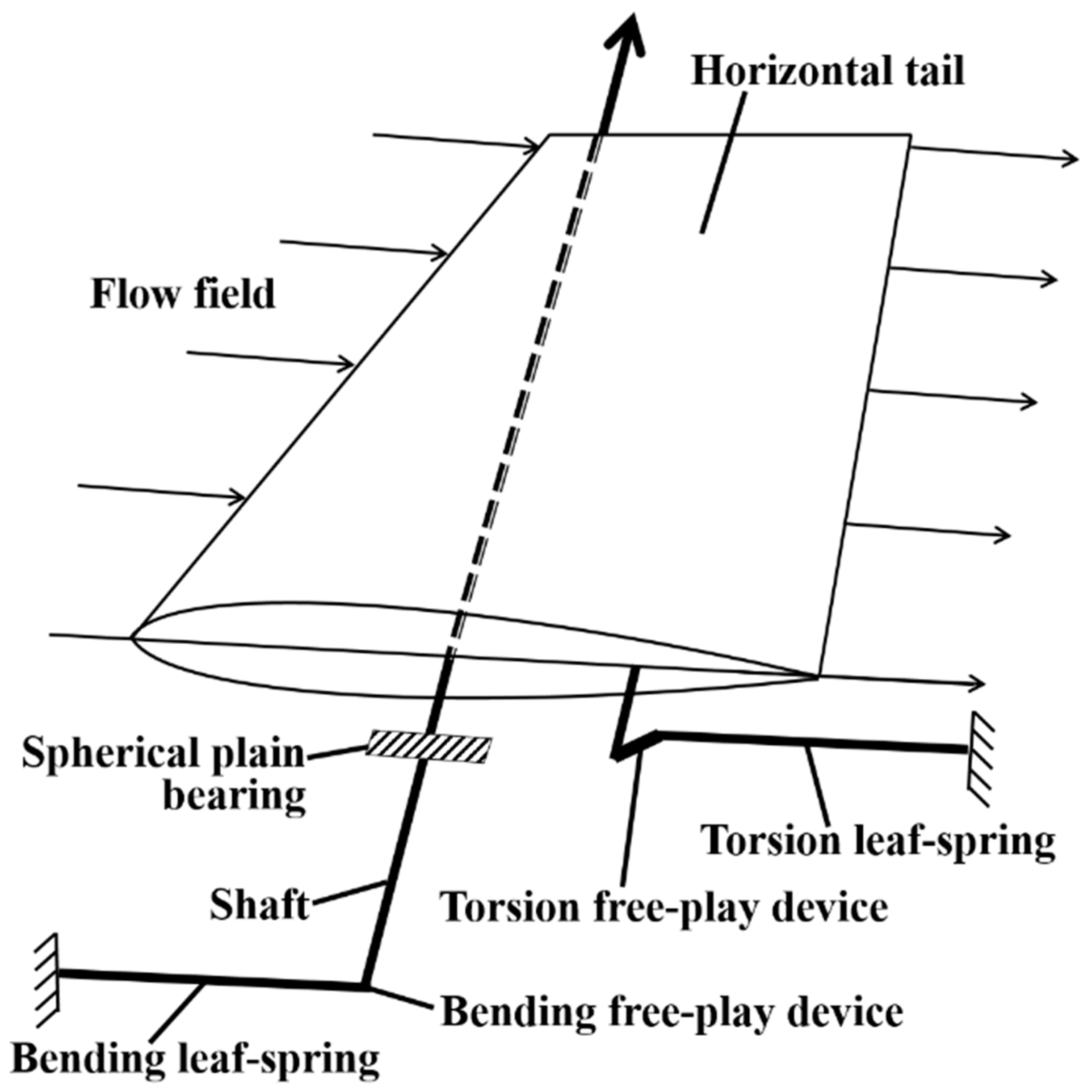
2.1. The Principle of the Model

An experimental model with bending and torsion free-plays was constructed to observe and measure the aeroelastic response of an all-movable horizontal tail with multi-free-plays. The schematic of this horizontal tail is shown in Figure 1. It can be seen that the horizontal tail was connected to the free ends of the bending leaf-spring and torsion leaf-spring. Based on this, the model could carry out bending and torsion vibrations centered on the spherical plain bearing. In addition, a bending free-play device and a torsion free-play device were used to simulate the free-plays in the actuating system.

Details of the bending free-play device are shown in Figure 2a. The bending free-play pin was connected to the shaft through thread to achieve a tight fit. Additionally, the middle section of bending free-play pin was sheathed in connector A, while the diameter of the middle section of bending free-play pin was smaller than the inner diameter of connector A to achieve a clearance fit. Similarly, the torsion free-play pin fit tightly with connector B; see Figure 2b. Simultaneously, connector C and the middle section of the torsion free-play pin were in clearance fit. The torsion free-play angle could be adjusted by changing the diameter of the middle section of the torsion free-play pin. In addition, the distance between the horizontal tail and the torsion leaf-spring was variable by adjusting the length of connector C, resulting in the horizontal tail rotation to simulate the initial angle of attack.

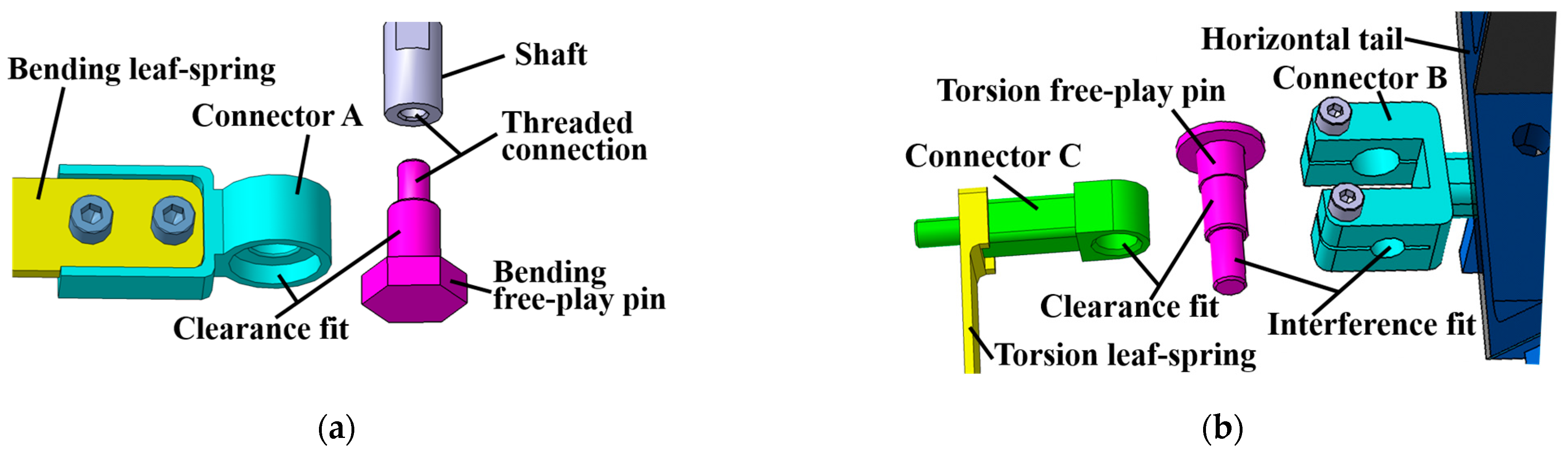
2.2. Model Design and Manufacture

Subsequent wind tunnel tests were performed in a low-speed closed-circuit wind tunnel at Shenyang Aerospace University. The height, width, and length of the wind tunnel experimental section were 1 m, 1.2 m and 3 m, respectively. The turbulence level of the wind tunnel was less than 0.14%. According to the parameters of the low-speed wind tunnel, the geometric features of the wind tunnel model were selected, as shown in

Table 1. Geometric features of the horizontal tail model.

Description	Value
The length of root chord, mm	659.1
The length of tip chord, mm	220.3
The length of span, mm	650.6
Swept angle of the leading edge, deg.	34
Airfoil	NACA 0012
The thickness of skin, mm	1.0
The thickness of ribs, mm	1.0
The thickness of beams (from leading edge to trailing edge), mm	3.5, 6.0, and 2.0
The length and diameter of the shaft, mm	111.0 and 8.0
The length, height, and thickness of the bending leaf-spring, mm	141.0, 20.0, and 3.5
The length, height, and thickness of the torsion leaf-spring, mm	237.0, 16.0, and 3.2

. In addition, the lengths of the root chord, tip chord, and span were referenced to a jet aircraft and scaled down by one third. The wind tunnel model adopted the beam-rib–skin structure commonly used in actual aircraft. Beam-ribs with variable cross-section were applied to the horizontal tail model to obtain a reasonable mass distribution and stiffness distribution. Compared to the flat-plate wing model, the present three-dimensional model may have more similar dynamic characteristics to the actual aircraft [28,29,30,31,32]. In addition, the thicknesses of the bending and torsion leaf-springs were selected as 3.5 mm and 3.2 mm, respectively. The stiffnesses of the bending and torsion leaf-springs were 15,754 N/m and 2028 N/m, respectively.

The computer-aided design model displayed the structural details of the horizontal tail more clearly, as shown in Figure 3a. A streamlined fairing with a length of 1826 mm was used to form a stable flow field in the wind tunnel test. In addition, the functions of load point and accelerometer will be illustrated in Section 3. The components of the model were made of the materials listed in

Table 2. Materials of the components.

Components	Materials
Beam-rib–skin structure	GFRP (Glass fiber reinforced plastics)
Fairing	Pine and GFRP
The joint of the tail root and the shaft	Aluminum alloy
Leaf-springs and shaft	Steel

. The manufactured horizontal tail model weighed 2.2 kg, as shown in Figure 3b.

3. Experimental Setup and Methodology

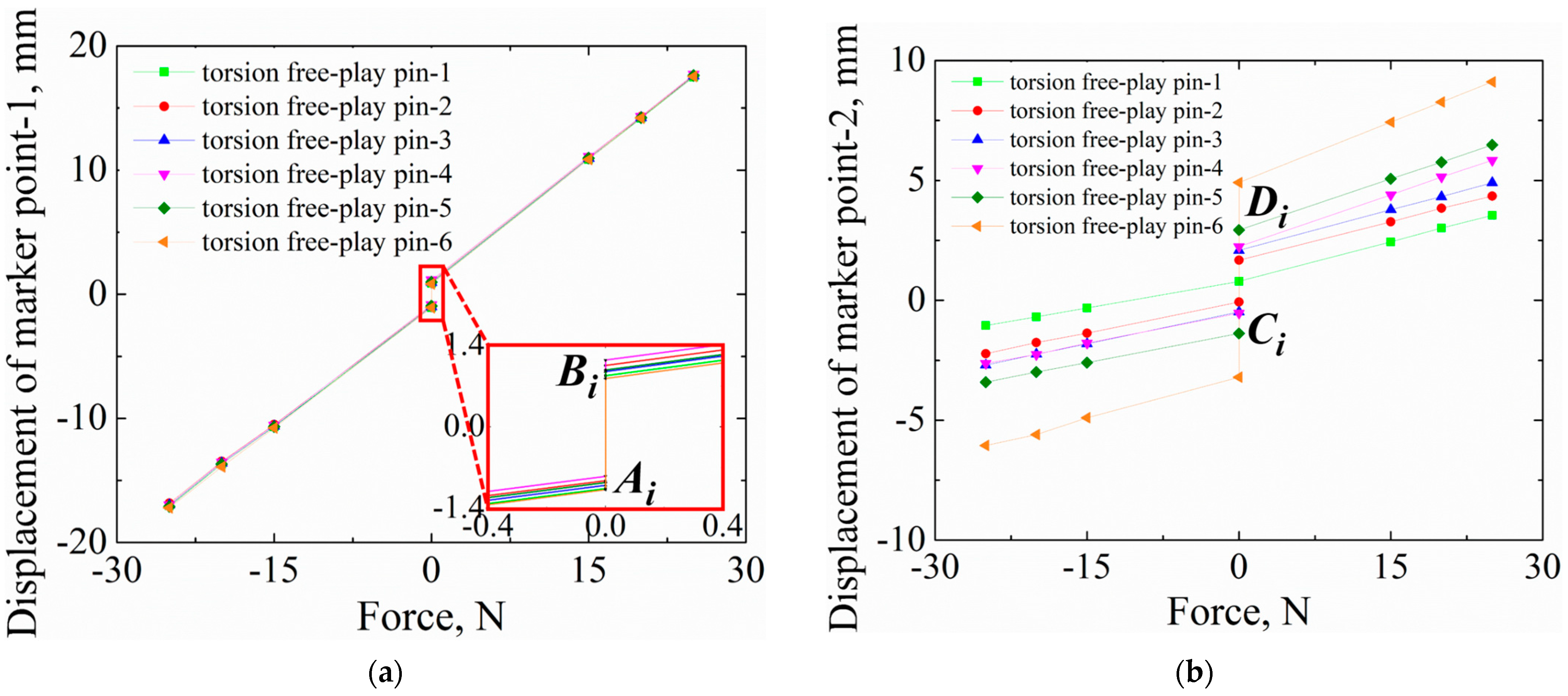
3.1. Free-Plays and Angle of Attack Measurements

In this section, free-plays and angle of attack were measured. As shown in Figure 4, a loading point was placed at 497.9 mm from the root and 168.8 mm from the trailing edge. The marker point-1 was placed at the intersection of the leading edge and the extension line of the shaft, and the marker point-2 was placed at the root of the trailing edge. In this paper, six torsion free-play pins with different middle section diameters and one bending free-play pin were designed and machined. For each torsion free-play pin, a set of pulling forces were exerted on both sides of the loading point. Displacements of two marker points under these pulling forces were measured using a binocular vision measurement system.

Six sets of measurements for marker point-1 are shown in Figure 5a. For the ith torsion free-play pin, intersections of the measured pulling force-displacement curve and Y-axis were calculated using the least square method, indicated by A_i and B_i. The interval between A_i and B_i represents the free range-of-motion of the horizontal tail induced by bending free-play when the pulling force is 0. Here, Y_Ai and Y_Bi represent the Y-axis coordinate values of A_i and B_i (Y_Bi > Y_Ai). According to the geometric features of the model, the bending free-play angle δ_b can be calculated by using Equation (1).

$${\delta }_b=360 \left(\overline{Y_{Bi}} – \overline{Y_{Ai}}\right)/4\pi H \left(i=1, 2, 3, 4, 5, 6\right)$$

(1)

where H = 584.1 mm is the distance from the center of bearing to the marker point-1. Thus, the calculated bending free-play angle δ_b = ±0.10°.

The results of marker point-2 are shown in Figure 5b. Similarly, C_i and D_i represent the intersections of the force-displacement curve and the Y-axis for the ith torsion free-play pin, and Y_Ci and Y_Di are used as the values of Y-axis coordinates of C_i and D_i (Y_Di > Y_Ci). The interval between Y_Di and Y_Ci represents the free range-of-motion of the horizontal tail caused by the ith torsion free-play when the pulling force is 0. Moreover, the center point of C_i and D_i corresponds to the initial angle of attack related to torsion DOF. Torsion free-play angles δ_t and angle of attack α can be obtained by using the following equations:

$${\delta }_{ti}=360\left(Y_{Di} – Y_{\mathrm{C}i}\right)/4\pi h \left(i=1, 2, 3, 4, 5, 6\right)$$

(2)

$$\alpha =360\left(\overline{Y_{\mathrm{C}i}}+\overline{Y_{Di}}\right)/4\pi h \left(i=1, 2, 3, 4, 5, 6\right)$$

(3)

where h = 302.9 mm is the distance from the center of bearing to the marker point-2. The calculated angle of attack α = 0.15°, and the torsion free-play angles are ±0°, ±0.165°, ±0.243°, ±0.262°, ±0.409°, and ±0.767°, respectively. Therefore, the experimental investigations of aeroelastic response induced by single free-play or multiple free-plays can be carried out by using different combinations of bending free-play pin and torsion free-play pins.

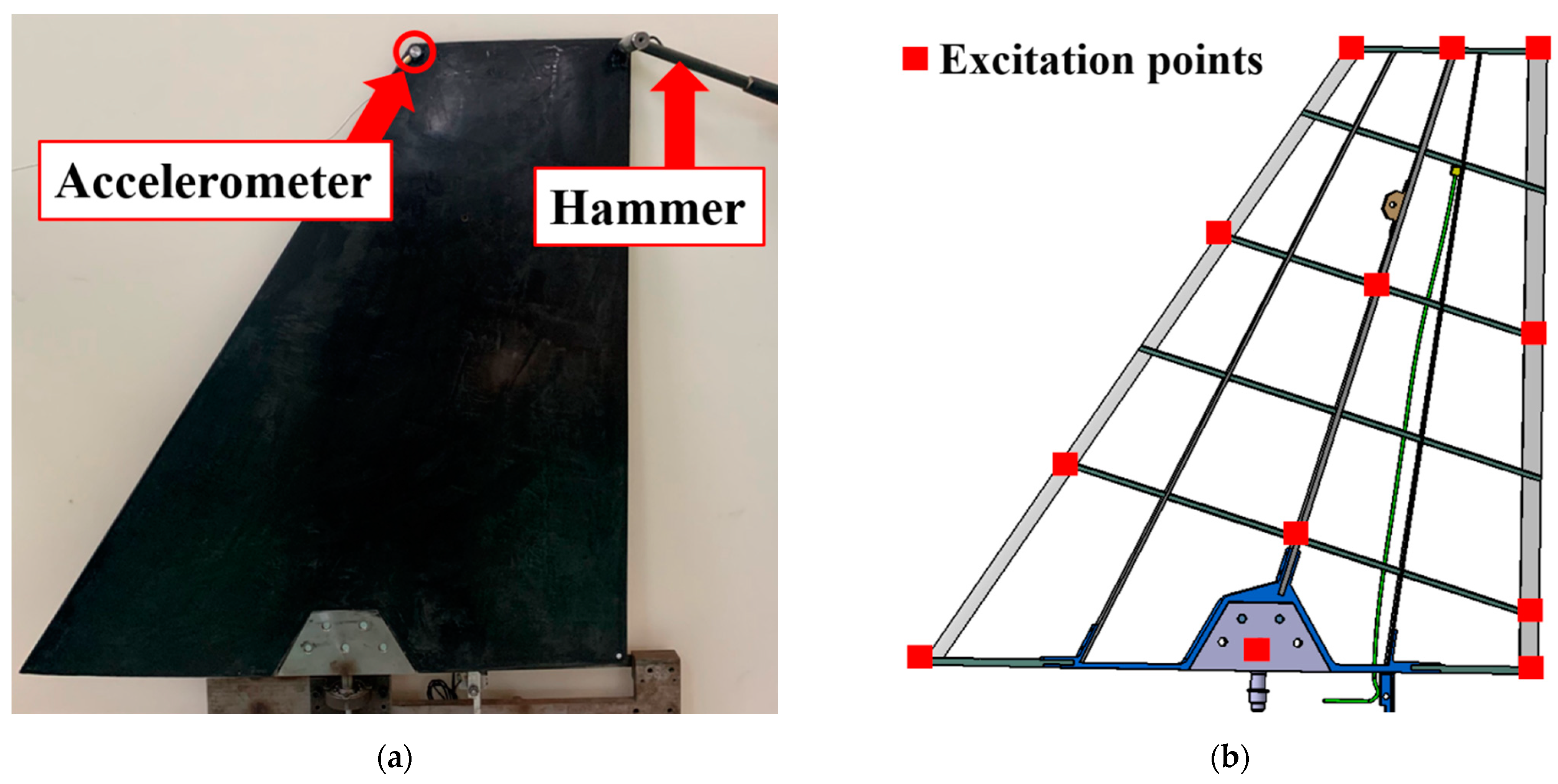
3.2. Ground Vibration Test

The ±0° torsion free-play pin was chosen for the ground vibration test (GVT) to analyze the basic dynamic characteristics of the horizontal tail model, as shown in Figure 6. The first bending frequency and the first torsion frequency measured in GVT were 4.5 Hz and 19.9 Hz, respectively. Corresponding damping coefficients were 1.18% and 1.24%, respectively. Modes obtained by GVT are shown in Figure 7.

A finite element model consistent with the experimental model was constructed. The first bending frequency and the first torsion frequency were 4.6 Hz and 20.1 Hz, respectively, which was in good agreement with the GVT results. Applying a force of 1 N at marker point-1, the calculated displacements of marker point-1 with and without leaf-springs were 1.7 mm and 0.4 mm, respectively. When the force was applied to marker point-2, the displacements of marker point-2 with and without leaf-springs were 2.0 mm and 0.4 mm. The calculated flutter speed of the linear system without free-plays was 77 m/s.

3.3. Data Acquisition in Wind Tunnel Tests

The experimental model installed in the wind tunnel is shown in Figure 8a. The aeroelastic response in the wind tunnel tests was measured in the following ways:

• Two strain gauges were glued to near the fixed end of the leaf-springs and were used to measure the bending angle and torsion angle. The experimental sampling rate was 128 points per second, and the sampling length was 3840 points;
• A built-in shear piezoelectric accelerometer manufactured by PCB piezotronics incorporated was placed inside the skin of the model (i.e., as shown in Figure 3a: the position of the accelerometer was 534.1 mm from the root and 96.4 mm from the trailing edge). The sensitivity of the accelerometer was 100.0 mV/g (10.20 mV/m/s²). The experimental sampling rate was set to 128 Hz;
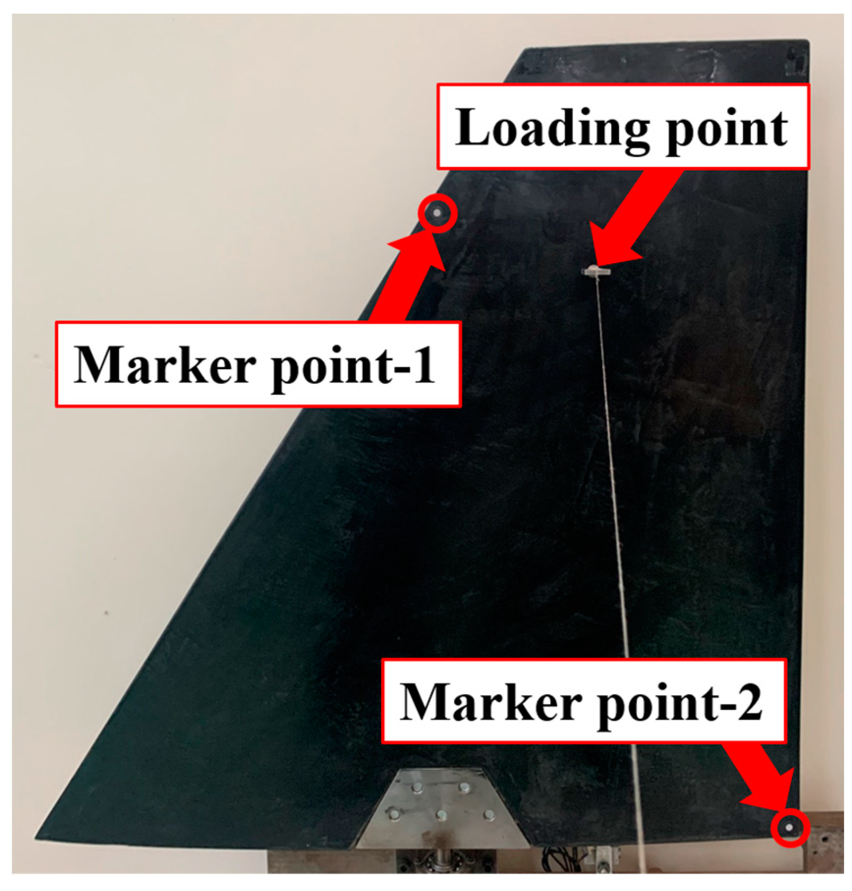
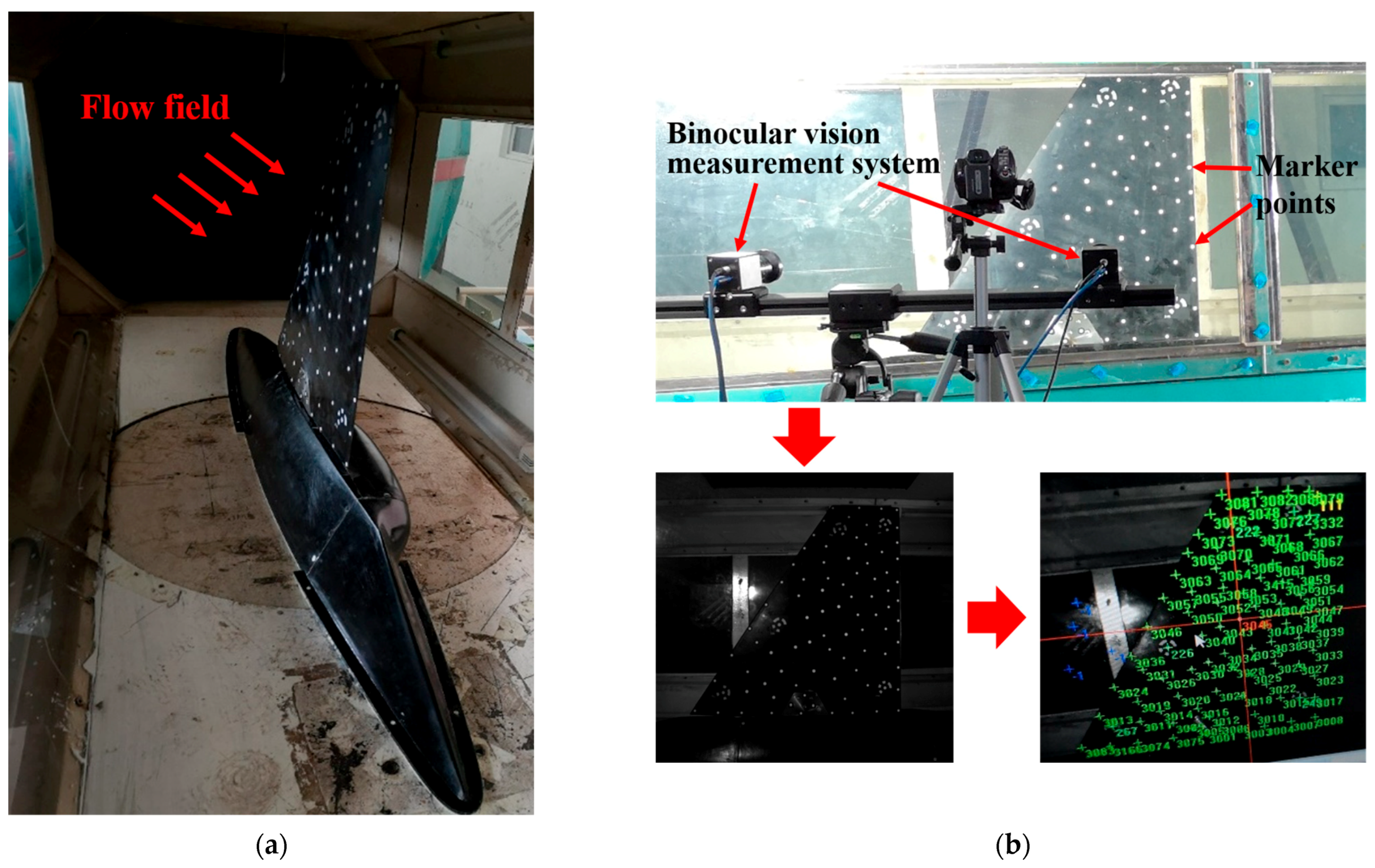
• A set of marker points was pasted on one side of the model to obtain the transient states during the vibration process (i.e., the instantaneous displacement of each marker point could be measured by the binocular vision measurement system with a sampling frequency of 43 Hz, as shown in Figure 8b).

Additionally, the data were collected after the flow velocity stabilized. The output signals from these transducers were directly recorded on a computer with data acquisition and analysis software.

4. Results and Discussions

4.1. Aeroelastic Response of the Single Free-Play System

All single free-play experiments were performed with ${\delta }_b=0.1°$, ${\delta }_t=0°$, and α = 0.15° to investigate the effect of bending free-play on the response of the model. The system underwent three stages of slight random vibration/LCO/slight random vibration with the flow velocity varying from 5 to 35 m/s. The time histories of the bending angle and torsion angle at V = 19 m/s, V = 20 m/s, V = 21 m/s, and V = 35 m/s are shown in Figure 9, which indicates that the LCO induced by bending free-play was observed at V = 20 m/s and then disappeared at V = 21 m/s. A similar characteristic related to torsion free-play was proposed by Tang and Dowell [16], and it was demonstrated that such a disappearance of the LCO could be attributed to the initial non-zero angle of attack. The model continued to experience slight random vibration when the flow velocity rose from 21 to 35 m/s. The maximum flow velocity of the test was selected as 35 m/s for the following reasons: (1) to avoid model damage; (2) to avoid the wind tunnel being damaged by the broken model; and (3) because the flow velocity was close to the wind tunnel boundary, and a further increase of the flow velocity may reduce the stability of the flow field. In the following section, this LCO, which appeared at V = 20 m/s, will be further investigated.

4.2. Aeroelastic Response of Multiple Free-Plays System

All the following experiments were performed with the initial conditions for bending free-play angle ${\delta }_b=0.1°$ and angle of attack α = 0.15°. In addition, five torsion free-play angles varying from${\delta }_t=0.165°$ to $0.767°$ were employed to study the LCO behaviors induced by multiple free-plays quantitatively. The same phenomenon found in the five groups of experiments was that the model experienced four processes of slight random vibration/small amplitude LCO/slight random vibration/large amplitude LCO as the flow velocity increased. For convenience, these two LCOs are referred to herein as S-LCO (small amplitude LCO) and L-LCO (large amplitude LCO), respectively. The time histories of bending angle and torsion angle at V = 19 m/s, V = 20 m/s, V = 21 m/s, and V = 27 m/s are shown in Figure 10a,b, respectively (${\delta }_t=0.767°$ is taken as an example). Displacement-velocity phase diagrams are shown in Figure 11. From Figure 10 and Figure 11, the following points can be drawn:

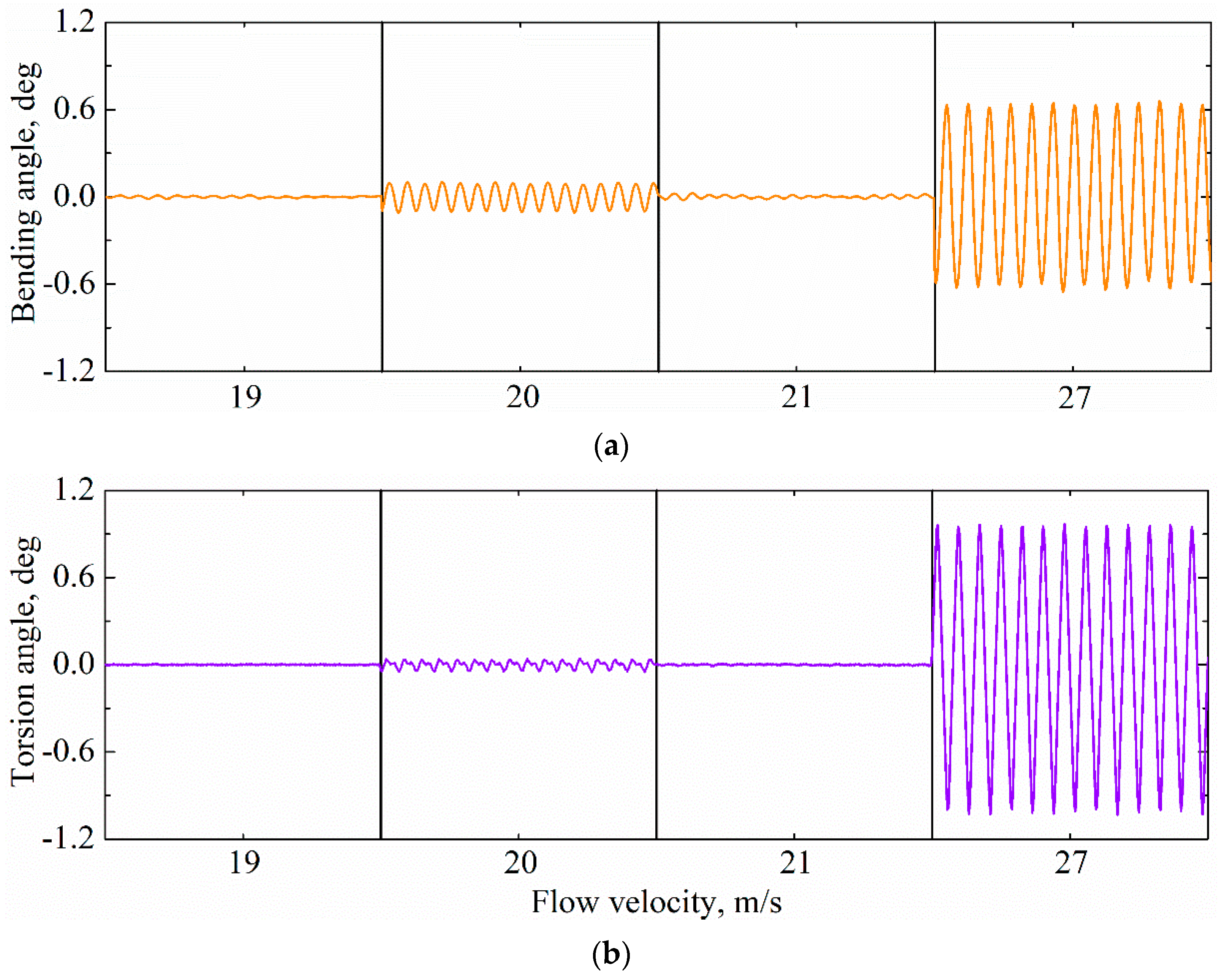
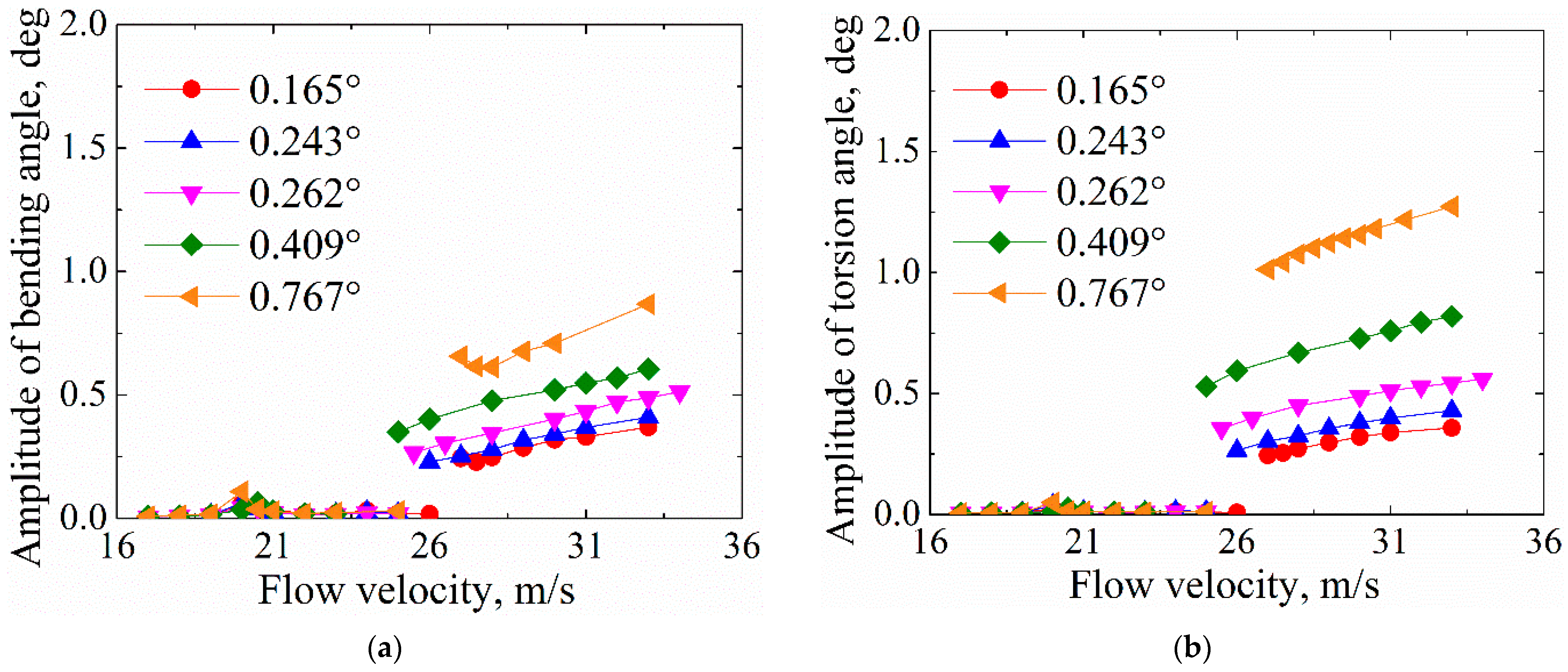
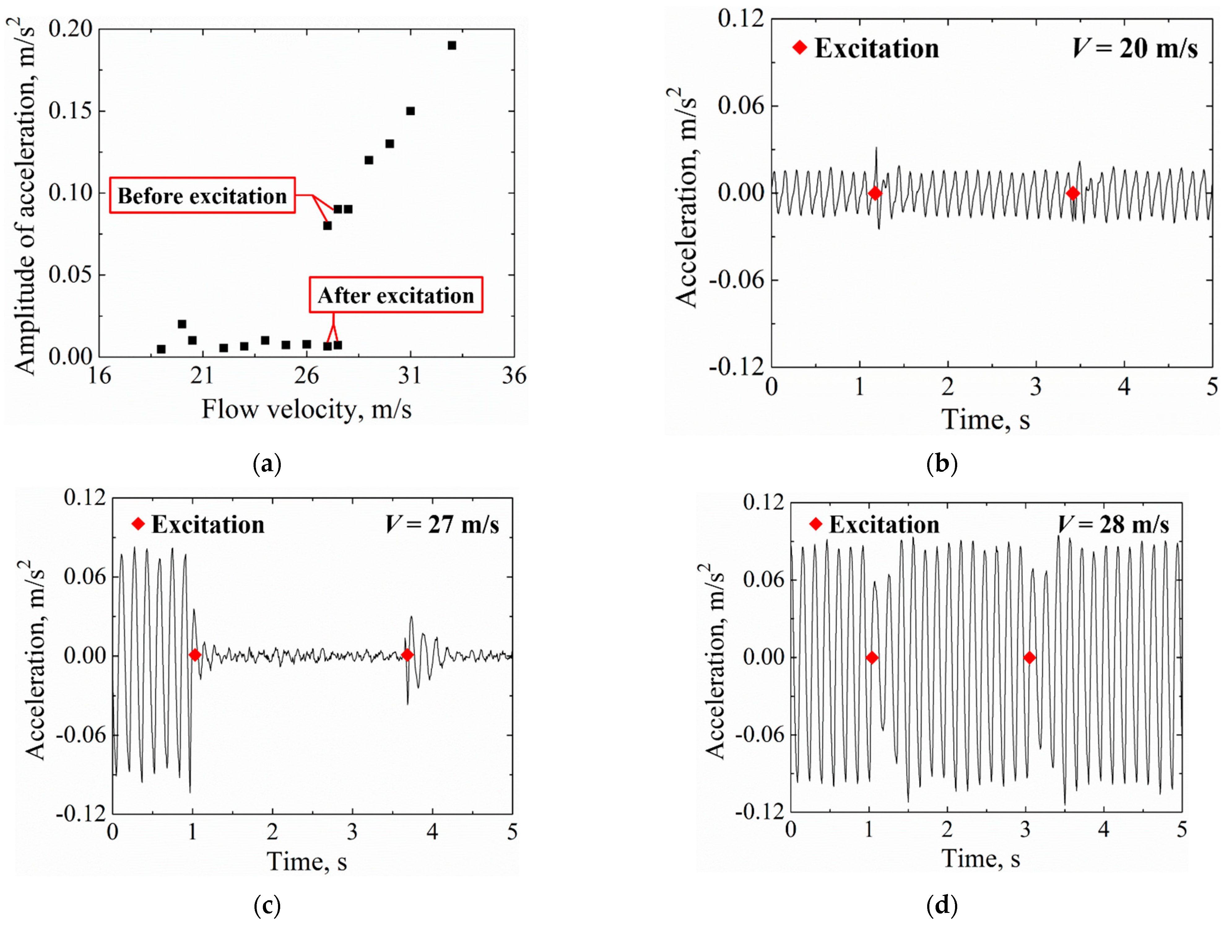
• The S-LCO appeared at V = 20 m/s and disappeared at V = 21 m/s, which is the same as the result in Section 4.1. Moreover, the L-LCO occurred when the flow velocity increased to 27 m/s. Therefore, it can be inferred that the L-LCO was caused by the torsion free-play. In addition, for simplicity, the critical flow velocities that led to the occurrences of S-LCO and L-LCO are called V_S-LCO and V_L-LCO, respectively;
• For S-LCO, the amplitude of bending angle was greater than that of torsion angle. However, the opposite was true for the L-LCO;
• For the L-LCO induced by torsion free-play, the vibration characteristics were very different in the free-play region and the stiffness region (see Figure 11b, V = 27 m/s). The torsion velocity was relatively stable in the free-play region, but it was more variable in the stiffness region.

According to the measured instantaneous displacement of each marker point, the transient states within one vibration period of the S-LCO and the L-LCO were obtained by the digital image correlation method [33,34,35], as shown in Figure 12a,b, respectively. The results show that the S-LCO mainly contained bending vibration, while the L-LCO contained both bending vibration and torsion vibration.

For different torsion free-play angles, the amplitudes of bending angle and torsion angle vs. flow velocity are shown in Figure 13a,b, respectively. The results show that the value of torsion free-play angle hardly affected the ${\mathrm{V}}_{\mathrm{S}-\mathrm{L}\mathrm{C}\mathrm{O}}$ and${\mathrm{V}}_{\mathrm{L}-\mathrm{L}\mathrm{C}\mathrm{O}}$. Furthermore, the value of torsion free-play angle had no significant effect on the amplitudes of bending angle and torsion angle in S-LCO. However, when $\mathrm{V}\ge {\mathrm{V}}_{\mathrm{L}-\mathrm{L}\mathrm{C}\mathrm{O}}$, the amplitudes of bending angle and torsion angle increased prominently with the increasing torsion free-play angle and flow velocity.

The quantitative analysis carried out using the same data in Figure 13 is shown in Figure 14, in which the amplitudes of bending angle and torsion angle are non-dimensionalized by the torsion free-play angle. These non-dimensional values indicate the effect of the torsion free-play angle on the LCO amplitude more clearly. The results show that the non-dimensional amplitudes of torsion angle were nearly the same for all torsion free-play angles (see Figure 14b). Thus, it can be determined that the amplitude of torsion angle was almost proportional to the torsion free-play angle, while such a rule does not apply to the amplitude of bending angle (see Figure 14a).

The ratio of torsion angle amplitude to bending angle amplitude vs. flow velocity for different torsion free-play angles was calculated to further explain the effect of torsion free-play angle on amplitude; see Figure 15. Interestingly, when $\mathrm{V}<{\mathrm{V}}_{\mathrm{L}-\mathrm{L}\mathrm{C}\mathrm{O}}$, ${\theta }_t/{\theta }_b$ was less than 1 and reached its minimum value at $\mathrm{V}={\mathrm{V}}_{\mathrm{S}-\mathrm{L}\mathrm{C}\mathrm{O}}$. When $\mathrm{V}\ge {\mathrm{V}}_{\mathrm{L}-\mathrm{L}\mathrm{C}\mathrm{O}}$, ${\theta }_t/{\theta }_b$ was greater than 1 and increased as the torsion free-play angle increased. This shows that a larger torsion free-play angle leads to more torsion vibration in L-LCO.

Fast Fourier transform (FFT) was performed on the measured acceleration to obtain the main frequency at different flow velocities, as shown in Figure 16. When $\mathrm{V}<{\mathrm{V}}_{\mathrm{L}-\mathrm{L}\mathrm{C}\mathrm{O}}$, the frequency increased almost linearly with the increase in flow velocity and was independent of torsion free-play angle. The frequency dropped at $\mathrm{V}={\mathrm{V}}_{\mathrm{L}-\mathrm{L}\mathrm{C}\mathrm{O}}$ and subsequently increased slightly with the flow velocity and torsion free-play angle.

In addition, high-order harmonics were observed in the FFT frequency spectra and the characteristics of the high-order harmonics were related to the torsion free-play angle. Therefore, two torsion free-play angles (${\delta }_t=0.767°$ and ${\delta }_t=0.243°$) were selected for further analysis. The fundamental frequency and high-order frequency at different flow velocities are shown in Figure 17a and Figure 18a. The FFT frequency spectra for two torsion free-play angles at V = 20 m/s, V = 27 m/s and V = 33 m/s are shown in Figure 17b–d and Figure 18b–d, respectively. It is interesting to note that high-order harmonics always appear along with LCOs. From Figure 17 and Figure 18, the following points can also be made:

• Second/third order harmonics always prominently exist in S-LCOs (see Figure 17b and Figure 18b) and L-LCOs (see Figure 17c,d and Figure 18c,d), respectively;
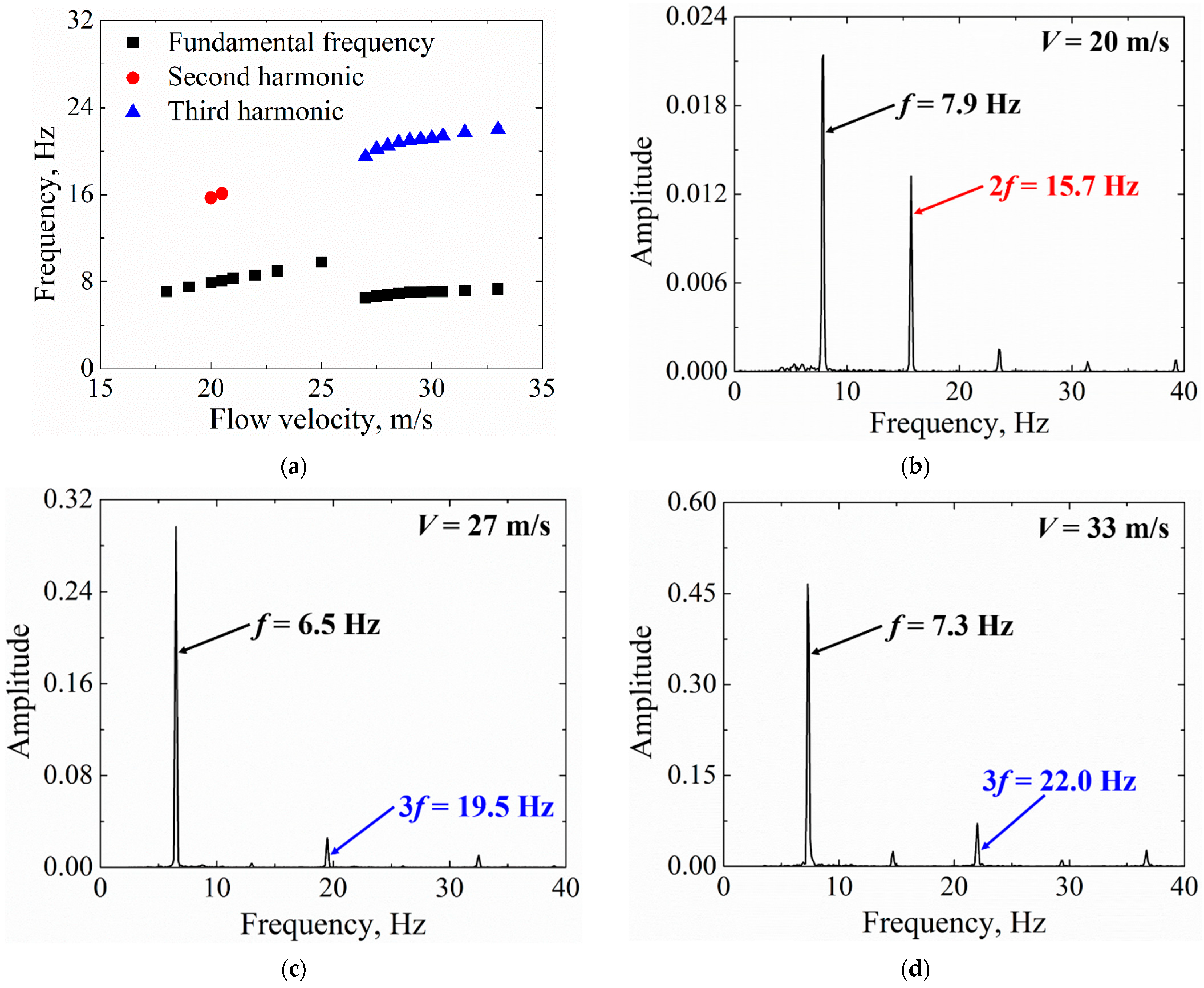
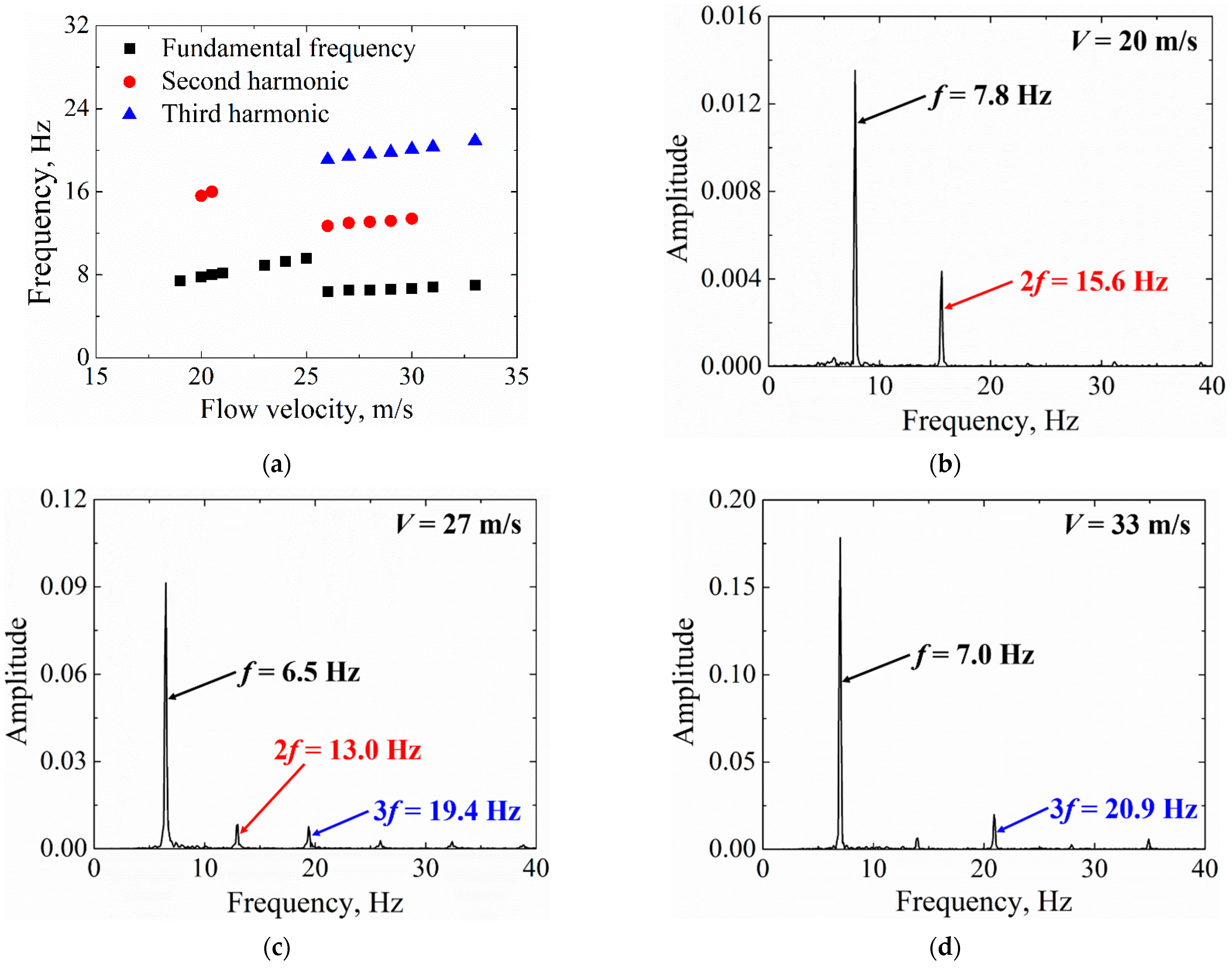
• Significant second order harmonics can sometimes be found in L-LCOs, and their appearance is related to the torsion free-play angle (see Figure 17c and Figure 18c). Additionally, a further increase in the flow velocity seems to result in a disappearance of second order harmonics in L-LCO (see Figure 16c,d).

4.3. Stability of Limit Cycles

Stability analysis is an important tool in the study of nonlinear dynamics. An excitation device consisting of an air pump, conduit, and switch was designed to study the stability of limit cycles. By controlling the switch, the high-pressure air in the air pump can be sprayed onto the model to simulate gust excitation. The amplitudes of acceleration with and without excitation vs. flow velocity are shown in Figure 19a (${\delta }_t=0.165°$ is taken as an example). It is worth noting that the excitation will result in the disappearance of L-LCOs only when the flow velocity is slightly greater than V_L-LCO. Further, time histories of acceleration with excitation when V = 20 m/s and V = 28 m/s are shown in Figure 19b,d, respectively. The responses after excitation remained consistent with the original LCOs, regarded as stable limit cycles. Figure 19c shows the time history of acceleration with excitation when V = 27 m/s. The disappearance of LCO after excitation indicates that this limit cycle was unstable, and the unstable LCO will turn to be stable as the flow velocity increases (i.e., when V ≥ 28 m/s).

5. Conclusions

In this study, an all-movable horizontal tail model with bending and torsion free-plays was designed to investigate the aeroelastic responses induced by multiple free-plays experimentally. The main findings of this paper can be summarized as follows:

• The all-movable horizontal tail with multiple free-plays experienced two independent LCOs, which were induced by bending free-play (S-LCO) and torsion free-play (L-LCO), respectively. Further analyses of the LCOs indicated that the S-LCO mainly contained bending vibration, while the L-LCO contained both bending vibration and torsion vibration.
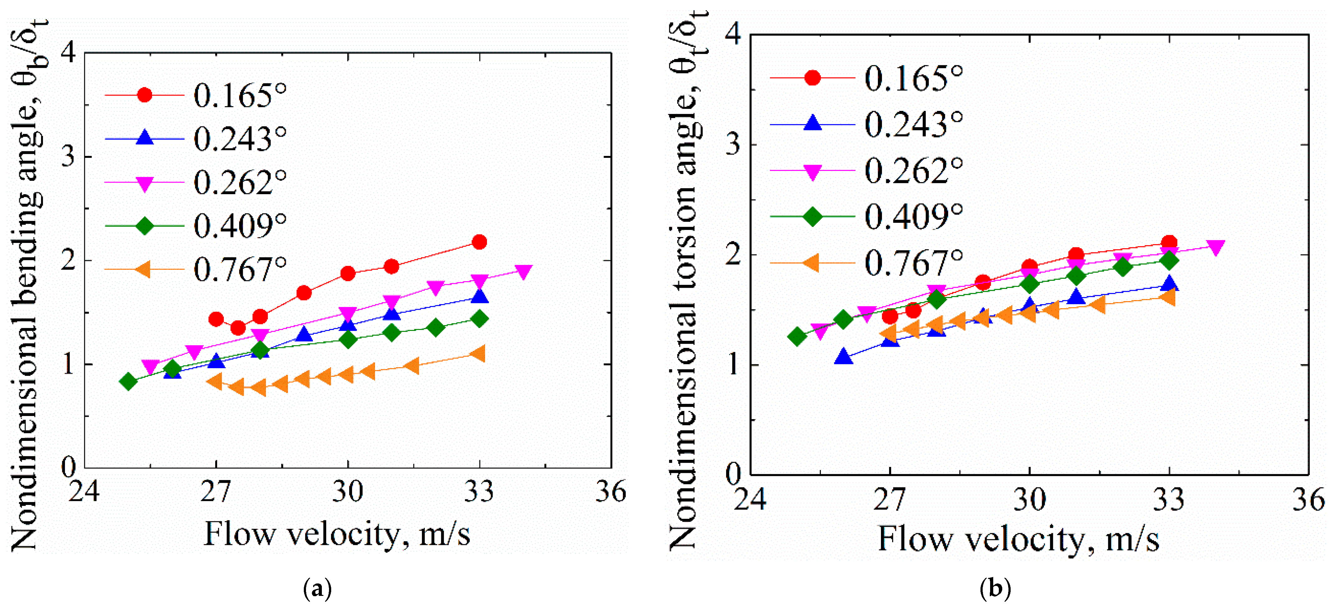
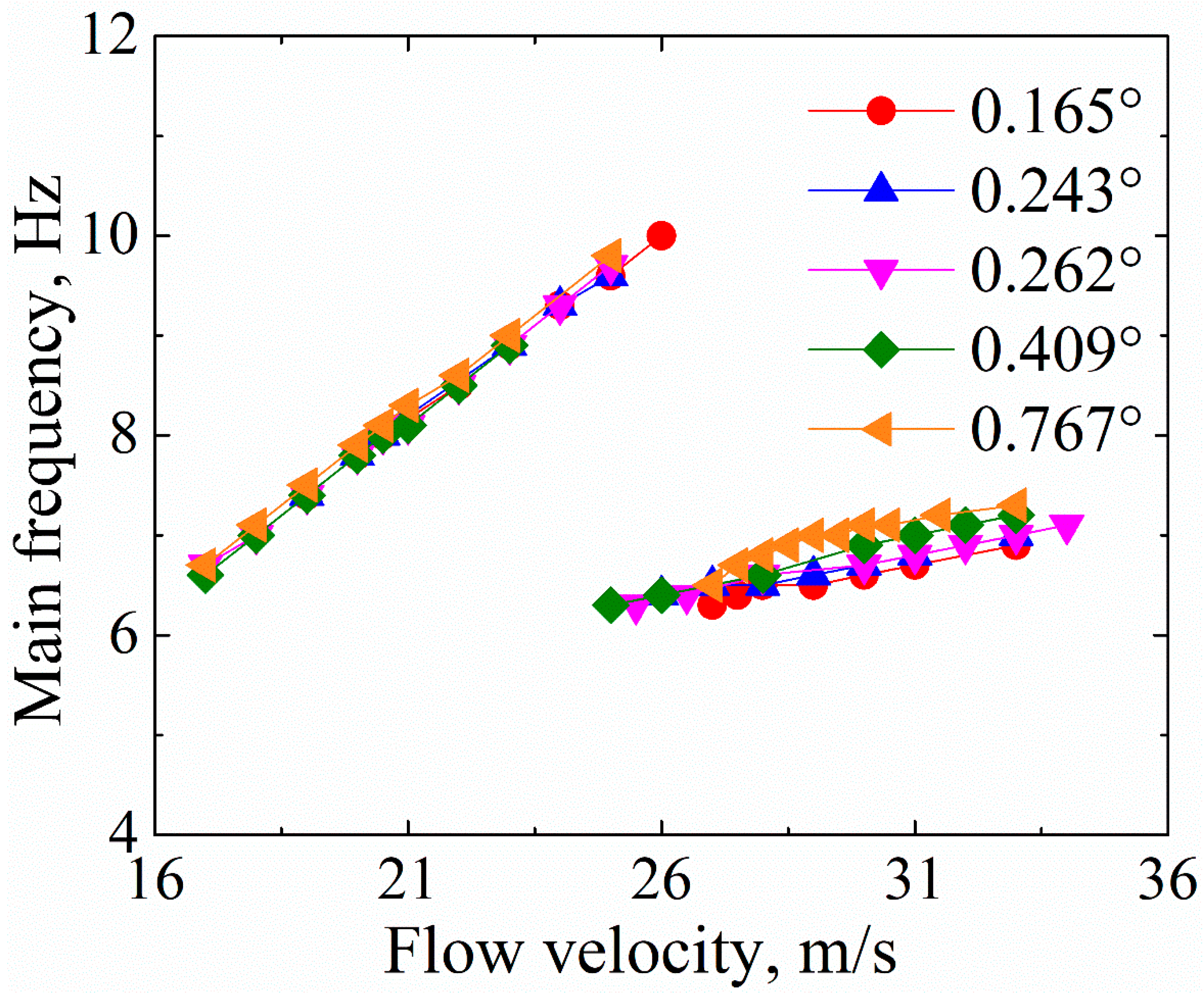
• The torsion free-play angle only affected the characteristics of the L-LCO it triggered, not those of the S-LCO. The amplitude and frequency of the L-LCO increased continuously with the increase in torsion free-play angle and flow velocity.
• High-order harmonics always appeared along with LCOs. It was also found that the characteristics of high-order harmonics were related to the free-play angle and flow velocity.
• The L-LCO was unstable only when the flow velocity was slightly greater than V_L-LCO. Otherwise, the L-LCO was stable.

In conclusion, it was verified experimentally that the all-movable horizontal tail with multiple free-plays exhibited more complex dynamic responses than the single free-play system. Hence, high nonlinearity as a result of multiple free-plays should be considered effectively in the design process, to ensure that the all-movable horizontal tail avoids LCOs within the flight envelope. In addition, these experimental results also provide a significant reference for prediction methods of LCOs induced by multiple free-plays.

References

1. Hilger, J.; Ritter, M.R. Nonlinear Aeroelastic Simulations and Stability Analysis of the Pazy Wing Aeroelastic Benchmark. Aerospace 2021, 8, 308. [Google Scholar] [CrossRef]
2. Kheiri, M. Nonlinear Dynamics of Imperfectly-supported Pipes Conveying Fluid. J. Fluids Struct. 2020, 93, 102850. [Google Scholar] [CrossRef]
3. Yuan, W.; Poirel, D.; Wang, B. Simulations of Pitch–Heave Limit-Cycle Oscillations at a Transitional Reynolds Number. AIAA J. 2013, 51, 1716–1732. [Google Scholar] [CrossRef]
4. Eaton, A.J.; Howcroft, C.; Coetzee, E.B.; Neild, S.A.; Lowenberg, M.H.; Cooper, J.E. Numerical Continuation of Limit Cycle Oscillations and Bifurcations in High-Aspect-Ratio Wings. Aerospace 2018, 5, 78. [Google Scholar] [CrossRef]
5. Sun, Y.; Zhao, D.; Zhu, X. Generation and Mitigation Mechanism Studies of Nonlinear Thermoacoustic Instability in a Modelled Swirling Combustor with a Heat Exchanger. Aerospace 2021, 8, 60. [Google Scholar] [CrossRef]
6. Breitbach, E. Effects of Structural Nonlinearities on Aircraft Vibration and Flutter. In Proceedings of the 45th Structures and Materials AGARD Panel Meeting, AGARD Report 665, Voss, Norway, 26 September 1977. [Google Scholar]
7. Lee, B.H.K.; Price, S.J.; Wong, Y.S. Nonlinear Aeroelastic Analysis of Airfoils: Bifurcation and Chaos. Prog. Aerosp. Sci. 1999, 35, 205–334. [Google Scholar] [CrossRef]
8. Zhang, X.; Kheiri, M.; Xie, W.F. Nonlinear Dynamics and Gust Response of a Two-dimensional Wing. Int. J. Non-Linear Mech. 2020, 123, 103478. [Google Scholar] [CrossRef]
9. Huang, C.; Huang, J.; Song, X.; Zheng, G.; Yang, G. Three Dimensional Aeroelastic Analyses Considering Free-play Nonlinearity Using Computational Fluid Dynamics/Computational Structural Dynamics Coupling. J. Sound Vib. 2021, 494, 115896. [Google Scholar] [CrossRef]
10. Candon, M.; Levinski, O.; Ogawa, H.; Carrese, R.; Marzocca, P. A Nonlinear Signal Processing Framework for Rapid Identification and Diagnosis of Structural Freeplay. Mech. Syst. Signal Process. 2022, 163, 107999. [Google Scholar] [CrossRef]
11. He, H.; Tang, H.; Yu, K.; Li, J.; Yang, N.; Zhang, X. Nonlinear Aeroelastic Analysis of the Folding Fin with Freeplay Under Thermal Environment. Chin. J. Aeronaut. 2020, 33, 2357–2371. [Google Scholar] [CrossRef]
12. Candon, M.; Carrese, R.; Ogawa, H.; Marzocca, P.; Mouser, C.; Levinski, O.; Silva, W.A. Characterization of a 3DOF Aeroelastic System with Freeplay and Aerodynamic Nonlinearities-Part I: Higher-order Spectra. Mech. Syst. Signal Process. 2019, 118, 781–807. [Google Scholar] [CrossRef]
13. Ma, Z.S.; Wang, B.; Zhang, X.; Ding, Q. Nonlinear System Identification of Folding Fins with Freeplay Using Direct Parameter Estimation. Int. J. Aerosp. Eng. 2019, 2019, 3978260. [Google Scholar] [CrossRef]
14. Kholodar, D.B. Nature of Freeplay-induced Aeroelastic Oscillations. J. Aircr. 2014, 51, 571–583. [Google Scholar] [CrossRef]
15. Tian, W.; Gu, Y.; Liu, H.; Wang, X.; Yang, Z.; Li, Y.; Li, P. Nonlinear Aeroservoelastic Analysis of a Supersonic Aircraft with Control Fin Free-play by Component Mode Synthesis Technique. J. Sound Vib. 2021, 493, 115835. [Google Scholar] [CrossRef]
16. Tang, D.; Dowell, E.H. Aeroelastic Response Induced by Free Play, part 2: Theoretical/Experimental Correlation Analysis. AIAA J. 2011, 49, 2543–2554. [Google Scholar] [CrossRef]
17. Wu, Z.; Yang, N.; Yang, C. Identification of Nonlinear Structures by the Conditioned Reverse Path Method. J. Aircr. 2015, 52, 373–386. [Google Scholar] [CrossRef]
18. Hu, P.; Zhao, H.; Xue, L.; Ni, K.; Liu, H. High-fidelity Modeling and Simulation of Flutter/LCO for All-movable Horizontal Tail with Free-play. In Proceedings of the AIAA Atmospheric Flight Mechanics Conference, Portland, OR, USA, 8–11 August 2011. [Google Scholar] [CrossRef]
19. Kim, J.Y.; Kim, K.S.; Lee, I.; Park, Y.K. Transonic Aeroelastic Analysis of All-Movable Wing with Free Play and Viscous Effects. J. Aircr. 2008, 45, 1820–1824. [Google Scholar] [CrossRef]
20. Tang, D.; Dowell, E.H. Computational/Experimental Aeroelastic Study for a Horizontal-Tail Model with Free Play. AIAA J. 2013, 51, 341–352. [Google Scholar] [CrossRef]
21. Ni, K.; Hu, P.; Zhao, H.; Dowell, E.H. Flutter and LCO of an All-movable Horizontal Tail with Freeplay. In Proceedings of the 53rd AIAA/ASME/ASCE/AHS/ASC Structures, Structural Dynamics and Materials Conference, Honolulu, HI, USA, 23–26 April 2012. [Google Scholar] [CrossRef]
22. Arévalo, F.; García-Fogeda, P. Aeroelastic Characteristics of Slender Wing/Bodies with Freeplay Non-Linearities. Proc. Inst. Mech. Eng. Part G J. Aerosp. Eng. 2010, 225, 347–359. [Google Scholar] [CrossRef]
23. Kim, S.H.; Lee, I. Aeroelastic Analysis of a Flexible Airfoil with a Free-play Nonlinearity. J. Sound Vib. 1996, 193, 823–846. [Google Scholar] [CrossRef]
24. Chen, P.C.; Ritz, E.; Lindsley, N. Nonlinear Flutter Analysis for the Scaled F-35 with Horizontal-Tail Free Play. J. Aircr. 2014, 51, 883–889. [Google Scholar] [CrossRef]
25. Chen, P.C.; Lee, D.H. Flight-loads Effects on Horizontal Tail Free-play-induced Limit Cycle Oscillation. J. Aircr. 2008, 45, 478–485. [Google Scholar] [CrossRef]
26. Zhang, X.; Kheiri, M.; Xie, W.F. Aeroservoelasticity of an Airfoil with Parametric Uncertainty and Subjected to Atmospheric Gusts. AIAA J. 2021, 59, 4326–4341. [Google Scholar] [CrossRef]
27. Tian, W.; Yang, Z.; Zhao, T. Nonlinear Aeroelastic Characteristics of an All-movable Fin with Freeplay and Aerodynamic Nonlinearities in Hypersonic Flow. Int. J. Non-Linear Mech. 2019, 116, 123–139. [Google Scholar] [CrossRef]
28. Yuan, W.; Zhang, X.; Poirel, D. Numerical Modelling of Aerodynamic Response to Gust. In Proceedings of the AIAA SciTech Forum, Virtual Event, 11–15 and 19–21 January 2021. [Google Scholar] [CrossRef]
29. Yuan, W.; Sandhu, R.; Poirel, D. Fully Coupled Aeroelastic Analyses of Wing Flutter towards Application to Complex Aircraft Configurations. J. Aerosp. Eng. 2021, 34, 04020117. [Google Scholar] [CrossRef]
30. Di Leone, D.; Lo Balbo, F.; De Gaspari, A.; Ricci, S. Model Updating and Aeroelastic Correlation of a Scaled Wind Tunnel Model for Active Flutter Suppression Test. Aerospace 2021, 8, 334. [Google Scholar] [CrossRef]
31. Afonso, F.; Coelho, M.; Vale, J.; Lau, F.; Suleman, A. On the Design of Aeroelastically Scaled Models of High Aspect-Ratio Wings. Aerospace 2020, 7, 166. [Google Scholar] [CrossRef]
32. Banazadeh, A.; Hajipouzadeh, P. Using Approximate Similitude to Design Dynamic Similar Models. Aerosp. Sci. Technol. 2019, 94, 105375. [Google Scholar] [CrossRef]
33. Zuo, C.; Wei, C.; Ma, J.; Yue, T.; Liu, L.; Shi, Z. Full-Field Displacement Measurements of Helicopter Rotor Blades Using Stereophotogrammetry. Int. J. Aerosp. Eng. 2021, 2021, 8811601. [Google Scholar] [CrossRef]
34. Baqersad, J.; Poozesh, P.; Niezrecki, C.; Avitabile, P. Photogrammetry and Optical Methods in Structural Dynamics-A Review. Mech. Syst. Signal Process. 2017, 86, 17–34. [Google Scholar] [CrossRef]
35. Tavallaeinejad, M.; Salinas, M.F.; Paidoussis, M.P.; Legrand, M.; Kheiri, M.; Botez, R.M. Dynamics of Inverted Flags: Experiments and Comparison with Theory. J. Fluids Struct. 2021, 101, 103199. [Google Scholar] [CrossRef]
Figure 1. Schematic of the all-movable horizontal tail model with multiple free-plays.
Aerospace 10 00434 g001
Figure 2. Details of free-play devices: (a) bending free-play device; (b) torsion free-play device.
Aerospace 10 00434 g002
Figure 3. The all-movable horizontal tail model: (a) design model; (b) manufactured model.
Aerospace 10 00434 g003
Figure 4. Free-plays and angle of attack measures.
Aerospace 10 00434 g004
Figure 5. Free-plays and angle of attack measurements: (a) measurements of marker point-1; (b) measurements of marker point-2.
Aerospace 10 00434 g005
Figure 6. GVT arrangement: (a) model setup; (b) distribution of excitation points.
Aerospace 10 00434 g006
Figure 7. GVT modes of the horizontal tail: (a) the first bending mode; (b) the first torsion mode.
Aerospace 10 00434 g007
Figure 8. Wind tunnel arrangement: (a) model setup; (b) binocular vision measurement system.
Aerospace 10 00434 g008
Figure 9. Time histories for single free-play system at different flow velocities: (a) bending angle (indicated by orange lines); (b) torsion angle (indicated by purple lines).
Aerospace 10 00434 g009
Figure 10. Time histories for δ t = 0.767 ° at different flow velocities: (a) bending angle (indicated by orange lines); (b) torsion angle (indicated by purple lines).
Aerospace 10 00434 g010
Figure 11. Displacement-velocity phase portraits for δ t = 0.767 ° at different flow velocities: (a) bending response (indicated by orange points); (b) torsion response (indicated by purple points).
Aerospace 10 00434 g011
Figure 12. Transient states in a vibration period for δ t = 0.767 ° : (a) S-LCO; (b) L-LCO. Yellow and blue shapes indicate bending and torsion vibration states, respectively.
Aerospace 10 00434 g012
Figure 13. Amplitudes of bending angle and torsion angle at different flow velocities: (a) bending angle; (b) torsion angle.
Aerospace 10 00434 g013
Figure 14. Non-dimensional amplitudes of torsion angle and bending angle at different flow velocities: (a) non-dimensional bending angle; (b) non-dimensional torsion angle.
Aerospace 10 00434 g014
Figure 15. The ratio of torsion angle to bending angle at different flow velocities.
Aerospace 10 00434 g015
Figure 16. Main frequency at different flow velocities.
Aerospace 10 00434 g016
Figure 17. FFT frequency of acceleration response for δ t = 0.767 ° : (a) frequency vs. flow velocity; (b) frequency spectrum at V = 20 m/s; (c) frequency spectrum at V = 27 m/s; and (d) frequency spectrum at V = 33 m/s. The red and blue markers indicate the 2nd and 3rd order harmonics, respectively.
Aerospace 10 00434 g017
Figure 18. FFT frequency of acceleration response for δ t = 0.243 ° : (a) frequency vs. flow velocity; (b) frequency spectrum at V = 20 m/s; (c) frequency spectrum at V = 27 m/s; and (d) frequency spectrum at V = 33 m/s. The red and blue markers indicate the 2nd and 3rd order harmonics, respectively.
Aerospace 10 00434 g018
Figure 19. Acceleration time histories under excitation for δ t = 0.165 ° : (a) amplitude of acceleration vs. flow velocity; (b) acceleration time history at V = 20 m/s; (c) acceleration time history at V = 27 m/s; and (d) acceleration time history at V = 28 m/s.
Aerospace 10 00434 g019