Evaluation of Air Combat Control Ability Based on Eye Movement Indicators and Combination Weighting GRA-TOPSIS

Abstract

At present, expert scoring is mainly used to evaluate the air combat control ability, which is not accurate enough to effectively achieve the desired effect. In order to evaluate air battle managers’ air combat control ability more scientifically and accurately, using eye-tracking technology, a quantitative evaluation model is established based on eye movement indicators. Specifically, the air combat control ability was comprehensively assessed using the GRA-TOPSIS method based on the EW-CRITIC combination weighting. The model innovatively uses eye movement indicators as a vital evaluation basis. Firstly, it puts forth a comprehensive evaluation method by combining GRA with TOPSIS methods, using the EW and CRITIC methods for combined weighting, and giving full play to the advantages of various evaluation methods. Secondly, it not only effectively copes with the problem that the traditional evaluation method is deeply affected by subjectivity but also creatively provides a reasonable means for future training evaluation of air battle managers. Finally, the effectiveness and feasibility of the evaluation model are verified through case analysis.

1. Introduction

As the pilot’s “third wingman”, air battle managers (ABMs) are a vital part of aviation operations. It is worth mentioning that their primary function is to guide the aircraft to reach the designated area, form a favorable situation, and accurately intercept or attack enemy targets. In a sense, air combat control is the continuous command and control process over the aircraft. Moreover, it is an integral part of the aviation combat command. Furthermore, the air combat control ability of ABMs is the cornerstone of air combat victory. More importantly, it conducts an irreplaceable role in overcoming the enemy.

However, how to effectively measure the air combat control ability of ABMs has always been a problem to research. Fowley [1] pointed out that the US military assessed the undergraduate ABMs through simulation training and practical operation and paid more attention to the latter. Luppo et al. [2] summarized the main methods of the ability evaluation of air traffic controllers, including continuous assessment, dedicated assessment, oral examination, and written examination. Picano et al. [3] combed the ability assessment methods of high-risk warfighters from multiple dimensions, such as psychology, intelligence, personality, and physical ability. In daily training, the evaluation of air combat control ability usually adopts the method of expert scoring; that is, experts score each subject by observing the air combat control process. Since the scoring standards vary with each individual, this evaluation method is subjectively affected more. There are often large differences in expert opinions and inaccurate assessments. To identify the weak links in peacetime training and select the best candidates, we must accurately evaluate the air combat control capability of ABMs. Therefore, an effective way to objectively measure air combat control ability is urgently needed.

Eye movement measurement methods are widely used in human–computer interaction, medical security, military training, and other fields [4,5,6]. The US military found that applying eye movement analyses to air force training can significantly improve the training effect. Among the fifteen training subjects of the F-16B, ten used the eye movement measurement system [7]. Using eye-tracking devices, Dubois et al. [8] recorded the gaze patterns of military pilots in simulation tasks and compared them with the correct ones. They found that the trainee pilots spent too much time looking at inboard instruments. Babu et al. [9] estimated the cognitive load of pilots in a military aviation environment by eye-tracking technology. Li et al. [10] found that eye-tracking technology can help flight instructors effectively identify trainee pilots’ inappropriate operational behaviors and improve their monitoring performance. Eye movement measurement can obtain rich, diverse, comprehensive, and objective data compared with observation methods [11]. Hence, to evaluate air combat control ability, we introduced the technique of eye movement measurement. It can quantitatively analyze the air combat control ability of ABMs through relevant eye movement indicators combined with voice notification to avoid the adverse impact of subjective factors on the assessment.

The evaluation process involves the calculation and processing of multiple indicators. As shown in Table 1, standard solutions include Fuzzy Comprehensive Evaluation (FCE), Vlsekriterijumska Optimizacija I Kompromisno Resenje (VIKOR), TODIM, Grey Relation Analysis (GRA), and Technique for Order Preference by Similarity to an Ideal Solution (TOPSIS) methods [12,13,14,15,16]. The abovementioned limitations prevent the comprehensive evaluation of the air combat control capability of ABMs, so the GRA-TOPSIS method is used in this study to address this issue. The TOPSIS method is a classic multi-attribute decision-making model whose central idea is to rank the schemes according to the closeness of the finite number of evaluation objectives to the positive and negative ideal solutions [17]. However, the TOPSIS method also has some defects. It only considers the Euclidean distance between the indicators without taking into account their correlation. Since they are independent components, they cannot accurately capture how the evaluation indication sequence is evolving [16]. Due to the problems mentioned above, the GRA method, which can reflect each project’s closeness from the perspective of curve shape similarity, is introduced to improve it. In order to measure the degree of relationship based on the geometrical characteristic of the lines, the observed values of discrete behaviors of systematic factors are converted into piecewise continuous lines through linear interpolation [18]. Combining the two methods can make up for the defect that the TOPSIS method only calculates the relative distance between indicators but ignores the internal variation laws of the scheme [19]. Hence, we considered using the GRA-TOPSIS model to solve these problems.

Table 1. Comparison of comprehensive evaluation methods.

Methods	Merits	Defects
FCE	1. Be able to make a more scientific, reasonable, and practical quantitative evaluation of the data with fuzzy information 2. The evaluation result is a vector rather than a point value and contains rich information 3. Make qualitative problems quantitative and improve the accuracy and feasibility of evaluation	1. Complex calculation process 2. Strong subjectivity 3. Only consider the main factors and ignore the secondary factors so that the evaluation results are not comprehensive 4. When there are many indicators, the weight vector W does not match the fuzzy matrix R, which is easy to cause failure
VIKOR	1. Considering the maximization of group utility and the minimization of individual regret at the same time, it has high-ranking stability and reliability 2. A compromise scheme with priority can be obtained so that there may be more than one optimal scheme	1. Susceptible to subjective influence 2. The weight coefficient and value of the criterion are required to be determined, which is difficult to achieve in actual decision-making
TODIM	1. Simple calculation process 2. Based on prospect theory, widely used	1. Susceptible to subjective influence 2. It cannot evaluate the situation where the effect value is an interval value
GRA	1. Accurately analyze the trend of the data curve as a scaling curve to measure the shape similarity 2. It is also applicable to the number of samples and the regularity of samples 3. Easy computational and convenient method 4. The quantitative results are consistent with the qualitative analysis results 5. Reduce the loss caused by information asymmetry	1. Strong subjectivity 2. It is difficult to determine the optimal value of some indicators 3. It is necessary to determine the optimal value of each index
TOPSIS	1. Scientific and objective evaluation process 2. There are no strict restrictions on data distribution, sample size, and indicators 3. Simple calculation process 4. It can well depict the comprehensive impact of multiple impact indicators 5. Wide application range	1. The data of each indicator is required, and the selection of quantitative indicators will be difficult 2. It cannot determine the appropriate number of indicators to describe the impact of indicators

In addition, we must empower indicators since we need to create a weighted assessment matrix for the computation procedure. As shown in Table 2, the methods of empowerment are divided into subjective and objective. The former includes Analytic Hierarchy Process (AHP), Decision Alternative Ratia Evaluation System (DARE), Delphi, etc. [20,21,22]. The latter includes Coefficient of Variation (CV), Principal Component Analysis (PCA), Criteria Importance Through Intercriteria Correlation (CRITIC), Entropy Weight (EW), etc. [23,24,25,26]. In order to reduce the subjective influence and obtain more accurate weights, we considered using the EW-CRITIC combination method for objective weighting.

Table 2. Comparison of weighting methods.

Methods	Merits	Defects
AHP	1. Systematic analysis method 2. Simple and practical decision-making method 3. Less quantitative data information required	1. Cannot provide new solutions for decision-making 2. Susceptible to subjective influence 3. When there are too many indicators, the data statistics are extensive, and the weight is difficult to determine 4. The exact solution of eigenvalues and eigenvectors is relatively complex
DARE	1. The calculation process is simple and convenient 2. Make full use of all indicators	1. The scope of application is small, and it is only applicable to problems with obvious comparable relations among the evaluation objects 2. Susceptible to subjective influence
Delphi	1. Convenient evaluation process 2. It is conducive to independent thinking and judgment of experts	1. Strong subjectivity 2. The investigation took quite a long time 3. The investigation conclusion may be close to the median or arithmetic mean
CV	1. The calculation process is simple and convenient 2. Can effectively distinguish various indicators	1. There are certain errors in the calculation results 2. The premise of use is that each indicator is of equal importance, and there are specific requirements for the selection of indicators
PCA	1. No parameter limit 2. It can eliminate the relevant impact between evaluation indicators 3. Reduce the workload of indicator selection	1. Eigenvalue decomposition has some limitations, such as the transformation matrix must be a square matrix 2. When the sign of the factor load of the principal component is positive or negative, the meaning of the comprehensive evaluation function is not clear
CRITIC	1. Comprehensively consider the contrast strength and conflict of indicators 2. Simple and convenient calculation process	1. Requirement of specific normalization formulations and relatively more evident modeling mechanism 2. The dispersion between indicator data is not considered
EW	1. The deviation caused by human factors is avoided 2. The precision is high, which can better explain the results obtained 3. Unbiased, simple, and reliable 4. Modular and user-friendly 5. Produces more divergent coefficient values, hence can better resolve the inherent conflict between the criteria	1. Too sensitive to abnormal data 2. Neglecting the importance of indicators, sometimes the determined indicator weights will be far from the expected results

2. Literature

As shown in Table 3, we sorted the literature using relevant methods in recent years. To select suitable nanoparticles to remit the thermal issues in energy storage systems, Dwivedi et al. [27] adopted the AHP and EW-CRITIC methods to empower them from both subjective and objective aspects, and the GRA-TOPSIS method was used to evaluate, compare, and rank several different alternatives. Because experts’ clustering has been frequently based on their preference similarity, without considering the defect of individual opinion, Chen et al. [28] proposed a two-tiered collective opinion generation framework integrating an expertise structure and risk preference to solve this problem. Cheng et al. [29] used the EW-CRITIC method and TOPSIS model to measure the equilibrium level of urban and rural basic public services (BPS). Gong et al. [30] used the EW-CRITIC method and Ordinary Least Squares (OLS) model to evaluate the urban post-disaster vitality recovery, better representing the spatial characteristics of urban vitality. To promote the sustainable development of the construction industry, Chen et al. [31] solved the problem of Sustainable Building Material Selection (SBMS) in an uncertain environment by developing a comprehensive multi-standard large-group decision-making framework. Additionally, the SBMS was eventually accomplished by the Improved Basic Uncertain Linguistic Information (IBULI)-based TOPSIS method. Weng et al. [32] used the improved EW-CRITIC empowerment and GRA-VIKOR method to select private sector partners for public–private partnership projects and compared the evaluation results with those of traditional GRA, VIKOR, and TOPSIS methods to demonstrate the superiority of this method. Rostamzadeh et al. [33] used the mixed CRITIC-TOPSIS method in the sustainable supply chain risk assessment to effectively manage the enterprise. With the aid of technical and financial factors, Babatunde and Ighravwe [34] employed the CRITIC-TOPSIS mixed fuzzy decision-making model to evaluate the renewable energy system. Chen et al. [35] built a multi-angle Multi-Perspective Multiple-Attribute Decision-Making (MPMADM) framework to provide systematic decision support for enterprises to select the best Third-Party RL Providers (3PRP) and introduced Generalized Comparative Linguistic Expressions (GCLE) for 3PRLP selection, which provided greater flexibility for experts to clarify their evaluation. A model of agricultural machinery selection based on the GRA-TOPSIS method of EW-CRITIC combination weighting was established by Lu et al. [36] to address the problems of insufficient decision-making information and intense subjectivity of index weights in the process of selecting agricultural machinery. Liu et al. [37] used the EW-TOPSIS model to measure the maturity of China’s carbon market. Sakthivel et al. [38] used Fuzzy Analytic Hierarchy Process (FAHP), GRA, and TOPSIS to evaluate the best fuel ratio to select the best mixture between fish and diesel oil. Chen et al. [39] proposed a new perspective to encoding Proportional Hesitant Fuzzy Linguistic Term Sets (PHFLTS) based on the concept of a Proportional Interval T2 Hesitant Fuzzy Set (PIT2HFS). In addition, based on the Hamacher aggregation operators and the andness optimization models, a Proportional Interval T2 Hesitant Fuzzy TOPSIS method was developed to provide linguistic decision-making under uncertainty.

Table 3. Comparison of related studies.

Author	Problem	Weighting Method	Model	Reference
Dwivedi	Select suitable nanoparticles to remit the thermal issues in energy storage systems	AHP EW-CRITIC	GRA-TOPSIS	[27]
Cheng	Measure the equilibrium level of urban and rural basic public services	EW-CRITIC	TOPSIS	[29]
Gong	Evaluate the urban post-disaster vitality recovery	EW-CRITIC	OLS	[30]
Weng	Select private sector partners for public-private partnership projects	EW-CRITIC	GRA-VIKOR	[32]
Rostamzadeh	The risk assessment of a sustainable supply chain	CRITIC	TOPSIS	[33]
Babatundea Ighravweb	Evaluate the renewable energy system	CRITIC	TOPSIS	[34]
Lu	The process of agricultural machinery selection	EW-CRITIC	GRA-TOPSIS	[36]
Liu	Measure the maturity of China’s carbon market	EW	TOPSIS	[37]
Sakthivel	Evaluate the best fuel ratio	FAHP	GRA—TOPSIS	[38]

Currently, most studies on the air combat control ability of ABMs in the military are at the qualitative analysis level. A relatively small number of studies have been conducted on establishing quantitative evaluation models based on eye movement indicators. We established a quantifiable mathematical model based on the relevant eye movement indicators. It conducts a comprehensive and objective evaluation of the air combat control ability based on the combined weighted GRA-TOPSIS method, giving full play to the advantages of various evaluation methods. Through a large number of experiments, it has been proved that the accuracy of the results obtained by eye-tracking technology is greatly improved compared with that obtained by traditional evaluation methods. Moreover, we innovatively introduced the eye-tracking evaluation method into the field of capability evaluation. In addition to providing a new method for evaluating the training of ABMs and further improving the combat training system, it also provides a method for evaluating personnel capabilities in various related fields. This fully overcomes the shortcomings of traditional evaluation methods, such as strong subjectivity, lacking a theoretical basis, and unified evaluation standards.

The remainder of the paper is organized as follows. In Section 2, the evaluation model of air combat control capability is established, and each evaluation indicator is analyzed in detail. Section 3 introduces the evaluation method of air combat control capability. Section 4 describes the experimental setup and example calculation. In Section 5, we summarize our research results and expected future applications.

3. Air Combat Control Ability Evaluation Indicator Modeling

3.1. Indicator System

In air combat, the complex battlefield situation, the changeable enemy aircraft, the uninterrupted threat warning, and the urgent emergency all test the air combat control ability of the ABMs. Based on the characteristics of tight time, heavy tasks, huge intensity, and high precision in the air battlefield environment, we selected indicators such as agility, accuracy, attention, and cognitive load to measure it. This paper follows the principles of scientificity, comprehensiveness, stability, independence, and testability. After consulting a large number of materials [1,2,3,12,13,14,15,16,23,24,25,26,27,28,29,30,31,32,33,34,35,36,37,38,39,40], we conducted on-site research in relevant units, summarized combat training experience, discussed with over twenty experts in the field who are the professors and officers of Air Force, and combined the air combat control process to establish an evaluation indicator system for assessing air combat control ability, as shown in Figure 1.

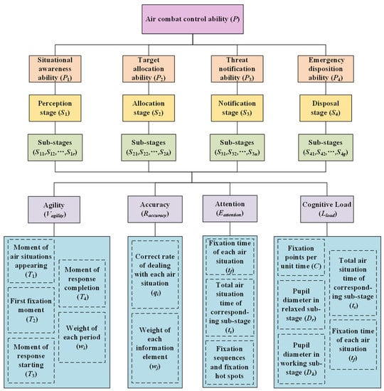
Figure 1. Evaluation indicator system of air combat control ability based on relevant eye movement indicators. The air combat control ability includes situational awareness, target allocation, threat notification, and flying emergency disposition ability. The operation stages corresponding to the four abilities are perception, allocation, notification, and disposal. Due to different tasks being performed in the four stages, different weights correspond to the entire air combat control process. In addition, the four major stages, respectively, include several sub-stages (S_1r, S_2k, S_3u, S_4g), and the corresponding weights of different sub-stages are also different. The values of r, k, u, and g are determined a ccording to the specific combat tasks.

3.2. Indicator Model

In order to present the evaluation indicator model more clearly, we provided a detailed introduction from four aspects: agility, accuracy, attention, and cognitive load. Additionally, we established calculation models for them and analyzed the meaning of each indicator to ensure that our evaluation method was easier to understand. The details are as follows.

(1) Agility

In aviation operations, victory or defeat can often be determined in a matter of seconds, which is why the agility of ABMs in air combat control is vital. We can calculate three indicators of agility according to five sub-indicators: the appearance moment of different aerial situations, the first fixation moment of each aerial situation, the start moment of the response, the finish moment of the response, and the weight of each period. There are three agility indicators in the sub-stage: discovery time, reaction time, and response time to each aerial situation. The weighted sum of each period is used to calculate the total time of air combat control in different sub-stages, and then the agility of air combat control is obtained. The calculation model is as follows:

$$\left\{\begin{array}{l}{V}_{NAagility}=m_N/t_{NAtotal}\\ t_{NAtotal}=w_{NAa}\times t_{NAa}+w_{NAb}\times t_{NAb}+w_{NAc}\times t_{NAc}\\ t_{NAa}=T_{NA2}-T_{NA1}\\ t_{NAb}=T_{NA3}-T_{NA2}\\ t_{NAc}=T_{NA4}-T_{NA3}\\ T_{NA1}<T_{NA2}<T_{NA3}<T_{NA4}\\ 1=w_{NAa}+w_{NAb}+w_{NAc}\\ N=1,2,3,4\\ A=1,2,\cdots ,\infty \end{array}\right.$$

(1)

As shown in Table 4, the relevant indicators in Formula (1) are briefly introduced.

Table 4. Agility evaluation indicators.

Sub-Stage	Indicator	Meaning	Unit
Perception Sub-stages (S1r)	V1ragility	The agility of perceiving critical aerial situations	piece·s−1
	m1	The incident of ABMs’ situational awareness	piece
	t1rtotal, t1ra, t1rb, t1rc	The total perception time of air combat control, the discovery time, reaction time, and perception time to the critical aerial situations	s
	T1r1, T1r2, T1r3, T1r4	The moment of critical aerial situations appearing, the first fixation moment of critical aerial situations, the moment of perception starting, and the moment of perception completing	s
	w1ra, w1rb, w1rc	The weight of each period	%
Allocation Sub-stages (S2k)	V2kagility	The agility in assigning targets	piece·s−1
	m2	The incident of ABMs assigning targets	piece
	t2ktotal, t2ka, t2kb, t2kc	The total time to assign targets, and the detection time, reaction time, and allocation time to the targets	s
	T2k1, T2k2, T2k3, T2k4	The moment of the targets appearing, the first fixation moment of the targets, the moment of allocation starting, and the moment of allocation completing	s
	w2ka, w2kb, w2kc	The weight of each period	%
Notification Sub-stages (S3u)	V3uagility	The agility of threat notification	piece·s−1
	m3	The incident of ABMs reporting the threats	piece
	t3utotal, t3ua, t3ub, t3uc	The total time to report the threats, the detection time, reaction time, and notification time for the threats	s
	T3u1, T3u2, T3u3, T3u4	The moment of the threats appearing, the first fixation moment of the threats, the moment of notification starting, and the moment of notification completing	s
	w3ua, w3ub, w3uc	The weight of each period	%
Disposal Sub-stages (S4g)	V4gagility	The agility of flying emergency disposition	piece·s−1
	m4	The incident of ABMs dealing with flying emergencies	piece
	t4gtotal, t4ga, t4gb, t4gc	The total time to deal with the flying emergencies, the discovery time, reaction time, and disposal time for the flying emergencies	s
	T4g1, T4g2, T4g3, T4g4	The moment of appearance of the flying emergencies, the first fixation moment of flying emergencies, the moment of disposition starting, and the moment of disposition completing	s
	w4ga, w4gb, w4gc	The weight of each period	%

(2) Accuracy

An ABM’s accuracy of air combat control refers to its ability to deal with different aerial situations in controlling aerial combat, including the accuracy of issuing instructions, allocating targets, and reporting information. It can be calculated by weighing the correct rate of dealing with each aerial situation. The calculation model is as follows.

$$\left\{\begin{array}{c}{R}_{MBaccuracy}=\hfill \\ w_{MB1}{q}_{MB1}+w_{MB2}{q}_{MB2}+\cdots +w_{MBn}{q}_{MBn}\hfill \\ q_{MBS}=0,1\hfill \\ 1=w_{MB1}+w_{MB2}+\cdots +w_{MBn}\hfill \\ M=1,2,3,4\hfill \\ i=1,2,\cdots ,n\hfill \\ B=1,2,\cdots ,\infty \hfill \end{array}\right.$$

(2)

As shown in Table 5, the relevant indicators in Formula (2) are briefly introduced.

Table 5. Accuracy evaluation indicators.

Sub-Stage	Indicator	Meaning	Unit
Perception Sub-stages (S1r)	R1raccuracy	The accuracy of perceiving critical aerial situations	%
	q1r1, q1r2, …, q1rn	The correct rate of each information element when the ABMs perceive the critical aerial situations	%
	w1r1, w1r2, …, w1rn	The weight of each information element	%
Allocation Sub-stages (S2k)	R2kaccuracy	The accuracy of assigning targets	%
	q2k1, q2k2, …, q2kn	The correct rate of each allocation scheme when the ABMs assign targets	%
	w2k1, w2k2, …, w2kn	The weight of each allocation scheme	%
Notification Sub-stages (S3u)	R3uaccuracy	The accuracy of threat notification	%
	q3u1, q3u2, …, q3un	The correct rate of each information element when the ABMs report the threats	%
	w3u1, w3u2, …, w3un	The weight of each information element	%
Disposal Sub-stages (S4g)	R4gaccuracy	The accuracy of flying emergency disposition	%
	q4g1, q4g2, …, q4gn	The correct rate of each information element when the ABMs dispose of flying emergencies	%
	w4g1, w4g2, …, w4gn	The weight of each information element	%

(3) Attention

As part of the problem of attention distribution, air combat control refers to the level of attention that ABMs pay to different aerial situations. Excellent ABMs will allocate their limited energy to the key elements in each aerial situation as much as possible. In the actual evaluation, qualitative analysis can be carried out by eye movement indicators, such as fixation hot spots or fixation sequences, and according to the ratio between the fixation time and the total aerial time in each sub-stage, a quantitative calculation may be performed. The calculation model is as follows.

$$\left\{\begin{array}{c}{E}_{\mathit{KFatention}}=t_{\mathit{KFfixation}}/t_{\mathit{KFsum}}\hfill \\ t_{KFsum}=T_{KF6}-T_{KF5}\hfill \\ T_{KF6}>T_{KF5}\hfill \\ K=1,2,3,4\hfill \\ F=1,2,\cdots ,\infty \hfill \end{array}\right.$$

(3)

As shown in Table 6, the relevant indicators in Formula (3) are briefly introduced.

Table 6. Attention evaluation indicators.

Sub-Stage	Indicator	Meaning	Unit
Perception Sub-stages (S1r)	E1rattention	The attention to perceiving critical aerial situations	%
	t1rfixation, t1rsum	The fixation time on the critical aerial situations, the total time of the critical aerial situations appearing	s
	T1r5, T1r6	The appearance moment and the end moment of critical aerial situations	s
Allocation Sub-stages (S2k)	E2kattention	The attention to assigning targets	%
	t2kfixation, t2ksum	The fixation time on the targets, the total allocated time	s
	T2k5, T2k6	The first fixation moment and completion moment of assigning targets	s
Notification Sub-stages (S3u)	E3uattention	The attention to threat notification	%
	t3ufixation, t3usum	The fixation time on threats, total notification time	s
	T3u5, T3u6	The start moment and the end moment of threat notification	s
Disposal Sub-stages (S4g)	E4gattention	The attention to flying emergency disposition	%
	t4gfixation, t4gsum	The fixation time and total disposal time on the flying emergencies	s
	T4g5, T4g6	The appearance moment of the flying emergencies, the completion moment of disposing of flying emergencies	s

(4) Cognitive Load

Cognitive load is the total amount of mental resources information processing generates when a person completes a specific task [41]. During air combat control, the complicated and ever-changing enemy situations can easily cause a large cognitive load on the ABMs. Therefore, cognitive load is essential for evaluating air combat control ability. Privitera et al. [42] pointed out that cognitive load is mainly generated during the subjects’ sustained fixation. The longer the fixation time, the greater the cognitive load. Compared to reading more accessible materials, Henderson et al. [43] found that complex materials significantly increased fixation points. According to the study of Hess et al. [44], the pupil diameter became more extensive when the subjects calculated multiplication problems with increasing difficulty.

Therefore, the cognitive load of the ABMs can be quantitatively solved according to the eye movement indicators, such as the attention to each aerial situation, the number of fixation points per unit time in the corresponding sub-stage, and the pupil diameter difference between the working and relaxing state. The calculation model [45] is as follows:

$$\left\{\begin{array}{c}{L}_{IHload}=\hfill \\ G\times (t_{IHfixation}/t_{IHsum})\times C_{IH}\times (D_{IHpupil-work}-D_{pupil-relax})+f\hfill \\ D_{IHpupil-work}>D_{pupil-relax}\hfill \\ I=1,2,3,4\hfill \\ H=1,2,\cdots ,\infty \hfill \end{array}\right.$$

(4)

In Formula (4), G is the correlation between each eye movement indicator and cognitive load, and f is the deviation factor. Based on 987,179 data points from the experimental records of 85 subjects, Xue et al. [45] obtained G = 0.624, f = 1.891, and demonstrated a high degree of accuracy of the expression through error analysis.

As shown in Table 7, the relevant indicators in Formula (4) are briefly introduced.

Table 7. Cognitive load evaluation indicators.

Sub-Stage	Indicator	Meaning	Unit
Perception Sub-stages (S1r)	L1rload	The cognitive load from critical aerial situations	each·s−1·mm
	t1rfixation, t1rsum	The fixation time on the critical aerial situations, the total time of the critical aerial situations appearing	s
	C1r	The fixation points per unit of time	each·s−1
	D1rpupil-work, Dpupil-relax	The pupil diameter of the left eye in the working and relaxed state	mm
Allocation Sub-stages (S2k)	L2kload	The cognitive load from assigning targets	each·s−1·mm
	t2kfixation, t2ksum	The fixation time on the targets, the total allocated time	s
	C2k	The fixation points per unit of time	each·s−1
	D2kpupil-work, Dpupil-relax	The pupil diameter of the left eye in the working and relaxed state	mm
Notification Sub-stages (S3u)	L3uload	The cognitive load from threat notification	each·s−1·mm
	t3ufixation, t3usum	The fixation time on threats, the total notification time	s
	C3u	The fixation points per unit of time	each·s−1
	D3upupil-work, Dpupil-relax	The pupil diameter of the left eye in the working and relaxed state	mm
Disposal Sub-stages (S4g)	L4gload	The cognitive load from flying emergency disposition	each·s−1·mm
	t4gfixation, t4gsum	The fixation time and total disposal time on the flying emergencies	s
	C4g	The fixation points per unit of time	each·s−1
	D4gpupil-work, Dpupil-relax	The pupil diameter of the left eye in the working and relaxed state	mm

4. Air Combat Control Ability Assessment Method

4.1. EW-CRITIC Combination Weighting

In the EW method, the amount of information contained in each indicator’s entropy value is used to calculate the indicator’s weights, which can fully exploit the inherent laws and information contained in the original data [46]. The CRITIC method comprehensively measures the objective weight based on the contrast strength of the evaluation indicators and the conflict between indicators [47]. However, the number of samples significantly affects the single EW method, and the single CRITIC method does not consider the discreteness between indicators. Therefore, we adopted the EW-CRITIC method, a combination of the EW and CRITIC methods, to compensate for their shortcomings effectively in the combined weighting [48]. The specific calculation steps are as follows [49]:

(1) Form an indicator evaluation matrix. x_ij (i = 1, 2, …, n; j = 1, 2, …, m) represents the value of the jth indicator in the ith plan.

(2) Construct a standardized evaluation matrix. The initial data are normalized, and the processing formula of the positive (benefit type) indicator is

$$y_{ij}=\frac{x_{ij}-\min \left(x_j\right)}{\max \left(x_j\right)-\min \left(x_j\right)}$$

(5)

The processing formula of the reverse (cost type) indicator is

$$y_{ij}=\frac{\max \left(x_j\right)-x_{ij}}{\max \left(x_j\right)-\min \left(x_j\right)}$$

(6)

(3) Determine the indicator entropy weight

Calculate characteristics of the proportion p_ij of the jth indicator in the ith plan

$$p_{ij}=\frac{y_{ij}}{{\displaystyle \sum _{i=1}^n{y}_{ij}}}$$

(7)

Find the information entropy e_j of the jth indicator

$$e_j=-\frac{1}{\ln n}{\displaystyle \sum _{i=1}^n{p}_{ij}\ln p_{ij}}$$

(8)

Calculate the entropy weight w_ej of the jth indicator

$$w_{ej}=\frac{1-e_j}{m-{\displaystyle \sum _{j=1}^m{e}_j}}$$

(9)

(4) The variability of indicators

Expressed in the form of standard deviation

$$\left\{\begin{array}{l}{\overline{y}}_j=\frac{1}{n}{\displaystyle \sum _{i=1}^n{y}_{ij}}\\ S_j=\sqrt{\frac{{\displaystyle \sum _{i=1}^n{\left(y_{ij}-{\overline{y}}_j\right)}^2}}{n-1}}\end{array}\right.$$

(10)

S_j represents the standard deviation of the jth indicator. In the CRITIC method, the standard deviation represents the difference and fluctuation of the internal values of each indicator. The larger the standard deviation is, the more significant the numerical difference of the indicator will be, and the more information can be displayed. Hence, the more muscular the indicator’s evaluation strength is, the more weight it should be assigned.

(5) The conflict of indicators

Represented by the correlation coefficient

$$\left\{\begin{array}{l}{r}_{jk}=\frac{{\displaystyle \sum _{i=1}^n\left(y_{ij}-{\overline{y}}_j\right)\left(y_{ik}-{\overline{y}}_k\right)}}{\sqrt{{\displaystyle \sum _{i=1}^n{\left(y_{ij}-{\overline{y}}_j\right)}^2{\displaystyle \sum _{i=1}^n{\left(y_{ik}-{\overline{y}}_k\right)}^2}}}}\\ R_j={\displaystyle \sum _{k=1}^m\left(1-r_{jk}\right)}\end{array}\right.$$

(11)

r_jk represents the correlation coefficient between the jth evaluation indicator and the kth indicator, and R_j represents the conflict of the jth indicator. The correlation coefficient is used to describe the correlation between indicators. The stronger the correlation with other indicators, the less conflict between the indicators. Moreover, the more the same information is reflected, the more repetitive the evaluation content will be. Therefore, the repetition weakens the evaluation strength of this indicator to a certain extent, and it should be given a lower weight.

(6) Amount of information

$$C_j=S_j\times R_j=S_j{\displaystyle \sum _{k=1}^m\left(1-r_{jk}\right)}$$

(12)

C_j is the amount of information contained in the jth indicator. The larger the value is, the greater the amount of information the indicator will be. Thus, the more vital the relative importance of the indicator, the greater the weight assigned.

(7) Determine the CRITIC weight of the indicators

Calculate the objective weight w_cj of the jth indicator

$$w_{cj}=\frac{C_j}{{\displaystyle \sum _{j=1}^m{C}_j}}$$

(13)

(8) Combination weighting

We adopted the “multiplication” ensemble method to calculate the total weight, which can realize the complementary advantages between the two objective weighting methods of EW-CRITIC. The calculation formula of the comprehensive weight w_j is as follows.

$$w_j=\frac{w_{ej}{w}_{cj}}{{\displaystyle \sum _{j=1}^m{w}_{ej}{w}_{cj}}}$$

(14)

4.2. GRA-TOPSIS

TOPSIS, a simple ranking method in conception and application, attempts to choose alternatives simultaneously with the shortest distance from the positive ideal solution and the farthest distance from the negative ideal solution. The positive ideal solution maximizes the benefit criteria and minimizes the cost criteria, whereas the negative ideal solution maximizes the cost criteria and minimizes the benefit criteria. TOPSIS makes full use of attribute information, provides a cardinal ranking of alternatives, and does not require attribute preferences to be independent [50]. The grey relational theory proposes the grey relational degree analysis for each subsystem. It evaluates the pros and cons of each scheme through the grey relational degree [51]. Considering the above two methods comprehensively, the TOPSIS method can reflect the Euclidean distance between the indicators, and the GRA method can reflect the internal change law of each scheme. By combining the two methods and exerting their advantages simultaneously, the GRA-TOPSIS joint evaluation model is established [52].

(1) Build a weighted evaluation matrix

$$z_{ij}=w_j·y_{ij}$$

(15)

(2) Determine the positive ideal solution Z⁺ and the negative ideal solution Z⁻

$$Z^{+}=\left(z_1^{+},z_2^{+},\cdots ,z_m^{+}\right)$$

(16)

$$Z^{-}=\left(z_1^{-},z_2^{-},\cdots ,z_m^{-}\right)$$

(17)

Among them, z_j⁺ = max(z_1j, z_2j, …, z_nj), z_j⁻ = min(z_1j, z_2j, …, z_nj).

(3) Calculate the Euclidean distance d_i⁺ and d_i⁻ between the evaluation object and the ideal solutions

$$d_i^{+}=\sqrt{{\displaystyle \sum _{j=1}^m{\left(z_j^{+}-z_{ij}\right)}^2}}$$

(18)

$$d_i^{-}=\sqrt{{\displaystyle \sum _{j=1}^m{\left(z_j^{-}-z_{ij}\right)}^2}}$$

(19)

(4) Calculate the grey correlation coefficient r_ij⁺ and r_ij⁻ between the ith ABM and the ideal solution on the jth indicator

$$\left\{\begin{array}{l}{r}_{ij}^{+}=\frac{\underset{i}{\min }\underset{j}{\min }\left|z_j^{+}-z_{ij}\right|+\rho \underset{i}{\max }\underset{j}{\max }\left|z_j^{+}-z_{ij}\right|}{\left|z_j^{+}-z_{ij}\right|+\rho \underset{i}{\max }\underset{j}{\max }\left|z_j^{+}-z_{ij}\right|}=\frac{\rho w_j}{w_j-z_{ij}+\rho w_j}\\ r_{ij}^{-}=\frac{\underset{i}{\min }\underset{j}{\min }\left|z_j^{-}-z_{ij}\right|+\rho \underset{i}{\max }\underset{j}{\max }\left|z_j^{-}-z_{ij}\right|}{\left|z_j^{-}-z_{ij}\right|+\rho \underset{i}{\max }\underset{j}{\max }\left|z_j^{-}-z_{ij}\right|}=\frac{\rho w_j}{z_{ij}+\rho w_j}\end{array}\right.$$

(20)

Among them, ρ ∈ (0, ∞) is called the resolution coefficient. The smaller the ρ, the greater the resolution. The value range of ρ is (0, 1), and the specific value depends on the situation. When ρ ≤ 0.5463, the resolution is the best; generally, ρ = 0.5.

(5) Calculate the grey correlation coefficient matrices R⁺ and R⁻ of each ABM and the ideal solutions Z⁺ and Z⁻

$$\left\{\begin{array}{l}{R}^{+}={\left(r_{ij}^{+}\right)}_{n\times m}\\ R^{-}={\left(r_{ij}^{-}\right)}_{n\times m}\end{array}\right.$$

(21)

(6) Calculate the grey correlation degrees r_i⁺ and r_i⁻ of each ABM with the ideal values Z⁺ and Z⁻

$$\left\{\begin{array}{l}{r}_i^{+}=\frac{1}{m}{\displaystyle \sum _{j=1}^m{r}_{ij}^{+}}\\ r_i^{-}=\frac{1}{m}{\displaystyle \sum _{j=1}^m{r}_{ij}^{-}}\end{array}\right.$$

(22)

(7) Perform dimensionless processing on the Euclidean distances d_i⁺, d_i⁻ and grey relational degrees r_i⁺, r_i⁻, to obtain D_i⁺, D_i⁻, R_i⁺, R_i⁻

$$\left\{\begin{array}{l}{D}_i^{+}=\raisebox{1ex}{$d_i^{+}$}\!\left/ \!\raisebox{-1ex}{$\underset{i}{\max }{d}_i^{+}$}\right.,D_i^{-}=\raisebox{1ex}{$d_i^{-}$}\!\left/ \!\raisebox{-1ex}{$\underset{i}{\max }{d}_i^{-}$}\right.\\ R_i^{+}=\raisebox{1ex}{$r_i^{+}$}\!\left/ \!\raisebox{-1ex}{$\underset{i}{\max }{r}_i^{+}$}\right.,R_i^{-}=\raisebox{1ex}{$r_i^{-}$}\!\left/ \!\raisebox{-1ex}{$\underset{i}{\max }{r}_i^{-}$}\right.\end{array}\right.$$

(23)

(8) Calculate relative closeness T_i

$$T_i=\frac{e_1{D}_i^{-}+e_2{R}_i^{+}}{\left(e_1{D}_i^{-}+e_2{R}_i^{+}\right)+\left(e_1{D}_i^{+}+e_2{R}_i^{-}\right)}$$

(24)

e₁ and e₂ are the degrees of preference of the evaluator, and e₁ + e₂ = 1; generally, e₁ = e₂ = 0.5.

(9) The larger T_i is, the closer the ABMs are to the positive ideal solution. That is, the stronger the air combat control ability of the ith AMB is.

The algorithm flow of the above GRA-TOPSIS model based on EW-CRITIC combination weighting is shown in Figure 2.

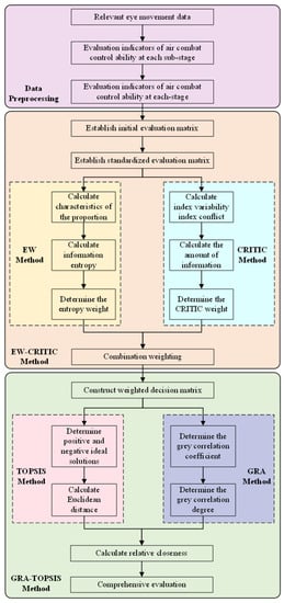
Figure 2. Algorithm flow chart.

Firstly, based on the evaluation indicator model of air combat control ability, the evaluation indicators (agility, accuracy, attention, cognitive load) in each sub-stage of air combat control are calculated according to the relevant eye movements data, such as fixation time, pupil diameter, and fixation points. Secondly, the EW-CRITIC method is used to objectively weigh each sub-stage evaluation indicator and obtain the corresponding indicators’ comprehensive evaluation value in the four stages through the weighted summation. Then, the initial evaluation matrix is normalized to construct a standardized evaluation matrix, and the EW-CRITIC method is used to obtain the weight of each indicator in the standardized evaluation matrix. Finally, a weighted decision matrix is constructed, and the GRA-TOPSIS method is used to determine the positive and negative ideal solutions. In addition, the Euclidean distance, grey correlation coefficient, grey correlation degree, and relative closeness are calculated. Hence, we can obtain a comprehensive ranking and comprehensively evaluate the air combat control ability of the ABMs.

5. Case Analysis of Air Combat Control Ability Evaluation

5.1. Experimental Design

(1) Experimental setup

The experimental subjects were ten ABMs who passed the initial qualification certification, with an average age of 26 years old and a binocular vision above 1.0. They received formal air combat control training and could skillfully complete various air combat control tasks on the command information system. In order to ensure the diversity of the subjects, this study selected the ABMs from different work units, ages, educational levels, working years, and the number of major tasks to participate in the experiment. The basic information about the subjects is shown in Table 8. Before the experiment began, the procedure was introduced to the subjects, who wore the eye tracker for calibration. After the calibration, a 5-minute simulated scenario test was conducted to familiarize the subjects with the eye tracker, and the experiment officially began. Each subject repeated the above process before the experiment started. This experiment is based on the command information system. The subjects simulated air combat control according to the same combat scenario generated by the system. In the experiment, relevant eye movement indicators, as well as the air combat control ability evaluation indicator model, were used to evaluate the air combat control ability.

Table 8. Basic information of subjects.

Subject	Age	Education	Years of Service	Amount of Tasks Executed
X1	33	bachelor	10	19
X2	30	bachelor	7	9
X3	28	bachelor	5	7
X4	29	master	6	17
X5	29	bachelor	6	7
X6	35	bachelor	12	10
X7	31	bachelor	8	11
X8	34	master	11	21
X9	30	master	7	13
X10	26	bachelor	3	8

(2) Experiment apparatus

Experimental equipment includes the command information system and eye-tracking system. The command information system can display the current situations of the enemy in the air based on radar information and provide real-time information support for the ABMs to conduct air combat control. At the same time, it can also generate simulated combat scenarios to assist the ABMs in training. The eye-tracking system consists of eye movement measurement equipment and analysis software. As shown in Figure 3, the eye movement data were measured and collected by the Tobii Pro Glasses 3 eye movement measurement system, which can provide comprehensive eye-tracking data from various viewing angles. Built-in accelerometer, gyroscope, and magnetometer sensors can identify head or eye movements, minimizing the impact of head movements on eye-tracking data. The sampling frequency is 50 Hz or 100 Hz, the shape is the same as ordinary glasses, and the weight is only 76.5 g, which ensures that researchers can obtain the eye movement data of the subjects in the natural state [53]. As shown in Figure 4, the Tobii Pro Lab eye-tracking data analysis software is easy to operate. It can perform qualitative analyses and quantitative calculations on the raw data collected by the Tobii Pro Glasses 3, such as drawing fixation hot spots, fixation sequences, calculating pupil diameter, fixation time, the number of fixation points, the number of visits, the saccade amplitude, etc. [54]. In this experiment, ABMs were equipped with eye-tracking devices to open combat scenarios in the command information system and perform air combat control on our aircraft. After the experiment, the eye movement analysis system was used to analyze and process the collected eye movement data, and the comprehensive evaluation of ABMs’ air combat control ability was conducted based on the indicator model established earlier.

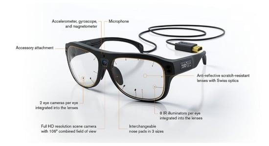
Figure 3. Tobii Pro Glasses 3 eye tracker.

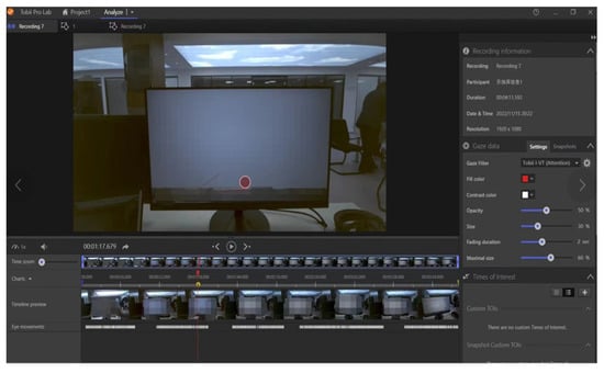
Figure 4. Tobii Pro Lab software operation interface.

(3) Related Eye Movement Indicators

According to the relevant literature [55,56,57,58], we summarized the concept and significance of the leading eye movement indicators in the evaluation indicator model of air combat control ability. As an accurate measurement method, eye-tracking technologies can scientifically and objectively reflect the visual psychological process of the subjects [57]. As shown in Table 9, fixation eye movement indicators can reflect the acquisition and cognitive processing of reading content, and the pupil diameter is closely related to the psychological load of the subjects [58]. Therefore, the use of eye movement indicators can well reflect the professional competence of personnel.

Table 9. Relevant eye movement indicators.

Serial Number	Indicator	Meaning	Unit
1	Fixation time	The duration between the first and last sample makes up a fixation point. It is shown that the subject’s visual focus stays on the observed object for at least 100–200 ms.	s
2	Pupil diameter	The pupil refers to the circular hole with a 2.5–4 mm diameter in the center of the eye’s iris. The changes in pupil diameter can reflect the subjects’ fatigue degree and cognitive load.	mm
3	Fixation hotspot	Each part of the interface is marked with different colors representing the heat to show the attention distribution of the subjects. Generally, the darker the color is, the higher the attention is.	none
4	Fixation sequence	It is a sign to measure the attention distribution of the subjects. Generally, the larger the radius of the fixation point is, the longer the fixation time is.	none
5	First fixation moment	The fixation moment of the first fixation point in the area of interest can be used as an essential indicator to measure perception speed.	s
6	Fixation points per unit of time	During a period, the ratio of the total number of fixation points in the area of interest to the total time can be used to measure the cognitive load of the subjects.	each

(4) Instance overview

Based on the command information system, a combat scenario was constructed to simulate the air combat control process of the ABMs in the actual air combat environment. In this scenario, the red side represents our aircraft (code names are 020 and 021), and the blue side represents the enemy aircraft. The background of the operation is that the enemy aircraft attempted to attack our airport, and we dispatched the air force to intercept them. There are 22 aerial situations in the whole scenario. The situational awareness ability is reflected seven times, the target allocation ability five times, the threat notification ability six times, and the flying emergency disposition ability four times. To make the experimental results more convincing, the combat conditions in each scenario stage do not affect each other.

The timeline of the combat scenario is shown in Figure 5, in which the starting moment of the three enemy aircraft sailing to our airport is set as time K. The time when other events occur is calculated based on time K. As shown in Figure 6, six critical aerial situations in the combat scenario are selected to display the main flow of air combat. Among them, Figure 6a–f, respectively, show the critical aerial situations of K + 3′37″~K + 9′17″, which include tactical deployment, aerial confrontation, destruction, etc.

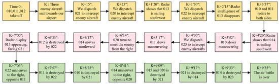
Figure 5. Operational scenario timeline.

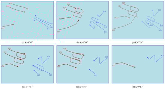
Figure 6. Key operational situation map.

5.2. Instance Calculation

(1) Calculate the evaluation indicators of each sub-stage.

Based on the original data collected by the eye tracker, the agility, accuracy, attention, and cognitive load of the ABMs in each sub-stage of air combat control were calculated by Formulas (1)–(4). As shown in Table 10, the ABMs’ attention to air combat control was taken as an example to analyze. Among them, the abscissa represents the ten ABMs participating in the experiment. The ordinate represents the ABMs’ attention to air combat control in seven perception sub-stages, five allocation sub-stages, six notification sub-stages, and four disposal sub-stages. The other evaluation indicators of air combat control ability are shown in Formula (25).

$$\left\{\begin{array}{l}{V}_{1ragility},R_{1raccuracy},E_{1rattention},L_{1rload}\left(r=1,2,\cdots ,7\right)\\ V_{2kagility},R_{2kaccuracy},E_{2kattention},L_{2kload}\left(k=1,2,\cdots ,5\right)\\ V_{3uagility},R_{3uaccuracy},E_{3uattention},L_{3uload}\left(u=1,2,\cdots ,6\right)\\ V_{4gagility},R_{4gaccuracy},E_{4gattention},L_{4gload}\left(g=1,2,\cdots ,4\right)\end{array}\right.$$

(25)

Table 10. Attention of air combat control.

Attention	X1	X2	X3	X4	X5	X6	X7	X8	X9	X10
E11attention	0.432	0.461	0.207	0.490	0.146	0.882	0.294	0.350	0.325	0.454
E12attention	0.851	0.468	0.260	0.327	0.101	0.166	0.250	0.050	0.122	0.023
E13attention	0.005	0.344	0.031	0.041	0.033	0.006	0.179	0.052	0.096	0.023
E14attention	0.081	0.139	0	0.026	0.040	0.014	0.175	0.010	0.022	0.029
E15attention	0.048	0.324	0.181	0.215	0	0.106	0.093	0.175	0.279	0.207
E16attention	0.013	0.110	0	0.165	0.120	0.018	0.005	0.091	0.066	0.105
E17attention	0.077	0.537	0	0.357	0.063	0.018	0.256	0.291	0	0.123
E21attention	0.157	0.578	0.742	0.192	0.231	0.053	0.595	0.189	0.326	0.123
E22attention	0.070	0.541	0	0.115	0.255	0.179	0.522	0.457	0.426	0.122
E23attention	0.455	0.434	0.272	0.094	0.195	0.064	0.445	0.223	0.354	0.106
E24attention	0.289	0.403	0.233	0.104	0	0.127	0	0.832	0.537	0
E25attention	0.053	0	0.318	0.424	0	0.182	0	0.343	0.604	0
E31attention	0.118	0.369	0.225	0.262	0.304	0.083	0.284	0.247	0.111	0.061
E32attention	0.111	0	0.185	0.325	0.190	0.049	0	0.187	0.200	0.042
E33attention	0.207	0.385	0.163	0.073	0.082	0	0.482	0.222	0.192	0
E34attention	0	0.011	0.170	0.175	0.295	0.084	0.153	0.066	0.068	0.020
E35attention	0.052	0	0.288	0.428	0	0	0.250	0.206	0.317	0.011
E36attention	0.205	0.772	0.189	0.694	0.266	0.020	0.363	0.233	0.257	0
E41attention	0.185	0.625	0.397	0.198	0.419	0.416	0.519	0.502	0.413	0.320
E42attention	0.002	0.380	0.002	0.143	0	0.068	0.057	0	0	0.008
E43attention	0.290	0.358	0.337	0.059	0.283	0.206	0.410	0.276	0.153	0.240
E44attention	0.310	0	0.072	0.423	0	0.010	0.354	0.307	0.415	0.020

(2) The EW-CRITIC method solves the weight of each sub-stage evaluation indicator and constructs a standardized evaluation matrix.

The weights of each evaluation indicator in different sub-stages were calculated by Formulas (5)–(14). The weighted summation of the evaluation indicators in each air combat control sub-stage was performed to obtain the corresponding indicators’ comprehensive evaluation value in the four stages and form an initial evaluation matrix. As shown in Formula (26), taking subject X₁ as an example, E_2attention was selected for analysis and calculation, representing the ABMs’ attention to air combat control in the allocation stage. $E_{21attention},\cdots ,E_{25attention}$ represent the ABMs’ attention to air combat control in five sub-stages of allocation, respectively. $w_{E_{21}},\cdots ,w_{E_{25}}$, respectively, represent the EW-CRITIC combination weight of the ABMs’ attention to air combat control in the five allocation sub-stages.

By using Formulas (5) and (6), the initial evaluation matrix of the comprehensive evaluation indicator system was normalized, eliminating the dimension between indicators to form a standardized evaluation matrix, as shown in Table 11.

$$\begin{array}{l}{E}_{2attention}=w_{E_{21}}\times E_{21atteneion}+w_{E_{22}}\times E_{22atteneion}+w_{E_{23}}\times E_{23atteneion}+w_{E_{24}}\times E_{24atteneion}+w_{E_{25}}\times E_{25atteneion}\\ =0.158\times 0.157+0.127\times 0.070+0.142\times 0.455+0.207\times 0.289+0.367\times 0.053\\ =0.178\end{array}$$

(26)

Table 11. Standardized evaluation matrix of the comprehensive evaluation indicator system.

Indicator	X1	X2	X3	X4	X5	X6	X7	X8	X9	X10
V1guide	0.367	0.056	0.053	0.459	1	0.054	0	0.482	0.350	0.192
V2guide	0.572	0.322	0.515	1	0.067	0.460	0.128	0.622	0.597	0
V3guide	0.585	0.028	0.537	0.212	0	0.428	0.691	1	0.491	0.152
V4guide	0.740	0.510	1	0.599	0	0.526	0.447	0.252	0.069	0.293
R1accuracy	0.467	1	0	0.464	0.224	0.901	0.812	0.583	0.693	0.676
R2accuracy	0.619	0.264	0.520	0	0.627	1	0.144	0.778	0.349	0
R3accuracy	0.881	0.163	0.387	0.185	0	0.396	0.401	0.828	1	0.494
R4accuracy	1	0.372	0.512	0.377	0	0.761	0.898	0.825	0.464	0.835
E1attention	0.557	1	0.037	0.533	0	0.245	0.412	0.200	0.128	0.144
E2attention	0.291	0.582	0.617	0.423	0.106	0.189	0.395	0.837	1	0
E3attention	0.289	0.608	0.639	1	0.472	0.047	0.777	0.568	0.619	0
E4attention	0.520	0.969	0.491	1	0	0.150	0.911	0.643	0.782	0.003
L1load	0.527	0.214	0.342	0.612	0.891	0	0.817	1	0.987	0.703
L2load	0.812	0.128	0	0.916	0.593	1	0.239	0.472	0.053	0.996
L3load	0.874	0.303	0	0.383	0.320	1	0.571	0.928	0.671	0.999
L4load	1	0	0.360	0.986	0.636	0.997	0.475	0.904	0.852	0.981

(3) Build a weighted decision matrix

The weights of each evaluation indicator in the four stages were calculated by Formulas (7)–(14), and the results are shown in Table 12. Among them, w_ej represents the weight obtained by the EW method, w_cj represents the weight obtained by the CRITIC method, and w_j means the combined weight obtained by the EW-CRITIC method. Then, the weighted decision matrix was constructed by Formula (15). The similarities and differences among the three weighting methods can be seen in Figure 7. Among them, the green line, red line, and blue line, respectively, represent the weights calculated for each indicator using the entropy weight method, CRITIC method, and combination weighting method. Additionally, the results obtained by the EW method and the combined weighting method are relatively close, and the changing trends of the weights of the indicators in the three weighting methods are similar. Therefore, we adopted the combination weighting method that combines the advantages of the two methods mentioned above, which can yield more accurate results.

Table 12. Weights of the comprehensive evaluation indicator system.

Weight	V1agility	V2agility	V3agility	V4agility	R1accuracy	R2accuracy	R3accuracy	R4accuracy
wej	0.105	0.064	0.074	0.059	0.040	0.081	0.059	0.038
wcj	0.069	0.051	0.051	0.065	0.061	0.069	0.053	0.054
wj	0.114	0.052	0.059	0.061	0.039	0.088	0.050	0.032
Weight	E1attention	E2attention	E3attention	E4attention	L1load	L2load	L3load	L4load
wej	0.092	0.062	0.055	0.072	0.044	0.076	0.045	0.035
wcj	0.062	0.057	0.064	0.070	0.068	0.083	0.061	0.061
wj	0.090	0.056	0.056	0.080	0.047	0.100	0.043	0.034

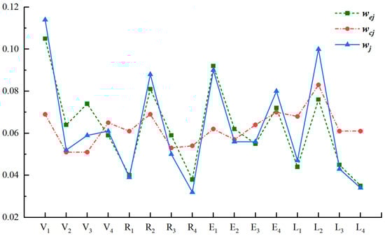
Figure 7. Weights of the comprehensive evaluation indicator system. (4) Comprehensive assessment of ABMs’ air combat control ability using the GRA-TOPSIS method.

The Euclidean distance, grey correlation degree, relative closeness, and total rank are calculated by Formulas (16)–(24), and the results are shown in Table 13. As shown in Figure 8, the horizontal axis represents ten participants, the left vertical axis represents Euclidean distance, the right vertical axis represents gray correlation degree, the orange areas represent d_i⁺, the green areas represent d_i⁻, the blue areas represent r_i⁺, and the pink areas represent r_i⁻. In addition, the relative closeness is comprehensively calculated according to the Euclidean distance and grey correlation obtained from 16 indicators, which objectively reflects the ranking of the air combat control ability of ABMs. The comprehensive ranking of the ten subjects can be seen intuitively in Table 13. On the one hand, the total score of subject X₈ ranks first, with the strongest air combat control ability. On the other hand, the total score of subject X₃ ranks 10th, with the weakest air combat control ability.

Table 13. Comprehensive evaluation results.

Subject	Euclidean Distance		Grey Correlation Degree		Relative Closeness Ti	Comprehensive Ranking
	di+	di−	ri+	ri−
X1	0.123	0.163	0.622	0.460	0.603	2
X2	0.188	0.142	0.524	0.623	0.475	7
X3	0.202	0.112	0.481	0.641	0.423	10
X4	0.144	0.174	0.618	0.514	0.578	3
X5	0.189	0.151	0.471	0.722	0.451	8
X6	0.178	0.161	0.599	0.573	0.524	5
X7	0.184	0.129	0.549	0.544	0.488	6
X8	0.127	0.169	0.665	0.444	0.616	1
X9	0.173	0.141	0.606	0.518	0.526	4
X10	0.207	0.130	0.540	0.663	0.448	9

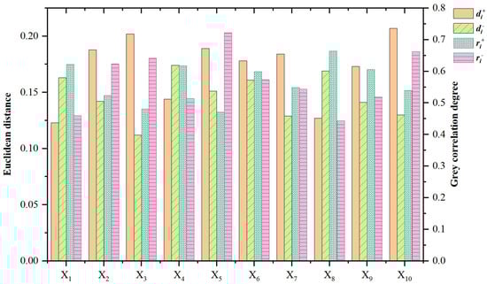
Figure 8. Euclidean distance and grey correlation degree.

Therefore, the comprehensive ranking of the air combat control ability of the ten ABMs can be obtained from the relative closeness T_i of the evaluation indicator system: X₈ > X₁ > X₄ > X₉ > X₆ > X₇ > X₂ > X₅ > X₁₀ > X₃.

According to Table 8, the evaluation results have certain reference values. Among them, X₈, X₁, and X₄ have higher education levels (X₈ and X₄ have master’s degrees), longer working years (X₈ and X₁ have more than 10 years of work experience), more than 15 times of major tasks, solid air combat control theory, and rich experience. In the test, the program was complete, the password was clear, the disposal was appropriate, the key situation could be accurately grasped, and the energy distribution was just right, so it was classified as class A; Among X₉, X₆, X₇, and X₂, only X₉ had a master’s degree. Except for X₆, other ABMs had a working age of 5 to 10 years. On average, they performed no more than 1.5 major tasks every year. They can master the basic theory of air combat control, but there are still some operational deficiencies. In the test, there was a phenomenon of missing air information. The password was not skilled enough, and the grasp of key situations was also lacking. The energy distribution lacked strategy, so it was classified as class B; X₅, X₁₀, and X₃ all have bachelor’s degrees. They have not worked for more than 5 years and have few major tasks to perform. Due to a lack of practice and experience, they cannot skillfully control air combat. In the test, not only was much air information missed, but the key situation could not be perceived in advance. Thus, it was categorized as class C due to poor target allocation strategies, unfamiliar passwords, a sudden special situation that was not dealt with in time, an inability to keep up with the change in air information, heightened emotional tensions, and a high cognitive load.

As shown in Figure 9, the normalization results of various ability indicators of X₈, X₁, and X₄ are generally higher, and the area of the radar map formed is larger. In their air combat control, the procedures are complete, the instructions are clear, the handling is appropriate, the critical aerial situation can be accurately grasped, and the energy distribution is just proper. Therefore, their air combat control ability is stronger. The normalization results of some ability indicators of X₉, X₆, X₇, and X₂ are lower, resulting in the reduced radar map area. In their air combat control, several aerial bits of intelligence are missed, the target allocation strategy is mediocre, the disposal of flying emergencies is not timely, and the energy allocation cannot keep up with the changes in aerial situations. Hence, their air combat control ability is ordinary. The normalization results of various ability indicators of X₅, X₁₀, and X₃ are much lower, and the radar map area is smaller. In their air combat control, they miss much aerial intelligence and cannot perceive critical aerial situations in advance. They are unfamiliar with instructions, untimely deal with the flying emergency, and have a high cognitive load. Therefore, their air combat control ability is poorer.

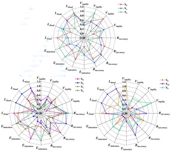
Figure 9. Comparison of normalized results of various indicators of air combat control ability.

As shown in Figure 10, to further verify the validity of the comprehensive evaluation results, the fixation hot spots and fixation sequences of three ABMs, X₃, X₇, and X₈, are compared in the air combat control from K + 6′33″ to K + 7′06″. This period is the sub-stage in which the aerial situation is the most complex in the entire operational scenario and can best reflect the air combat control ability of the ABMs. In addition, the darker the color and the larger the fixation areas are, the higher the attention level of the subjects. We used the eye movement view to visualize the subjects’ attention allocation strategy, thereby measuring the strength of the subjects’ air combat control ability. It can be found that the X₃ spread his attention across all aircraft and even paid attention to many meaningless areas. His fixation point sequence was chaotic and lacked logic, and he did not pay enough attention to most fixation points. Hence, the comprehensive evaluation of air combat control ability ranks 10th. X₇ focused on 015, 010, and 020, but this sub-stage’s most significant aerial situations are 015, 011, and 022. X₇ paid attention to useless aerial situations and did not optimally allocate energy. His fixation point sequence lacked order, but most fixation points are fixed for a long time, so the comprehensive evaluation of air combat control ability ranks 6th. X₈ focused on 015, 011, and 022. At the same time, he considered other aerial situations, and the energy distribution was reasonable. The fixation point sequence was well-organized, and he paid attention to most fixation points. The saccade strategy adopts an efficient top-down method [59], so the comprehensive evaluation of air combat control ability ranks first.

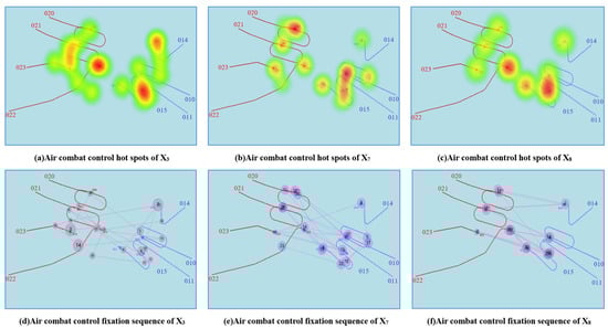
Figure 10. Air combat control eye movement view.

Table 14 shows the comprehensive scores and rankings of participants when selecting different preference coefficients. Additionally, the different colors in Figure 11 correspond to different preference coefficients, reflecting the impact of changes in preference coefficients on the comprehensive scores. From them, we can find that the difference in comprehensive scores obtained by different preference coefficients is small, and the changing trend is basically consistent. Therefore, the change in preference coefficient has little impact on the evaluation results. To reduce the influence of the preference coefficient on comprehensive evaluation as much as possible and balance the advantages and disadvantages of various methods, we selected the comprehensive score at e₁ = 0.5 as the evaluation basis of this paper.

Table 14. Sensitivity analysis of the preference coefficient.

No.	e1	Tscore										Rank
		X1	X2	X3	X4	X5	X6	X7	X8	X9	X10
1	0	0.595	0.477	0.469	0.566	0.414	0.532	0.523	0.619	0.559	0.449	X8 > X1 > X4 > X9 > X6 > X7 > X2 > X3 > X10 > X5
2	0.1	0.596	0.477	0.465	0.569	0.422	0.530	0.516	0.618	0.553	0.444	X8 > X1 > X4 > X9 > X6 > X7 > X2 > X3 > X10 > X5
3	0.2	0.598	0.477	0.461	0.571	0.429	0.529	0.509	0.618	0.546	0.439	X8 > X1 > X4 > X9 > X6 > X7 > X2 > X3 > X10 > X5
4	0.3	0.599	0.476	0.457	0.573	0.437	0.527	0.502	0.617	0.539	0.433	X8 > X1 > X4 > X9 > X6 > X7 > X2 > X3 > X5 > X10
5	0.4	0.601	0.476	0.453	0.576	0.444	0.526	0.495	0.616	0.533	0.428	X8 > X1 > X4 > X9 > X6 > X7 > X2 > X3 > X5 > X10
6	0.5	0.603	0.476	0.448	0.578	0.451	0.524	0.488	0.616	0.526	0.423	X8 > X1 > X4 > X9 > X6 > X7 > X2 > X5 > X3 > X10
7	0.6	0.604	0.475	0.444	0.581	0.459	0.523	0.482	0.615	0.519	0.418	X8 > X1 > X4 > X6 > X9 > X7 > X2 > X5 > X3 > X10
8	0.7	0.606	0.474	0.44	0.583	0.466	0.522	0.475	0.614	0.513	0.413	X8 > X1 > X4 > X6 > X9 > X7 > X2 > X5 > X3 > X10
9	0.8	0.608	0.474	0.436	0.585	0.473	0.520	0.468	0.613	0.506	0.408	X8 > X1 > X4 > X6 > X9 > X2 > X5 > X7 > X3 > X10
10	0.9	0.609	0.474	0.432	0.588	0.480	0.519	0.462	0.613	0.499	0.403	X8 > X1 > X4 > X6 > X9 > X5 > X2 > X7 > X3 > X10
11	1.0	0.611	0.473	0.428	0.590	0.487	0.518	0.455	0.612	0.493	0.398	X8 > X1 > X4 > X6 > X9 > X5 > X2 > X7 > X3 > X10

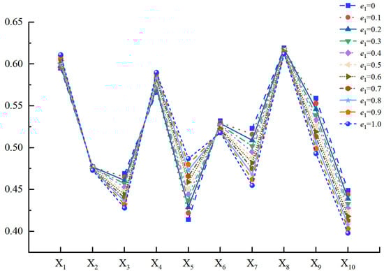
Figure 11. Comparison of comprehensive scores of different preference coefficients.

As shown in Table 15 and Figure 12, it is not difficult to find that the comprehensive evaluation results obtained by different methods are basically the same. The personnel ranking of class A and class C has a small change, while the personnel ranking of class B has a relatively large change. However, according to Table 10 and the daily training performance of ABMs, we can see that the evaluation method selected in this study is the most appropriate and accurate for evaluating personnel’s ability.

Table 15. Comparative analysis of the methods.

No.	Subjects	EW-TOPSIS		CRITIC- GRA		EW-CRITIC -TOPSIS		EW-GRA- TOPSIS		CRITIC -GRA- TOPSIS		EW-CRITIC -GRA- TOPSIS
		Analysis Results	Rank	Analysis Results	Rank	Analysis Results	Rank	Analysis Results	Rank	Analysis Results	Rank	Analysis Results	Rank
1	X1	0.531	2	0.467	2	0.569	2	0.603	2	0.602	2	0.603	2
2	X2	0.460	5	0.394	8	0.431	7	0.480	7	0.458	8	0.476	7
3	X3	0.344	10	0.406	7	0.387	9	0.436	8	0.463	7	0.448	9
4	X4	0.489	4	0.464	3	0.548	3	0.571	3	0.569	3	0.578	3
5	X5	0.387	8	0.354	10	0.444	6	0.435	10	0.412	10	0.451	8
6	X6	0.433	7	0.451	5	0.475	4	0.517	5	0.524	5	0.524	5
7	X7	0.453	6	0.412	6	0.413	8	0.498	6	0.510	6	0.488	6
8	X8	0.593	1	0.500	1	0.571	1	0.626	1	0.625	1	0.616	1
9	X9	0.491	3	0.455	4	0.450	5	0.542	4	0.543	4	0.526	4
10	X10	0.359	9	0.361	9	0.358	10	0.435	9	0.421	9	0.423	10

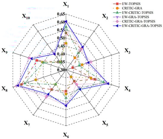
Figure 12. Comparative analysis of the methods.

6. Conclusions

We established an evaluation model of air combat control ability based on objective eye movement indicators. After calculating each evaluation indicator, the GRA-TOPSIS method based on EW-CRITIC combination weighting was used to comprehensively evaluate ABMs’ air combat control ability. The method covers four aspects and a total of 16 indicators, which can effectively avoid the adverse effects of subjective evaluation and obtain more accurate evaluation results.

The data in this study are from the actual data measured in the experiment. In this experiment, the eye movement patterns of the ABMs with better and those with poorer evaluations differ. The former has more fixation points, faster saccade speed, greater attention, and lower cognitive load. In the daily training, we can learn from the eye movement patterns of the outstanding personnel and use the eye tracker to measure their eye movement defects. Moreover, we can evaluate their air combat control process in time, cultivate scientific saccade habits in the early stage of training, and improve training efficiency. In addition, the evaluation method adopted in this study has the advantages of simple test procedures, scientific data collection, accurate evaluation results, etc., and can provide a reference for the professional ability evaluation of personnel in other fields so that it is no longer limited to performance analysis or subjective judgment. However, a more comprehensive and efficient evaluation of personnel capabilities can be conducted through eye movement, Electroencephalograph (EEG), Electromyogram (EMG), and other physiological measurement methods [60]. Finally, this research can be applied to talent selection. Establishing an appropriate eye movement indictor system and objectively measuring the subject’s professional ability according to the measured eye movement data can provide an effective channel for decisionmakers or policymakers to select talents and assess ranking.

Pros: Firstly, the calculation results of the proposed method are accurate. Combining the four methods gives full play to the greatest advantage and can effectively measure the air combat control capability of ABMs. Secondly, the calculation process is simple, and the evaluation results can be obtained fast. Finally, the proposed method can be widely used in various capacity assessment areas.

Cons: Firstly, this model only applies to situations where the air information at each stage is independent. When they are affected by each other, more factors need to be considered, and more complex and accurate models need to be used to calculate. Secondly, due to the particularity of the tested population, only ten ABMs joined the experiment. The weight calculated by the EW-CRITIC method will vary, and more reliable results may be obtained as the number of samples increases. In addition, this experiment is based on the simulated combat scenario of the command information system. If the data can be collected during the guidance of the actual aircraft, the results will be more convincing. Finally, our comprehensive evaluation system of air combat control ability lacks saccade indicators and needs further improvement. Further research will refine the evaluation indicator system, improve the evaluation indicator model, and use more accurate algorithms to optimize the comprehensive evaluation method.

References

- Fowley, J.W. Undergraduate Air Battle Manager Training: Prepared to Achieve Combat Mission Ready; Air Command and Staff College, Distance Learning, Air University Maxwell AFB United States: Montgomery, AL, USA, 2016. [Google Scholar]
- Luppo, A.; Rudnenko, V. Competence assessment of air traffic control personnel. Proceedings Natl. Aviat. Univ. 2012, 2, 47–50. [Google Scholar] [CrossRef]
- Picano, J.J.; Roland, R.R.; Williams, T.J.; Bartone, P.T. Assessment of elite operational personnel. In Handbook of Military Psychology; Springer: Berlin/Heidelberg, Germany, 2017; pp. 277–289. [Google Scholar]
- Majaranta, P.; Bulling, A. Eye Tracking and Eye-Based Human-Computer Interaction; Advances in Physiological Computing; Springer: Berlin/Heidelberg, Germany, 2014; pp. 39–65. [Google Scholar]
- Brunyé, T.T.; Drew, T.; Weaver, D.L.; Elmore, J.G. A review of eye-tracking for understanding and improving diagnostic interpretation. Cogn. Res. Princ. Implic. 2019, 4, 7. [Google Scholar] [CrossRef] [PubMed]
- Moore, L.J.; Vine, S.J.; Smith, A.N.; Smith, S.J.; Wilson, M.R. Quiet eye training improves small arms maritime marksmanship. Mil. Psychol. 2014, 26, 355–365. [Google Scholar] [CrossRef]
- Wetzel, P.A.; Anderson, G.M.; Barelka, B.A. Instructor use of eye position based feedback for pilot training. Hum. Factors Ergon. Soc. 1998, 2, 59. [Google Scholar] [CrossRef]
- Dubois, E.; Blättler, C.; Camachon, C.; Hurter, C. Eye movements data processing for ab initio military pilot training. In Proceedings of the International Conference on Intelligent Decision Technologies, Algarve, Portugal, 21–23 June 2017; pp. 125–135. [Google Scholar]
- Babu, M.D.; Jeevitha Shree, D.V.; Prabhakar, G.; Saluja, K.P.S.; Pashilkar, A.; Biswas, P. Estimating pilots’ cognitive load from ocular parameters through simulation and in-flight studies. J. Eye Mov. Res. 2019, 12. [Google Scholar] [CrossRef]
- Li, W.-C.; Jakubowski, J.; Braithwaite, G.; Jingyi, Z. Did you see what your trainee pilot is seeing? Integrated eye tracker in the simulator to improve instructors’ monitoring performance. In Eye-Tracking in Aviation, Proceedings of the 1st International Workshop (ETA-VI 2020), ISAE-SUPAERO, Toulouse, France, 17 March 2020; Université de Toulouse; Institute of Cartography and Geoinformation (IKG), ETH Zurich: Zurich, Switzerland, 2020; pp. 39–46. [Google Scholar]
- Van Gompel, R.P. Eye Movements: A Window on Mind and Brain; Elsevier: Amsterdam, The Netherlands, 2007. [Google Scholar]
- Zhao, Y.; Zhang, C.; Wang, Y.; Lin, H. Shear-related roughness classification and strength model of natural rock joint based on fuzzy comprehensive evaluation. Int. J. Rock Mech. Min. Sci. 2021, 137, 104550. [Google Scholar] [CrossRef]
- Mardani, A.; Zavadskas, E.K.; Govindan, K.; Senin, A.A.; Jusoh, A. VIKOR technique: A systematic review of the state of the art literature on methodologies and applications. Sustainability 2016, 8, 37. [Google Scholar] [CrossRef]
- Llamazares, B. An analysis of the generalized TODIM method. Eur. J. Oper. Res. 2018, 269, 1041–1049. [Google Scholar] [CrossRef]
- Jana, C.; Pal, M. A dynamical hybrid method to design decision making process based on GRA approach for multiple attributes problem. Eng. Appl. Artif. Intell. 2021, 100, 104203. [Google Scholar] [CrossRef]
- Papathanasiou, J.; Ploskas, N. Topsis. In Multiple Criteria Decision Aid; Springer: Berlin/Heidelberg, Germany, 2018; pp. 1–30. [Google Scholar]
- Vavrek, R. Evaluation of the Impact of Selected Weighting Methods on the Results of the TOPSIS Technique. Int. J. Inf. Technol. Decis. Mak. 2019, 18, 1821–1843. [Google Scholar] [CrossRef]
- Liu, S.; Yang, Y.; Cao, Y.; Xie, N. A summary on the research of GRA models. Grey Syst. Theory Appl. 2013, 3, 7–15. [Google Scholar] [CrossRef]
- Liu, D.; Qi, X.; Fu, Q.; Li, M.; Zhu, W.; Zhang, L.; Faiz, M.A.; Khan, M.I.; Li, T.; Cui, S. A resilience evaluation method for a combined regional agricultural water and soil resource system based on Weighted Mahalanobis distance and a Gray-TOPSIS model. J. Clean. Prod. 2019, 229, 667–679. [Google Scholar] [CrossRef]
- Podvezko, V. Application of AHP technique. J. Bus. Econ. Manag. 2009, 10, 181–189. [Google Scholar] [CrossRef]
- Xiang, C.; Yin, L. Study on the rural ecotourism resource evaluation system. Environ. Technol. Innov. 2020, 20, 101131. [Google Scholar] [CrossRef]
- Dalkey, N.C. Delphi. In An Introduction to Technological Forecasting; Routledge: London, UK, 2018; pp. 25–30. [Google Scholar]
- Faber, D.S.; Korn, H. Applicability of the coefficient of variation method for analyzing synaptic plasticity. Biophys. J. 1991, 60, 1288–1294. [Google Scholar] [CrossRef]
- Abdi, H.; Williams, L.J. Principal component analysis. Wiley Interdiscip. Rev. Comput. Stat. 2010, 2, 433–459. [Google Scholar] [CrossRef]
- Diakoulaki, D.; Mavrotas, G.; Papayannakis, L. Determining objective weights in multiple criteria problems: The critic method. Comput. Oper. Res. 1995, 22, 763–770. [Google Scholar] [CrossRef]
- Zhu, Y.; Tian, D.; Yan, F. Effectiveness of entropy weight method in decision-making. Math. Probl. Engine-Ering 2020, 2020, 1–5. [Google Scholar] [CrossRef]
- Dwivedi, A.; Kumar, A.; Goel, V. Selection of nanoparticles for battery thermal management system using integrated multiple criteria decision-making approach. Int. J. Energy Res. 2022, 46, 22558–22584. [Google Scholar] [CrossRef]
- Chen, Z.S.; Zhang, X.; Rodríguez, R.M.; Pedrycz, W.; Martínez, L.; Miroslaw, J.S. Expertise-structure and risk-appetite-integrated two-tiered collective opinion generation framework for large-scale group decision making. IEEE Trans. Fuzzy Syst. 2022, 30, 5496–5510. [Google Scholar] [CrossRef]
- Cheng, K.; Liu, S. Does Urbanization Promote the Urban–Rural Equalization of Basic Public Services? Evidence from Prefectural Cities in China. Evid. Prefect. Cities China 2023, 1–15. [Google Scholar] [CrossRef]
- Gong, H.; Wang, X.; Wang, Z.; Liu, Z.; Li, Q.; Zhang, Y. How Did the Built Environment Affect Urban Vibrancy? A Big Data Approach to Post-Disaster Revitalization Assessment. Int. J. Environ. Res. Public Health 2022, 19, 12178. [Google Scholar] [CrossRef]
- Chen, Z.S.; Yang, L.L.; Chin, K.S.; Yang, Y.; Pedrycz, W.; Chang, J.P.; Luis, M.; Mirosław, J.S. Sustainable building material selection: An integrated multi-criteria large group decision making framework. Appl. Soft Comput. 2021, 113, 107903. [Google Scholar] [CrossRef]
- Weng, X.; Yang, S. Private-Sector Partner Selection for Public-Private Partnership Projects Based on Improved CRI-TIC-EMW Weight and GRA-VIKOR Method. Discret. Dyn. Nat. Soc. 2022, 1–10. [Google Scholar] [CrossRef]
- Rostamzadeh, R.; Ghorabaee, M.K.; Govindan, K.; Esmaeili, A.; Nobar, H.B.K. Evaluation of sustainable supply chain risk management using an integrated fuzzy TOPSIS-CRITIC approach. J. Clean. Prod. 2018, 175, 651–669. [Google Scholar] [CrossRef]
- Babatunde, M.; Ighravwe, D. A CRITIC-TOPSIS framework for hybrid renewable energy systems evaluation under techno-economic requirements. J. Proj. Manag. 2019, 4, 109–126. [Google Scholar] [CrossRef]
- Chen, Z.S.; Zhang, X.; Govindan, K.; Wang, X.J. Third-party reverse logistics provider selection: A computational semantic a-nalysis-based multi-perspective multi-attributedecision-making approach. Expert Syst. Appl. 2021, 166, 114051. [Google Scholar] [CrossRef]
- Lu, H.; Zhao, Y.; Zhou, X.; Wei, Z. Selection of agricultural machinery based on improved CRITIC-entropy weight and GRA-TOPSIS method. Processes 2022, 10, 266. [Google Scholar] [CrossRef]
- Liu, X.; Zhou, X.; Zhu, B.; He, K.; Wang, P. Measuring the maturity of carbon market in China: An entropy-based TOPSIS approach. J. Clean. Prod. 2019, 229, 94–103. [Google Scholar] [CrossRef]
- Sakthivel, G.; Ilangkumaran, M.; Nagarajan, G.; Priyadharshini, G.V.; Kumar, S.D.; Kumar, S.S.; Suresh, K.S.; Selvan, G.T.; Thilakavel, T. Multi-criteria decision modelling approach for biodiesel blend selection based on GRA–TOPSIS analysis. Int. J. Ambient. Energy 2014, 35, 139–154. [Google Scholar] [CrossRef]
- Chen, Z.-S.; Yang, Y.; Wang, X.-J.; Chin, K.-S.; Tsui, K.-L. Fostering linguistic decision-making under uncertainty: A proportional in-terval type-2 hesitant fuzzy TOPSIS approach based on Hamacher aggregation operators and andness optimization models. Inf. Sci. 2019, 500, 229–258. [Google Scholar] [CrossRef]
- Tian, J.; Wang, B.; Guo, R.; Wang, Z.; Cao, K.; Wang, X. Adversarial Attacks and Defenses for Deep-Learning-Based Unmanned Aerial Vehicles. IEEE Internet Things J. 2022, 9, 22399–22409. [Google Scholar] [CrossRef]
- Sweller, J. Cognitive load during problem-solving: Effects on learning. CognitiveScience 1988, 12, 257–285. [Google Scholar] [CrossRef]
- Privitera, C.M.; Stark, L.W. Algorithms for defining visual regions of interest: Comparison with eye fixations. Trans. Pattern Anal. Mach. Intell. 2000, 22, 970–982. [Google Scholar] [CrossRef]
- Henderson, J.M.; Ferreira, F. Effects of foveal processing difficulty on the perceptual span in reading: Implications for attention and eye movement control. J. Exp. Psychol. Learn. Mem. Cogn. 1990, 16, 417. [Google Scholar] [CrossRef]
- Hess, E.H.; Polt, J.M. Pupil size in relation to mental activity during simple problem solving. Science 1964, 143, 1190–1192. [Google Scholar] [CrossRef]
- Xue, Y.F.; Li, Z.W. Research on online learning cognitive load quantitative model based on eye-tracking technology. Mod. Educ. Technol. 2019, 29, 59–65. [Google Scholar]
- Kumar, R.; Singh, S.; Bilga, P.S.; Jatin; Singh, J.; Singh, S.; Scutaru, M.-L. Revealing the benefits of entropy weights method for multi-objective optimization in machining operations: A critical review. J. Mater. Res. Technol. 2021, 10, 1471–1492. [Google Scholar] [CrossRef]
- Žižović, M.; Miljković, B.; Marinković, D. Objective methods for determining criteria weight coefficients: A modification of the CRITIC method. Decis. Mak. Appl. Manag. Eng. 2020, 3, 149–161. [Google Scholar] [CrossRef]
- Yin, J.; Du, X.; Yuan, H.; Ji, M.; Yang, X.; Tian, S.; Wang, Q.; Liang, Y. TOPSIS Power Quality Comprehensive Assessment Based on A Combination Weighting Method. In Proceedings of the 2021 IEEE 5th Conference on Energy Internet and Energy System Integration (EI2), Taiyuan, China, 22–25 October 2021; pp. 1303–1307. [Google Scholar]
- Wang, J.; Wang, Y. Analysis on Influencing Factors of Financial Risk in China Media Industry Based on Entropy-critic Method and XGBoost. Acad. J. Bus. Manag. 2022, 4, 102–106. [Google Scholar]
- Behzadian, M.; Otaghsara, S.K.; Yazdani, M.; Ignatius, J. A state-of-the-art survey of TOPSIS applications. Expert Syst. Appl. 2012, 39, 13051–13069. [Google Scholar] [CrossRef]
- Wei, G.W. GRA method for multiple attribute decision making with incomplete weight information in intuitionistic fuzzy setting. Knowl. Based Syst. 2010, 23, 243–247. [Google Scholar] [CrossRef]
- Kirubakaran, B.; Ilangkumaran, M. Selection of optimum maintenance strategy based on FAHP integrated with GRA–TOPSIS. Ann. Oper. Res. 2016, 245, 285–313. [Google Scholar] [CrossRef]
- Bishop, R.; Rutyna, M. Eye Tracking Innovation for Aviation Research. J. New Bus. Ideas Trends 2021, 19, 1–7. [Google Scholar]
- Thibeault, M.; Jesteen, M.; Beitman, A. Improved Accuracy Test Method for Mobile Eye Tracking in Usability Scenarios. In Proceedings of the Human Factors and Ergonomics Society Annual Meeting, Seattle, DC, USA, 28 October–1 November 2019; Volume 63, pp. 2226–2230. [Google Scholar]
- Steindorf, L.; Rummel, J. Do your eyes give you away? A validation study of eye-movement measures was used as indicators for mindless reading. Behav. Res. Methods 2020, 52, 162–176. [Google Scholar] [CrossRef]
- Joseph, A.W.; Murugesh, R. Potential eye tracking metrics and indicators to measure cognitive load in human-computer interaction research. J. Sci. Res. 2020, 64, 168–175. [Google Scholar] [CrossRef]
- Greef, T.; Lafeber, H.; Oostendorp, H.; Jasper, L. Eye movement as indicators of mental workload to trigger adaptive automation. In Proceedings of the International Conference on Foundations of Augmented Cognition, San Diego, CA, USA, 19–24 July 2009; pp. 219–228. [Google Scholar]
- Meghanathan, R.N.; van Leeuwen, C.; Nikolaev, A.R. Fixation duration surpasses pupil size as a measure of memory load in free viewing. Front. Hum. Neurosci. 2015, 8, 1063. [Google Scholar] [CrossRef]
- DeAngelus, M.; Pelz, J.B. Top-down control of eye movements: Yarbus revisited. Vis. Cogn. 2009, 17, 790–811. [Google Scholar] [CrossRef]
- Kramer, A.F. Physiological metrics of mental workload: A review of recent progress. Mult. Task Perform. 2020, 279–328. [Google Scholar]
Disclaimer/Publisher’s Note: The statements, opinions and data contained in all publications are solely those of the individual author(s) and contributor(s) and not of MDPI and/or the editor(s). MDPI and/or the editor(s) disclaim responsibility for any injury to people or property resulting from any ideas, methods, instructions or products referred to in the content. |
© 2023 by the authors. Licensee MDPI, Basel, Switzerland. This article is an open access article distributed under the terms and conditions of the Creative Commons Attribution (CC BY) license (https://creativecommons.org/licenses/by/4.0/).