Article

Machine Learning and IoT Trends for Intelligent Prediction of Aircraft Wing Anti-Icing System Temperature

by
E. S. Abdelghany
1,2,*,
Mohamed B. Farghaly
3,
Mishari Metab Almalki
4,
H. H. Sarhan
5 and
Mohamed El-Sayed M. Essa
6,*
1
Mechanical Power Department, Faculty of Engineering, Al-Baha University, Al-Baha P.O. Box 1988, Saudi Arabia
2
Aeronautical Engineering Department, Institute of Aviation Engineering and Technology (I.A.E.T), Egyptian Aviation Academy, Imbaba Airport, Giza 12815, Egypt
3
Mechanical Engineering Department, Faculty of Engineering, Fayoum University, El-Fayoum 63514, Egypt
4
Department of Electrical Engineering, Faculty of Engineering, Al-Baha University, Al-Baha P.O. Box 1988, Saudi Arabia
5
Mechanical Engineering Department, Faculty of Engineering, Port Said University, Port Said 42526, Egypt
6
Electrical Power and Machines Department, Institute of Aviation Engineering and Technology (I.A.E.T), Egyptian Aviation Academy, Imbaba Airport, Giza 12815, Egypt
*
Authors to whom correspondence should be addressed.
Aerospace 2023, 10(8), 676; https://doi.org/10.3390/aerospace10080676
Submission received: 30 April 2023 / Revised: 22 June 2023 / Accepted: 25 July 2023 / Published: 29 July 2023
(This article belongs to the Special Issue Machine Learning for Aeronautics)

Abstract

:
Airplane manufacturers are frequently faced with formidable challenges to improving both aircraft performance and customer safety. Ice accumulation on the wings of aircraft is one of the challenges, which could result in major accidents and a reduction in aerodynamic performance. Anti-icing systems, which use the hot bleed airflow from the engine compressor, are considered one of the most significant solutions utilized in aircraft applications to prevent ice accumulation. In the current study, a novel approach based on machine learning (ML) and the Internet of Things (IoT) is proposed to predict the thermal performance characteristics of a partial span wing anti-icing system constructed using the NACA 23014 airfoil section. To verify the proposed strategy, the obtained results are compared with those obtained using computational ANSYS 2019 software. An artificial neural network (ANN) is used to build a forecasting model of wing temperature based on experimental data and computational fluid dynamics (CFD) data. In addition, the ThingSpeak platform is applied in this article to realize the concept of the IoT, collect the measured data, and publish the data in a private channel. Different performance metrics, namely, mean square error (MSE), maximum relative error (MAE), and absolute variance ( R 2 ), are used to evaluate the prediction model. Based on the performance indices, the results prove the efficiency of the proposed approach based on ANN and the IoT in designing a forecasting model to predict the wing temperature compared to the numerical CFD method, which consumes a lot of time and requires high-speed simulation devices. Therefore, it is suggested that the ANN-IoT approach be applied in aviation.

1. Introduction

Aviation icing is a common occurrence that arises when super-cooled droplets that may be present in clouds at air temperatures below freezing are caught on the wings, engine inlets, and other parts of the aircraft during flight. Ice accumulation on aircraft components can have major effects on the aircraft’s weight and aerodynamic performance. Ice accumulation has a major effect on the aircraft’s aerodynamic forces, and can increase the drag by 40% and decrease lift by 30% [1,2,3,4,5,6,7]. Many accidents and incidents occurred due to ice accumulation, as stated in a report on U.S. inflight icing [8]. Systems to protect against the accumulation of ice can be placed into two categories: anti-icing systems and de-icing systems. Before entering conditions that can lead to icing, anti-icing mechanisms are activated and are intended to stop ice formation while continuously providing energy. Conversely, de-icing systems are usually used to remove ice that regularly accumulates to a considerable thickness [7,9,10,11,12]. Anti-icing bleed air technology is widely used in the aircraft industry [13,14]. Generally, the anti-icing system of the aircraft uses a piccolo tube installed at the wing leading edge and receives the hot bleed air from the intermediate stages of the engine’s compressor to heat the wing surfaces. The hot bleed airflow discharges from the holes of the piccolo tube at a certain angle with high-velocity jets that impinge on the leading edge of the wing’s inner surface, which is defined as the part of the wing that first contacts the air, and, thereby, transfers heat to the metal skin. Next, heat conduction through the metal skin from the inner surface of the wing to the wing outer surface results in the wing outer surface (LE) remaining hot enough to prevent ice accumulation [15,16,17].
Many researchers have investigated geometric and airflow factors to increase anti-icing system performance. In [18], a computational anti-icing model with a full-span model (FSM) is examined to show how the flow develops inside the wing piccolo tube, and a computational anti-icing model with a partial-span model (PSM) is investigated to estimate the performance of the hot air system. The results show that a good agreement between computational results and experimental data was obtained. In [19], an airfoil section with an electro-thermal system of ice protection is investigated, and a mathematical model technique is proposed to analyze mass and heat transmission over wet and dry surface regions.
In [20], a computational model of the three-dimensional segment of a wing with thermal anti-icing (piccolo-type) bays leading into the leading edge of the wing is presented. This model simulated the integrated external and internal thermal flow with heat conductivity through the wing’s solid skin using the NS Fluent software 2019 as a solver. It investigated the (CFD-derived) model under several flight conditions, hot air jet conditions of the piccolo tube inlet, and shape modifications. In [21], a numerical investigation was carried out of the heat and flow transfer properties of the impinging hot air jets on the aircraft’s wing at the surface of the leading edge. This study is grounded in real-world engineering applications, particularly for a UAV flying through areas with severe icing conditions as it climbs to a mid–high altitudes. Two models are constructed with many anti-icing parameters, such as the geometry of the piccolo tube, the structure of holes on the piccolo tube, the spacing between the leading edge and the piccolo tube, and the angle of the holes. Experimental work was carried out by the authors of [22] to cool a semicircular concave surface with impingement cooling. It was observed that the wall jet thickness and the rate of stagnation transfer of heat are both influenced by the distance between the nozzle exit and the target surfaces. In [23], a review of correlations of heat transfer was carried out. In order to assess how well the correlations applied to the piccolo tube of the anti-icing system, they were later included in the LEWICE program. The results were compared quantitatively to examine the results on a considered piccolo tube anti-icing system. In [24], 2D and 3D numerical models of the NACA 2412 airfoil wing section are investigated with an anti-icing bleed air system. The numerical investigation was executed for a constant Mach number of about 0.3 and a bleed airflow pressure and temperature of 90,000 Pa and 453 K, respectively. Other parameters, including the spacing and number of jets, and distance between the piccolo tube and the wing inner surface at the leading edge, were varied. Based on previous research, this study predicted the thermal effectiveness of the wing anti-icing system with the flow parameters and geometric shape of the wing anti-icing model. It investigated some of the parameters, such as the suitable organization of hot bleed air jets along the piccolo tube, the impingement angle (α) of hot air jets ensuing from the piccolo tube, the horizontal distance (H) between the inner surface of the wing and the piccolo tube, and the air mass flow rate of the hot jets.
The technology of deep learning (DL) has been used in many different applications, including smart homes, banking, marketing, airlines, and the aviation field [25,26,27,28,29,30,31,32,33,34,35]. In addition, DL has been used to improve the results of simulation software, controllers, and forecasting models. Recently, researchers have been interested in exploiting this approach to improve the performance of CFD-based simulations and build an accurate and robust prediction model.
It is worth noting that one of the classic problems in the field of heat transfer is the analysis of natural convection in different spaces, such as containers. In [25], two different methods were used to analyze the convection resulting from a heat source in a can, namely, ANN and CFD. An accurate design of an expert system for predicting the time required for convergence and the number of iterations based on CFD and ANNs is presented in [26]. The introduced expert system is able to build a distinct prediction model for the required convergence time and the number of iterations of a CFD analyzer. In [28], a combination of CFD and soft computing techniques was used to design a model to predict the 3D flow variables in curved channels based on ANN and support vectors. In addition, support vector machines (SVM) were designed with CFD to estimate the velocity variables and flow depth in a 60-degree curve [27]. ANNs with wavelet packet transform (WPT) were used to design a model to predict the accumulation of layers of ice on the airfoil surface [28]. This combination has also been used in the design of cold room parameters [29]. The study includes an evaluation of the model performance. In [30], a model using ANNs was presented for the prediction of the accumulation of ice particles on the surface for different types of ailerons, which, based on the results of the numerical experiments, performed well. The results of the numerical experiment were obtained using the foam solver tool for four different ailerons. In [31], a good CFD-based method is presented for constructing a model that simulates ice on the plane using a reduced model. In addition, ANNs have been used as methods to improve CFD efficiency [32]. ANNs have also been used in designing other models for other applications—for example, they have been proposed to implement a model for the sugar crystallization process [33]. In [34], a model is presented to predict the accumulation of ice on aircraft based on the Stack AutoEncoder (SAE) and the Deep Belief Network (DBN). The networks were built based on samples that were collected using the numerical calculation of ice [34]. In addition, an integrated CFD and ANN approach has been applied to build an improved model to forecast the cavitation volume and real performance of a propeller under various physical and geometrical characteristics [35].
Through the previous discussion, we can see that ANNs have been used efficiently in improving the performance of CFD-based approaches for several different case studies. In addition, ANNs have been used in other applications, for example, to improve the performance of controllers in aircraft and hybrid electric vehicles [36,37]. As a result of the emergence of Industry 4.0 and its close connection with the IoT, researchers are interested in exploiting the IoT and applying it in many applications, such as BMS, economics, management, aviation, and many other fields [38,39,40,41,42,43,44,45,46]. For example, the IoT and ANNs were combined to predict, control, and observe the temperature, humidity, and other parameters for a building management system [38].
The ThingSpeak analytics platform was developed for realizing IoT systems for different applications [39,40,41,42]. For example, ThingSpeak has been used to monitor the number of people in a library [39] and, in combination with an Arduino UNO to monitor an environmental system [40]. It has also been applied to the monitoring of humidity and temperature in a room in real time [41]. A Matlab-based analysis combined with ThingSpeak was used to build a monitoring and sensing system for different environmental parameters, including temperature, heat, light intensity, humidity, rain-sensing, barometric pressure, and air quality [42]. CFD is combined with the IoT to simulate changes in temperature in a greenhouse and execute real-time analysis and implement an intelligent temperature cooling control in the greenhouse [43]. The use of the IoT is proposed for carrying out augmented-reality-enhanced maintenance of aircraft on the ground [44]. In addition, the IoT is used to implement minimization of power consumption in batteries for aviation applications [45]. An energy-efficient smart home was created based on IoT technology [46].
It is known that the design of modern aircraft depends on three important stages: theoretical results, experimental testing, and computational simulation [3,4,8,9,11]. As a result, CFD models are being utilized in aviation on a wide scale [12,16,17]. When using CFD approaches, accuracy is required in selecting many parameters in order to obtain successful and acceptable results, as the computational time for the program to complete the simulation depends greatly on the correct selection of these parameters [16,17]. As a result of the time consumed in adjusting the parameters of the CFD model, as well as the difficulty in making accurate adjustments and the need for the program to have high-speed computers to implement the simulation, due to the large number of cells and grids needed to increase the accuracy, CFD is both time and resource consuming. Therefore, one of the aims of this work was to present a modern and innovative method to improve the results of CFD simulation programs.
Based on the above discussion of previous research, this paper presents the application of ANNs with the possibility of monitoring the system temperature using IoT technology in order to design a system that can predict the temperature in an aircraft wing anti-icing system. In addition, the performance of CFD simulation software can be improved by training different ANNs using data collected from the CFD simulation. The aims of the paper can be summarized as follows:
  • Build an accurate model of an aircraft wing anti-icing system;
  • Estimate the heat transfer performance of aircraft wing anti-icing system based on CFD;
  • Evaluate the results of CFD simulations based on different criteria;
  • Design an intelligent ANN model to predict heat transfer based on experimental data and CFD data;
  • Compared the CFD model and ANN model based on different evaluation tests;
  • Monitor the temperature of an aircraft wing anti-icing system using the IoT.

2. Numerical Validation and Verification

It is well known in the field of aircraft that experimental testing is used to estimate the heat transfer performance of aircraft wing anti-icing systems under different flow conditions and geometric parameters. However, this process is very laborious and costs more than numerical methods, such as the CFD approach. CFD-based techniques have become an important tool for supporting, developing, optimizing, verifying, innovating, and, specifically, validating procedures [47,48,49]. In this research, one of the objectives is to estimate the heat transfer performance of an aircraft wing anti-icing system using a CFD-based approach and then improve the approach through the use of ANNs. Figure 1 shows the schematic of an aircraft wing anti-icing system using a piccolo tube. The design optimization of this system is a complex effort because of the huge number of geometric parameters and airflow (internal and external) factors that affect the performance of the anti-icing system. The computational simulation applied in this investigation consisted of three phases (Figure 2). The CFD investigation was initiated during the preprocessing phase of geometry arrangement and grid mesh generation. The model geometry was created by the Design Modeler (DM) 2019 software program and the meshing grid was generated using ANSYS MESH®. The second phase was the generation of the computational solution using the ANSYS® 2019 software and the Finite-Volume Approach. The final stage is the post-processing stage, in which the thermal characteristics of the wing anti-icing system are investigated. Using the CFD model, pressure contours, velocity contours, heat flux contours, streamline contours, temperature contours, and the distribution of temperature on the aircraft wing surface are investigated.

2.1. Anti-Icing Model Geometry

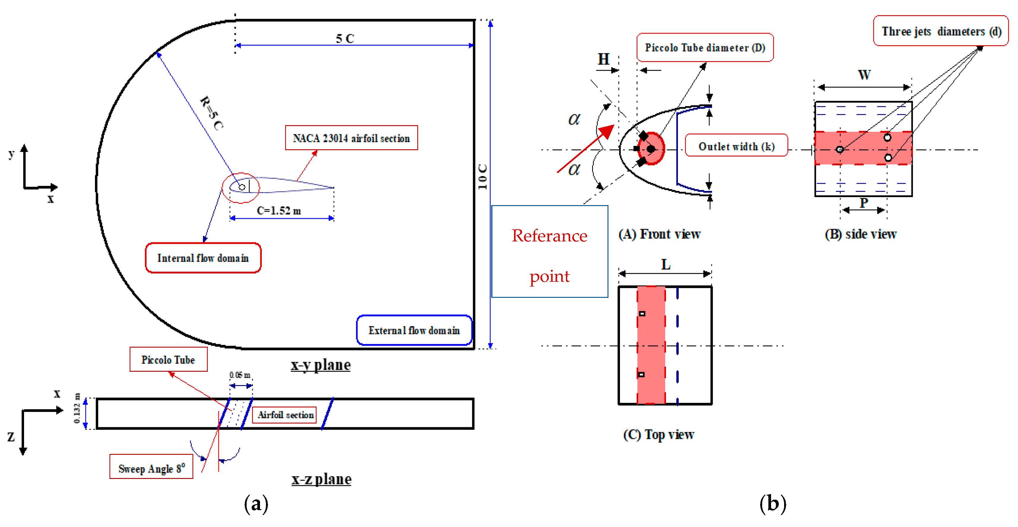
The wing anti-icing system with a NACA 23014 airfoil section is investigated through experiments testing as described in [23]. The experimental results are verified and validated using a CFD-based model based on the same wing anti-icing system design. The anti-icing system is solved numerically using the computational heat transfer method (CHT). The technique of conjugate heat transfer was used to solve three physical domains; first, the external airflow domain composed of the gas phase (atmospheric air), second, the compressible internal flow domain with hot air jets, and third, thermal conduction in the airfoil skin from the interior surface of the wing leading edge to the runback flow on the external surface of the wing (Figure 3). Figure 3a shows the three physical domain dimensions used in the computation (x-y plane and x-z plane). Illustrated is a wing anti-icing system with a NACA 23014 section with a chord (C) length of about 1.52 m. For the x-y plane, the external domain has a half-circular shape with a radius of five times the chord length and a rectangular shape with dimensions of ten times and five times the chord length. For the x-z plane, the wing anti-icing system computational domain has a span length of 0.132 m and a swept angle of 8 deg. The internal domain length (L) is 0.05 m.
Three views of the internal flow domain with all dimension parameters are shown in Figure 3b. The front view presents the internal domain showing dimensions parameters such as the piccolo tube diameter (D) of 0.038 m, the horizontal distance on the center line of the piccolo tube between the wall of the piccolo tube and the point of reference on the inner surface of the wing leading edge (H) of 0.00901 m, the outlet area height (k) of 0.001 m, and jet angles (α) of 45 degrees. The intersection of the piccolo tube center line and the inner surface at the leading edge of the wing is taken as the defined reference point. The side view presents the internal domain showing dimensions parameters such as the diameter (d) of the three jets of 0.00132, the width of the internal flow domain (W) of 0.132 m, and the pitch distance between two columns of jets (P) of 0.066 m. The top view presents the length of the internal flow domain (L). A piccolo with three rows of jets is investigated using an appropriate periodic condition. In the computational internal flow domain, each row of jets is reduced to a single inlet jet.
One of the three rows of jets in the piccolo tube has a jet angle (α) of 0 degrees and is called jet 1. The other two rows of jets in the piccolo tube have jet angles (α) of +45 and −45 degrees and are called jet 2 and jet 3, respectively, as shown in Figure 3b.

2.2. Boundary Conditions of Computational Domain and Solver Settings

The external and internal flow domains of the aircraft wing anti-icing system with boundary conditions are shown in Figure 4. The values for the boundary conditions for the validation model used in this study are the same as those given in [23] (Table 1). The internal flow domain mass flow ( m ˙ ), and temperature for each jet hot air inlet are selected to be equal to 0.327 g/s and 449.82 K, respectively. The liner walls are set as adiabatic walls and the wall of the piccolo tube is set to a constant temperature of about 449.82 K. In addition, the outlet of the internal flow domain is set as zero-gauge pressure. Moreover, the external flow domain, inlet flow velocity, temperature, density, and dynamic viscosity are selected to be equal to 59.16 m/s, 268.21 K, 0.9031 kg/m3, and 1.692 × 10⁻⁵ Ns/m2, respectively. The inlet flow of the angle of attack (AOA) is set to 3 degrees. An opening boundary is set on the down and up surfaces and zero-gauge pressure is set for the outlet flow surface. An open boundary condition describes boundaries in contact with a large volume of fluid. Fluid can both enter and leave the domain on boundaries with this type of condition. An open boundary is also a boundary that doesn’t completely enclose the domain but lets it extend to infinity in at least one direction. In this study, both the external domain and the internal domain are air. Aluminum is used for the material of the solid wing, and it is investigated via fluid–solid interfaces between hot flow, cold flow, and the solid wing to allow the transfer of heat flux.
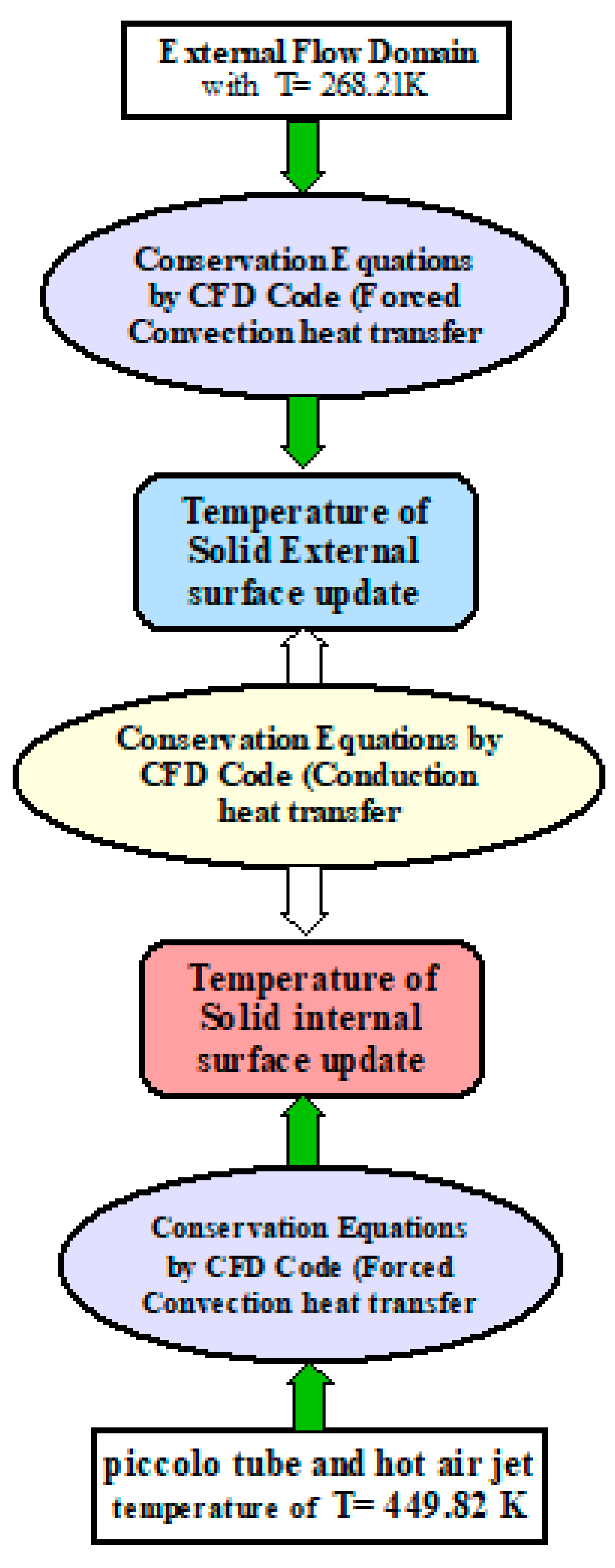
Figure 5 illustrates the flow chart for the anti-icing model simulation. The anti-icing model splits the physical domain into three domains: (1) the external domain with a temperature of 268.21 K, which is solved by conservation equations (CFD Model Forced Convection) to update the temperature of the solid external surface; (2) the internal domain with a temperature of 449.82 K, which is solved by the same method to update the temperature of the solid internal surface; and (3) the solid domain, which conducts heat from the internal surface of the leading edge to the runback flow on the wing external surface.

2.3. Computational Domain Discretization

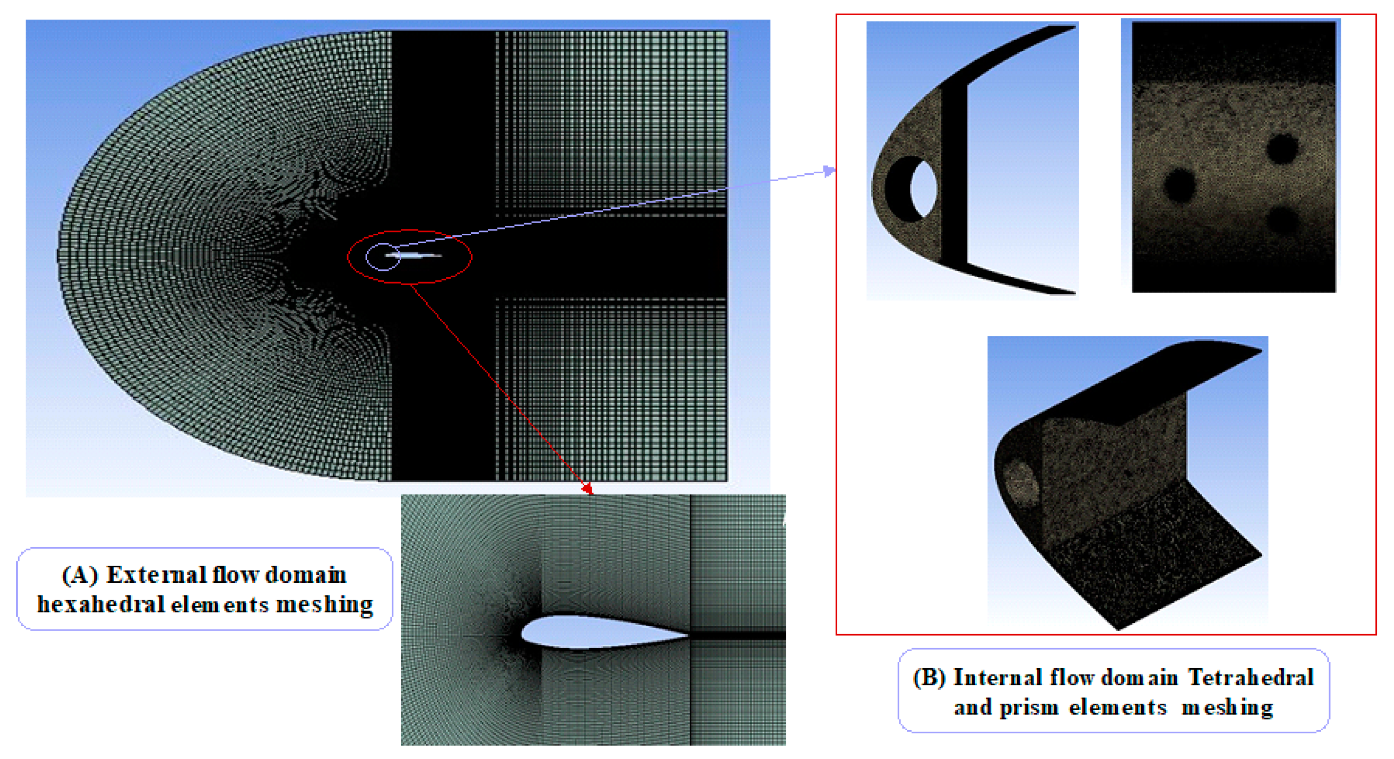
The mesh grid is generated and discretized using ANSYS MESH® 2019 software. To achieve accurate aerodynamic and heat transfer performance on a 3D wing anti-icing system, grids near the 3D wing airfoil section and internal flow domain must be dense enough and the external domain must be large enough to balance calculation time versus the accuracy of the solution. However, extreme fields and grid numbers will consume too many computing resources and slow the speed of the computing process. The hexahedral element is used for the mesh of the external flow domain to minimize the computation time of the solution and the mixed tetrahedral and prism mesh are used for the internal flow domain to get accurate results. For the external flow domain, the multi-block structured grid method is utilized to increase grids near the wing airfoil section using the sizing method, as shown in Figure 6A. In addition, in the internal flow domain, an unstructured multi-block grid type is used to increase the grids near hot air jets by creating a sphere around each jet and using body inflation (see Figure 6B). The method of body sizing is applied to adjust the grid to a small size for the boundary layers of the internal flow domain hot air jets and to increase the size of the grid far from the boundary at a precise growth rate. The domain meshing has an average Skewness of about 0.186035. As a result, it is considered a high-quality mesh. Finally, the total cell number of the full model is about 2,666,876 cells.

3. Internet of Things (IoT)

The IoT is defined as a collective network that combines connected devices and different types of technology, which in turn, facilitates communication between the cloud and these devices [38,39,40]. Due to the emergence of cheap microchips for computers as well as high-bandwidth communication systems, the world now has many devices connected to the Internet that have different functions and tasks [38,39,40,41].
This means that most devices and equipment can exploit sensors to collect data and benefit from them in allowing the design and use of AI to help with ease of use and improve the performance of these systems with the addition of many functions [39,40,41,42,43]. One of the most important tasks of an efficient IoT system is to collect and exchange data from sensors in real time. Among the most important components of an IoT system are smart devices, the IoT application program, and a graphical user interface (GUI) [44,45,46]. Smart devices are devices that have computing capabilities. In these devices, data are collected from the environment of the devices, user inputs, or user patterns, and these data are transmitted via the internet to and from the IoT application. Various methods are used to analyze this data, including AI and ML, in order to make correct and distinct decisions [45,46]. After decisions are made, they are sent back to the IoT device, and then the system responds to implement these decisions, relying on smart inputs. A common example is the use of a website or mobile application to record all data, make decisions, and control devices [38,39,40,41,42,43,44,45,46].

3.1. IoT in Aviation

The IoT gives the aviation industry and airlines access to advanced analytics that unlock new opportunities [38,39,40,41,42,43,44,45,46]. Through the application of the IoT, it is possible to know the behavior and condition of aircraft components. As for airlines, they can create extensive advertising campaigns by collecting data on customers’ opinions, requirements, and behaviors [42,43,44,45,46]. In the case of merging AI with the IoT, the data are converted into actions and decisions in aircraft. The data collected from sensors distributed across the aircraft and historical trends can be used to predict the future behavior of the aircraft’s equipment and components. For example, this method can be applied to predicting aircraft maintenance accidents by pairing warranty information with collected IoT data [38,39,40,41,42,43,44].
The application of the IoT also helps in increasing safety, as the continuous monitoring of aircraft parts leads to improved efficiency and reduces potential safety risks that may occur in the aircraft. For example, the data collected from the plane’s de-icing system can be used to predict potential disasters as a result of the risks caused by ice on the aircraft. It is also possible to record problems that constantly occur in the aircraft and then predict their occurrence and find solutions to these problems [40,41,42,43].

3.2. ThingSpeak Platform

In light of the continuous progress and the emergence of Industry 4.0, control and monitoring systems have been designed using sensors that have aroused the interest of many researchers and engineers [39,40,41,42]. In addition, mobile phones and various websites have been used to implement these solutions. Users are able to control and monitor electrical and mechanical services from thousands of kilometers away using IoT technology.
Remote control tools are used via the Internet. ThingSpeak is a platform that acts as a carrier for data packets between host microcontrollers [39]. Through ThingSpeak, users can choose the method of controlling the connection and whether it is private or public. Therefore, in recent times, it has become one of the most popular methods for collecting information from sensors and realizing the IoT. ThingSpeak has an open API on the Internet that allows users to create channels to monitor and send information [39,40,41,42]. It is open-source software written in Ruby that allows users to control and monitor Internet-enabled devices. It also facilitates the recording and dissemination of data by providing an API for each of the social networking sites and devices used [41]. It was designed in 2010 by ioBridge as a tool to assist IoT applications and has since been integrated with Matlab. It is considered an important tool that allows researchers to develop prototypes to analyze and visualize data and send important alerts to IoT systems without the need to develop web programs or set up servers [42].

4. Artificial Neural Network (ANN)

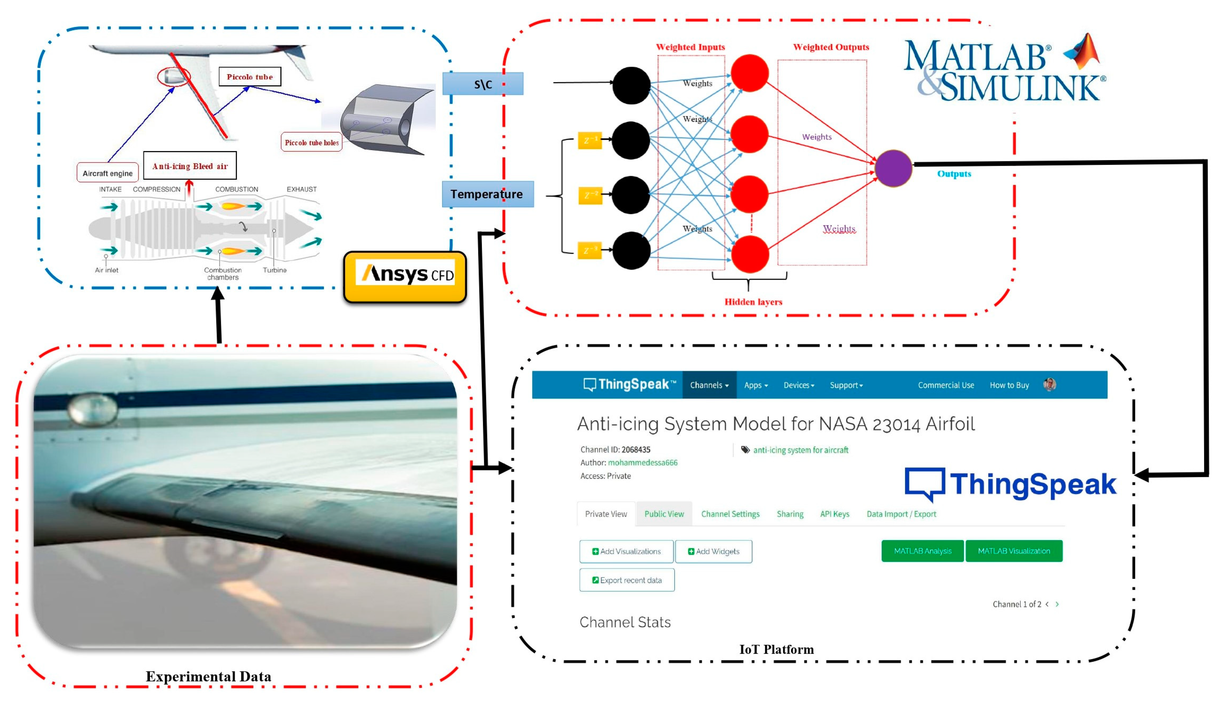
ANNs are considered a subset of ML [25,26,27,28,29,30,31,32,33,34,35,36,37]. ANNs are considered one of the most important elements of deep learning, as they lie at the heart of the algorithms underlying this learning. In terms of their structure and components, ANNs are similar to the human brain [28,29,30,31,32,33,34] and mimic the way that biological neurons work with each other. One of the most important components of an ANN is the node. Each ANN consists of a set of node layers. The layers consist of an input layer, a number of hidden layers, and an output layer. Each node, or artificial neuron, connects to another and has an associated weight and threshold. If the output of any individual node is higher than the specified value of the threshold, that node is exited and activated, and data are sent to the next network layer [25,26,27,28,29,30,31,32,33,34,35,36,37]. Otherwise, no data will be sent to the next network layer. Neural networks depend on training data to learn and improve their accuracy over time, which will effectively affect the efficiency of this structure. However, once the learning algorithm has been fine-tuned, ANNs become one of the most powerful tools in artificial intelligence and computer science, allowing users to classify and aggregate data at high speed [25,26,27,28,29,30,31,32,33,34]. For example, an image or speech recognition task can be completed in minutes using ANNs compared to hours using manual recognition by human experts. Therefore, neural networks have been applied in many applications, such as the Google search algorithm—the most famous example—weather prediction, and the classification and control of aircraft malfunctions [25,26,27,28,29,30,31,32,33,34,35,36,37]. The structure of the proposed data transfer in the wing anti-icing system is given in Figure 7. In this article, the data are organized based on the availability of data. The data consist mainly of experimental data taken directly from anti-icing system measurements. The time needed to implement a typical ANN inference or operation may change depending on the complexity and size of the network and the hardware required for computation. Overall, simpler and smaller ANNs can be executed in a matter of microseconds or milliseconds, while complex and larger ANNs can require several seconds or minutes to finish a single inference [25,26,27,28,29,30,31,32,33,34,35,36,37]. In this paper, the time required for the trained ANN to make an inference is of the order of minutes.
The performance of the proposed forecasting network structure is evaluated based on the following metrics: mean square error (MSE), max relative error (MAE), and absolute variance ( R 2 ) (Equations (1)–(3)). The m stands for experimental or CFD data. If the CFD data are used, T m = T C F D , T m m a x = T C F D m a x and T m m i n = T C F D m i n . The same concept applies to the experimental data. These criteria are considered acceptable tests for the behavior of ANNs. In addition, R 2 = 1 means an excellent fit and an R 2 of near 1 means a good fit. As a result, there is a proportional relation between the values of R 2 and the quality of the fit.
M A E   % = M a x   ( T A N N T m T m m a x T m m i n ) × 100
M S E   % = 1 n i = 1 n T A N N T m 2 T m m a x T m m i n × 100
R 2 = 1 i = 1 n T A N N T m 2 i = 1 n T A N N T A N N m e a n 2
where: n is the number of samples, T A N N is the temperature predicted by the neural network, T m is the actual measured or CFD-calculated temperature, T m m a x , T m m i n are the maximum and minimum measured or CFD-calculated temperature, respectively, and T A N N m e a n refers to the mean value of the temperature predicted by the ANN.

5. Results and Discussion

The discussion is divided into three scenarios based on the methodology used. The three scenarios are based on a numerical analysis based on CFD, predictions provided by ANNs, and the use of ANNs with an IoT platform.

5.1. Scenario 1: Numerical Analysis Based on CFD

5.1.1. Grid Dependency Check

To decrease the number of grid elements without compromising accuracy, a grid independence check was performed. In general, utilizing more cells makes a numerical answer more precise, but doing so also increases the amount of computer memory and processing time needed. To inspect the independence of the results versus cell number, nine kinds of meshes were investigated (Table 2). Grid one has about 166,140, 12,348, and 164,319 elements for the external domain, solid domain, and internal domain, respectively. While grid nine has about 685,250, 28,560, and 1,953,066 elements for the external domain, solid domain, and internal domain, respectively.
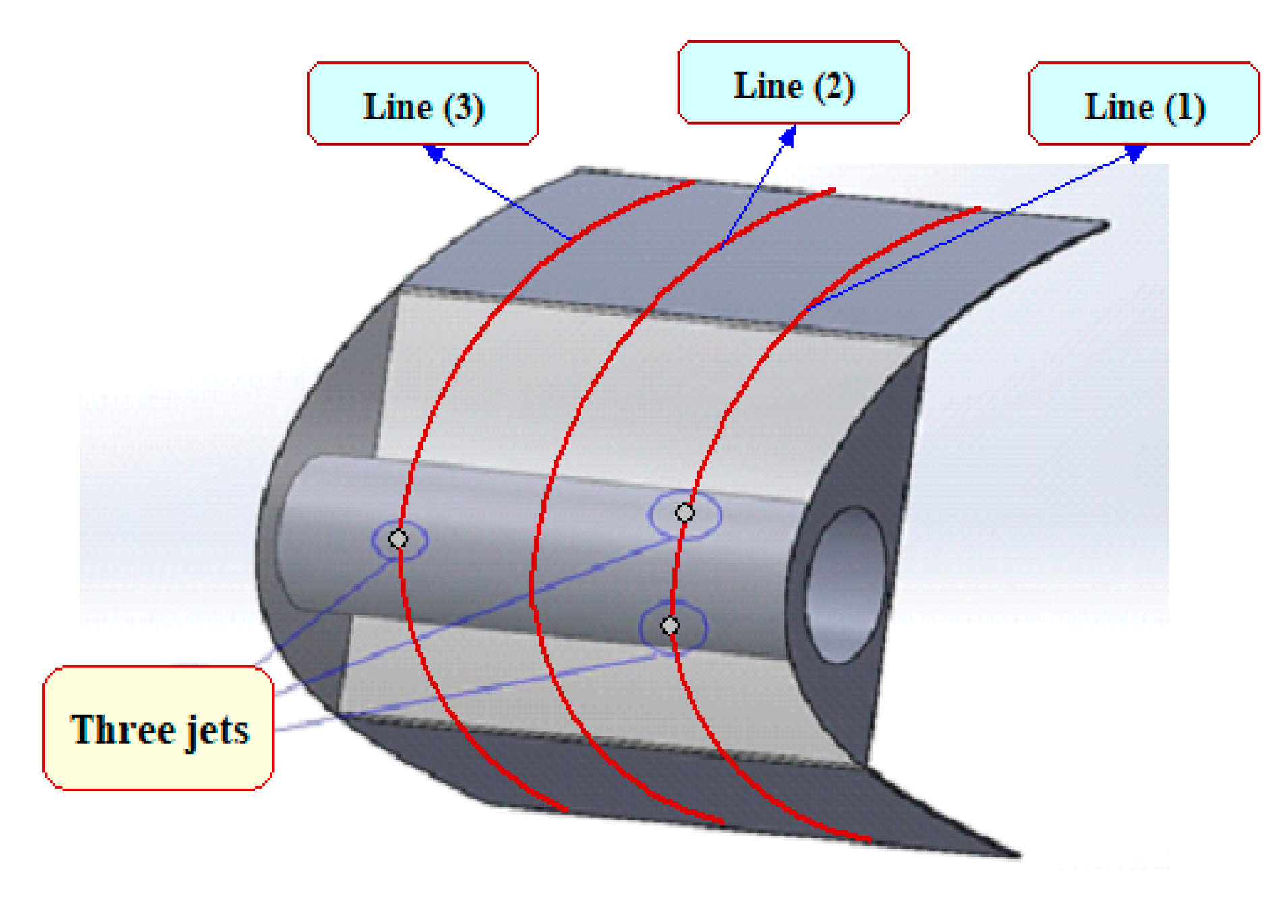
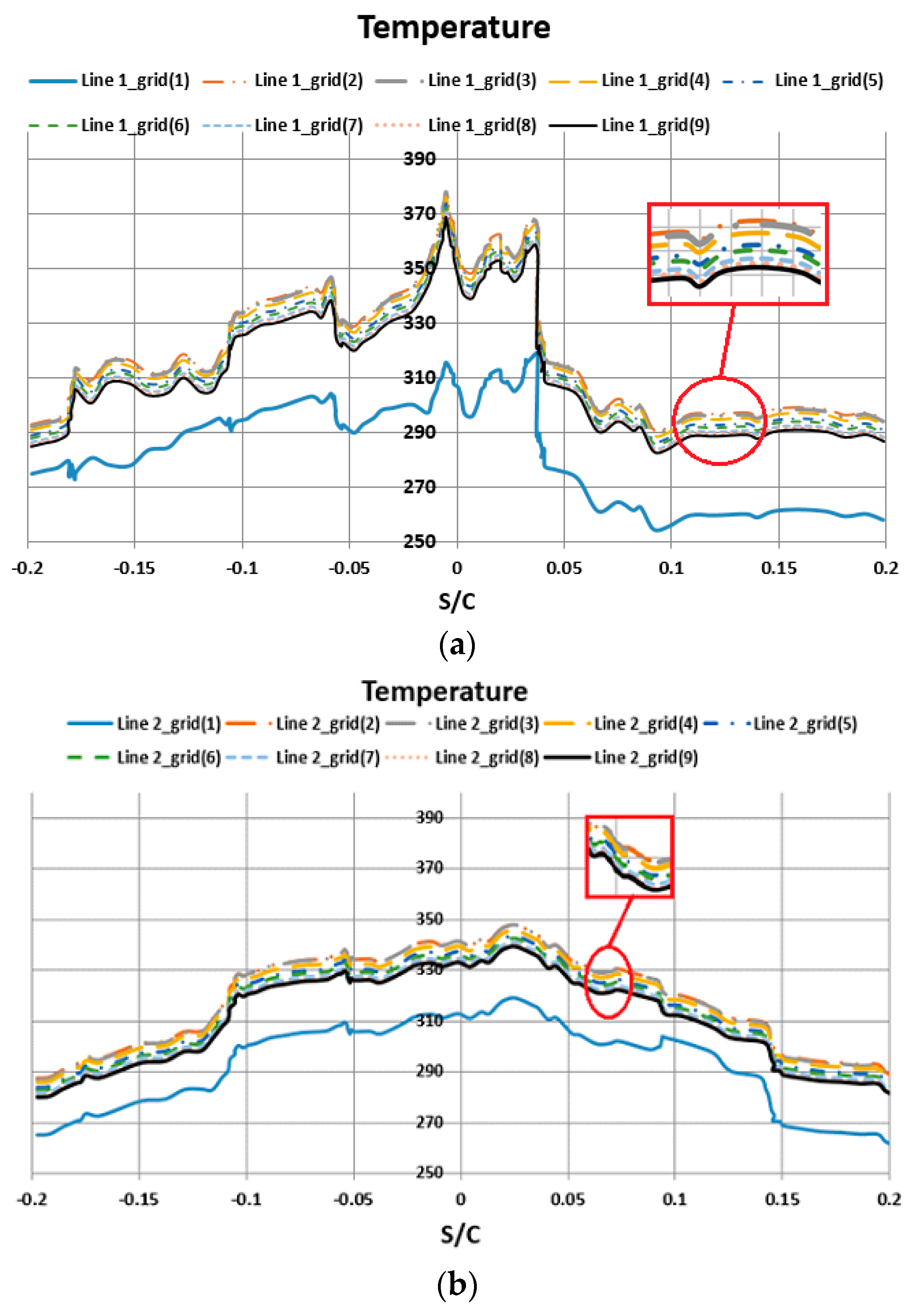
In common with [23], in this study, the shape of the ice on the NACA 23014 airfoil is modeled using LEWICE 2019 software. In the experimental procedure, thermocouples are used to measure temperature along three lines on the wing leading edge surface. The points of line 1 are set over the centerline of hot air jets 2 and 3, while, the points of line 3 are set over the centerline of hot air jet 1, and the points of line 2 are set at the span location between the hot air jets, as shown in Figure 8. The thermocouple used is a composite of iron and copper-nickel materials. It consists of a brass tip, 1/4 thread adapter (BSP), 19 mm diameter aluminum bayonet, 2 × 24 metallic braid cable, and pin or fork connection terminals. The measuring range of the thermocouple is −40 to 750 C. The average thermoelectric power is about 5.65 mV/100 C. The produced electromotive force is about 0 to 42,922 mV. Figure 9a–c show the effect of the number of grid cells on the temperature in (K) measured along the three lines of the wing anti-icing system. After the seventh grid, it is very clear that the results are almost unaffected by increasing the number of grid cells. Thus, eight grids can be used to maintain accuracy while reducing the time of solution. All these calculations were carried out by using the ANSYS CFX® 19 solver and a computer with an Intel Core i7 and 16 GB RAM, and the criterion of convergence was set to decrease the scaled residual below the value of 10−6.

5.1.2. Verification of Numerical Model

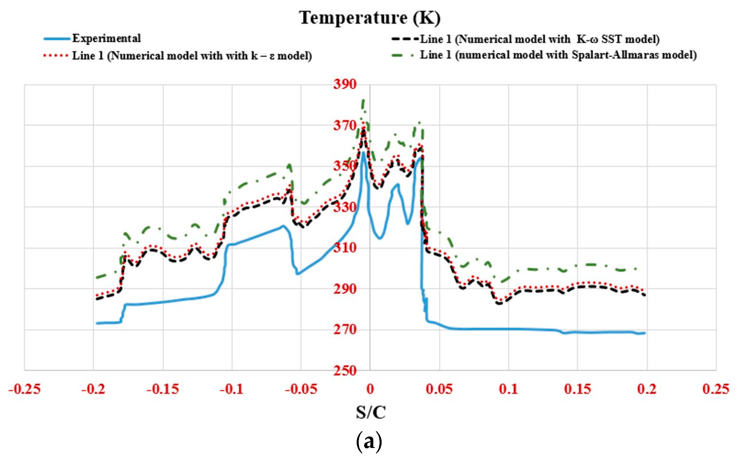
The grid size and type are developed to verify the numerical model with the experiment results based on the same boundary conditions reported in [23]. The experimental data are obtained from [23]. Figure 10 shows the comparison between the obtained numerical results with various turbulence models (k–ε, k–ω SST, and Spalart–Allmaras) and experimental measurements for temperature distribution on the three-line surface distance per chord (S/C). The surface distance per chord (S/C) is measured from the reference point on the wing leading edge. Negative (S/C) values are described for the lower surface and positive for the upper surface. It can be seen that the temperature is high in surface nodes opposite to inlet jets and decreases gradually on other surface nodes. A good agreement between the numerical and experimental results is demonstrated for the three lines of thermocouples. The k–ω SST turbulence model provides numerical results closer to the experimental measurements than those of the other turbulence models along all three lines, as shown in Figure 10a–c. The average percentage error of the numerical results with the k–ω SST turbulence model compared to experimental measurements for lines 1, 2, and 3 is 5.62%, 4.23%, and 5.36%, respectively. The use of the k–ω SST turbulence model for anti-icing models is recommended in many studies [23,50,51,52].
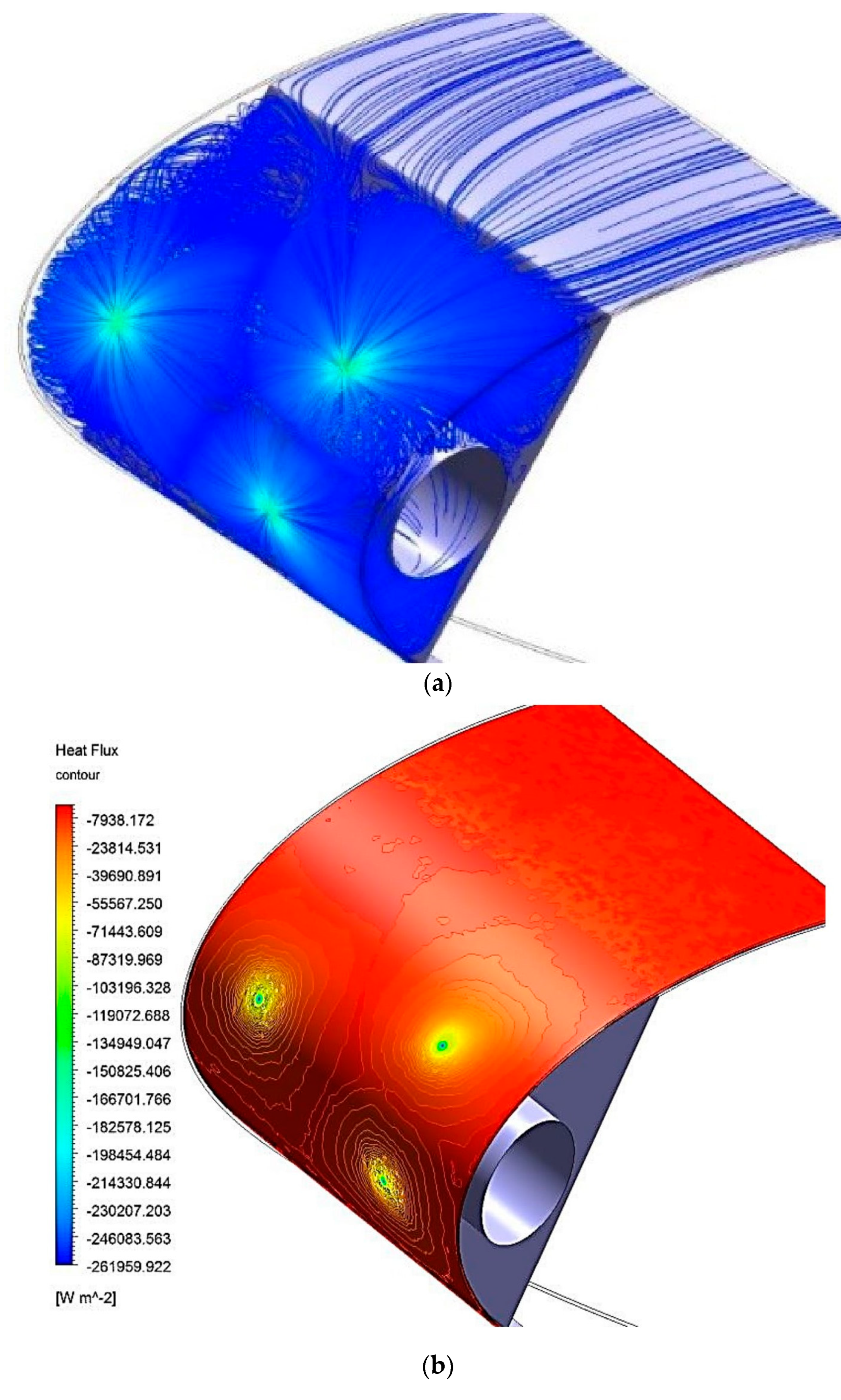
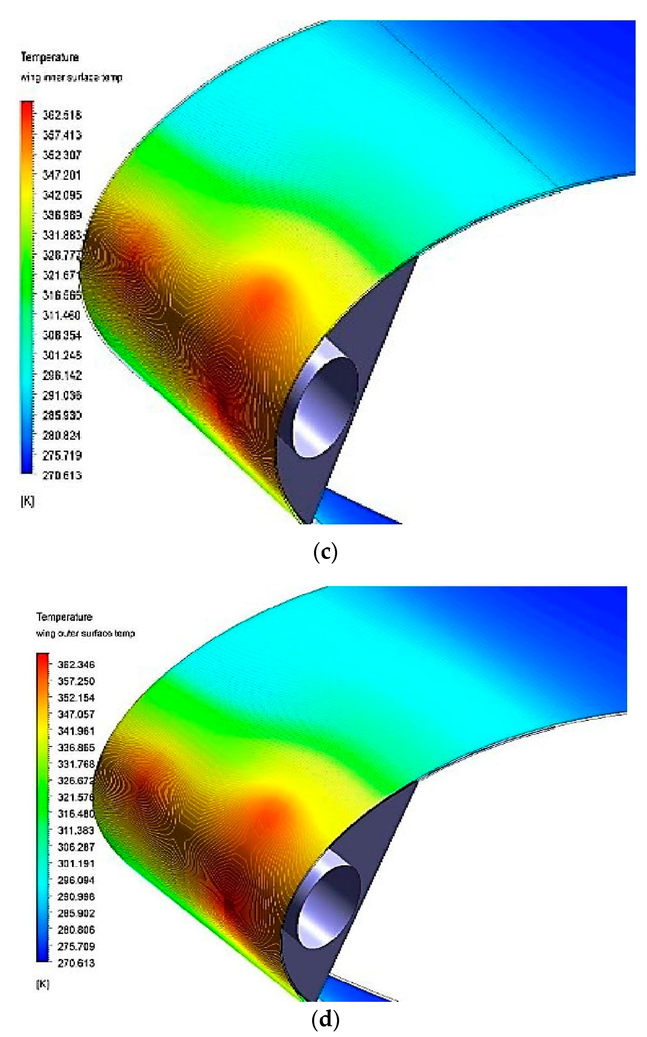
The streamlines of the internal flow domain are investigated in this study. Hot air is ejected from the tube through three jets and fills the leading edge area with large eddies and vortices. The stagnation points of three of the hot air jets are illustrated in Figure 11a. From Figure 11b, the contours of the heat flux in W/m2 are illustrated over the wing’s outer surface. There is a high heat flux in the area opposite the jet outlets, which reduces gradually across the surface. Figure 11c,d illustrate the temperature contours (K) on the leading edge outer and inner surfaces. There is a high temperature in the area opposite the jet outlets, which reduces gradually across the surface.
It is apparent that the temperature on the outer surface was lower than the temperature on the inner surface due to conduction losses in the solid wing.
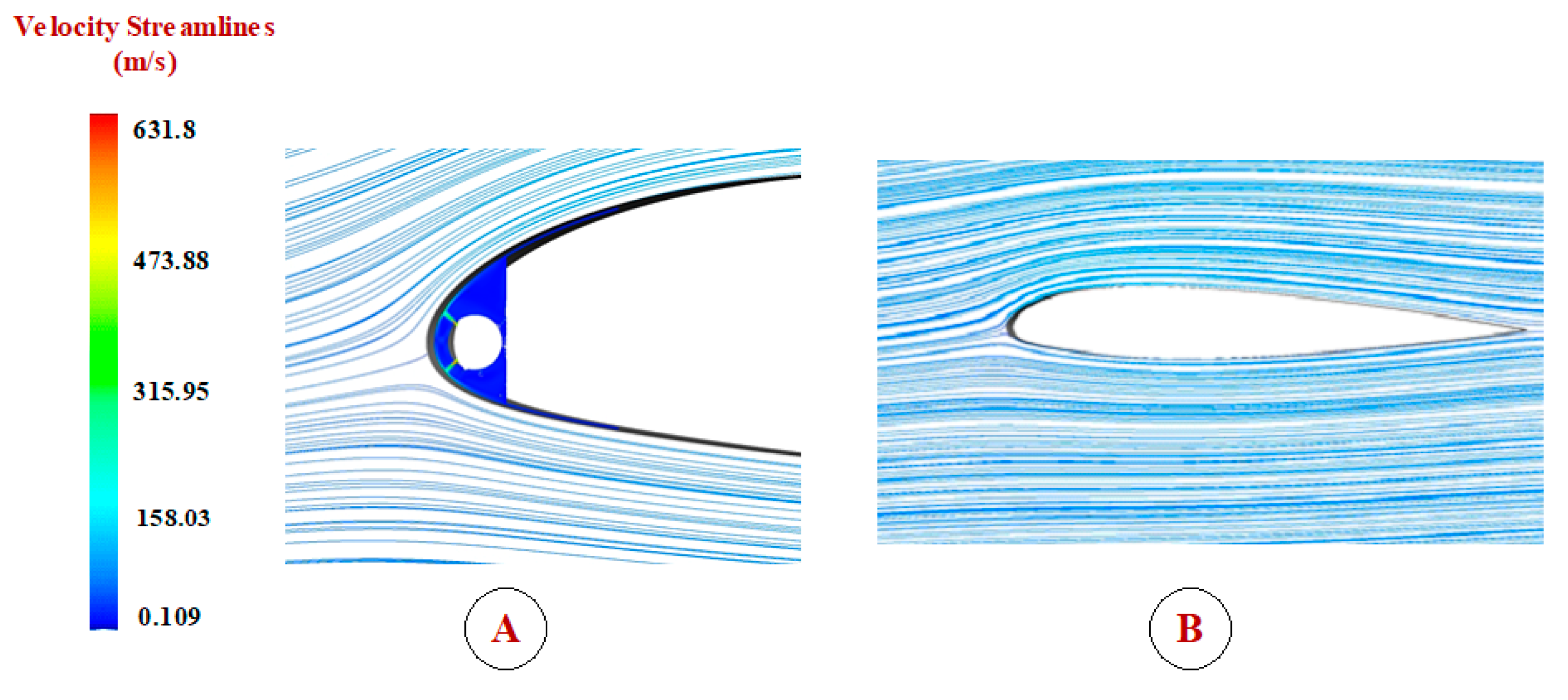
The shape of the velocity streamlines of the internal and external coupled flow domains was also investigated. Figure 12A illustrates the shape of the velocity streamlines of the internal flow domain.
The hot air is ejected from jets and it fills the leading edge area with large eddies and vortices. Figure 12B illustrates the shape of the velocity streamlines of the external flow domain. The cooled air flows smoothly along the airfoil configuration with an angle of attack of 3 degrees.
The velocity contours of the internal and external coupled flow domains are obtained (see Figure 13A). In addition, the velocity values of the external domain with zero value at the stagnation point are obtained at an angle of attack of 3 degrees, representing cooled air impinging on the external solid surface. Figure 13B shows an expanded section of the velocity contours around the internal flow domain. The velocity values of the internal domain, with maximum values at the hot air jets, are demonstrated, representing hot air impinging on the internal solid surface.
The shape of temperature contours of the internal and external coupled flow domains are illustrated in Figure 14. A modular method that split the physical domain into three domains was used to explain the hot-air anti-icing challenge (internal, external, and solid domain). Intended for the internal domain, the hot air is ejected from holes in the piccolo tube for forced convection heat transfer between the internal flow domain and the internal surface of the solid domain. In the case of the external domain, the cooled air flows around the airfoil surface for forced convection heat transfer between the external flow domain and the external surface of the solid domain. The solid domain conducts heat from the internal surface of the leading edge to the runback flow on the wing’s external surface.

5.2. Scenario 2: ANN Model Based on Experimental and CFD Data

In this article, the use of ANNs is proposed for predicting the temperature of an aircraft wing anti-icing system. The data used for training, validating, and testing is collected from experimental studies and the results of the CFD simulation. We built two different ANNs based on the data. The first is built from experimental data and then compared with the CFD results. The second ANN is built from data from obtained the CFD simulation. The two types are both presented to facilitate the forecasting process based on the available data, as, in many cases, it is very difficult to obtain experimental data on aircraft to build a forecasting model. The ANNs have four temperature inputs and one output (Figure 15). The inputs are delayed by one sample, two samples, and three samples. The performance of the obtained ANNs is compared based on mean square error (MSE). In addition, the Levenberg–Marquardt method is adopted for training the ANNs.
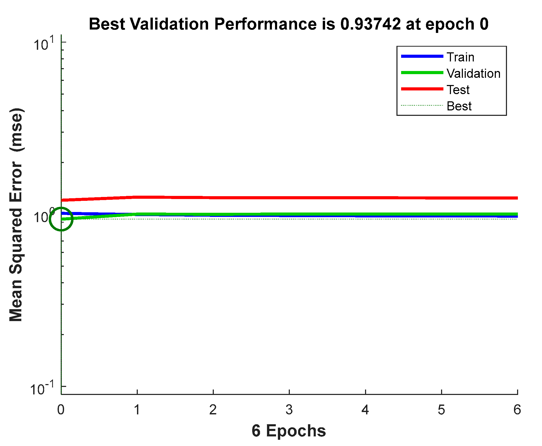
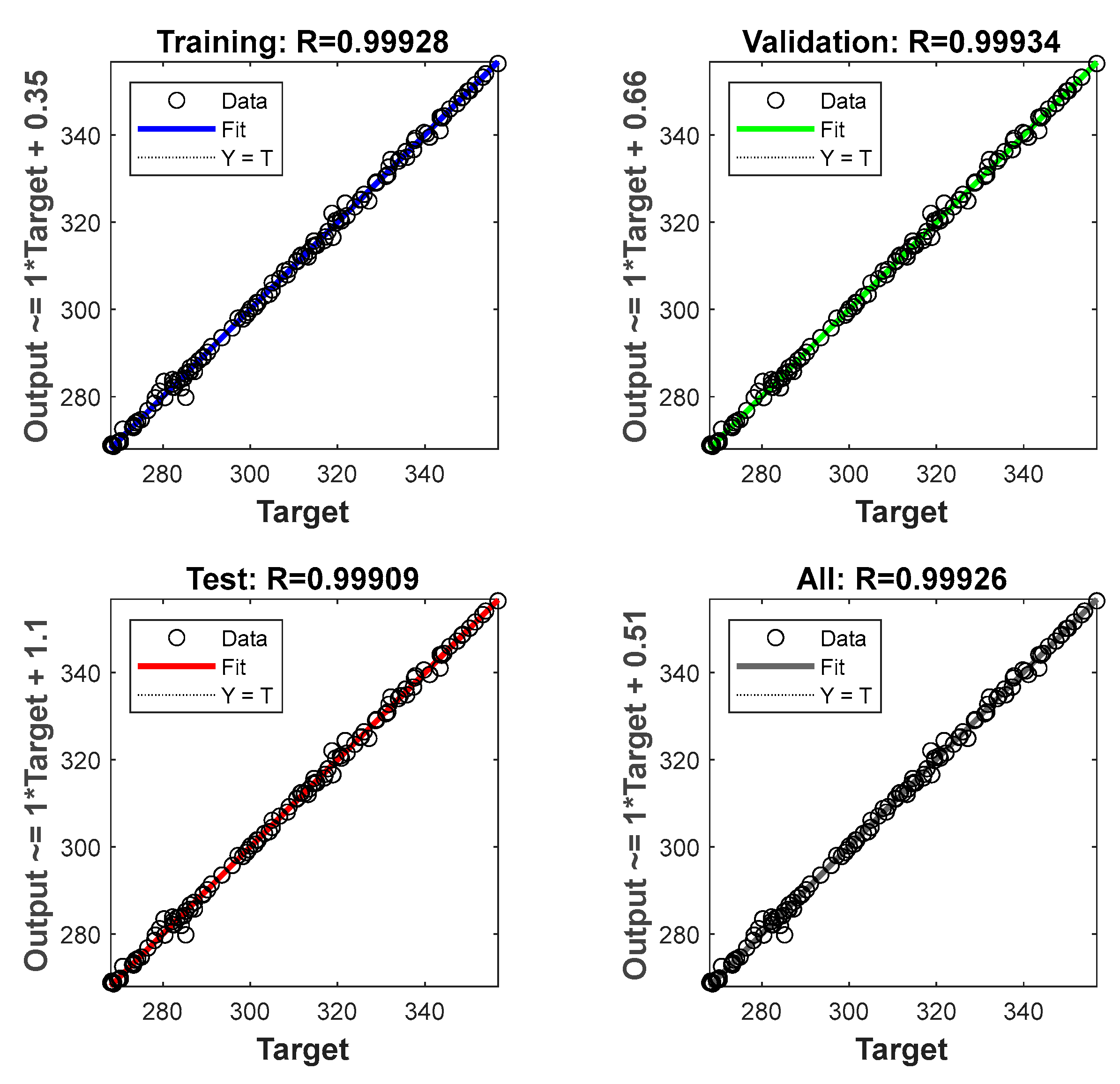
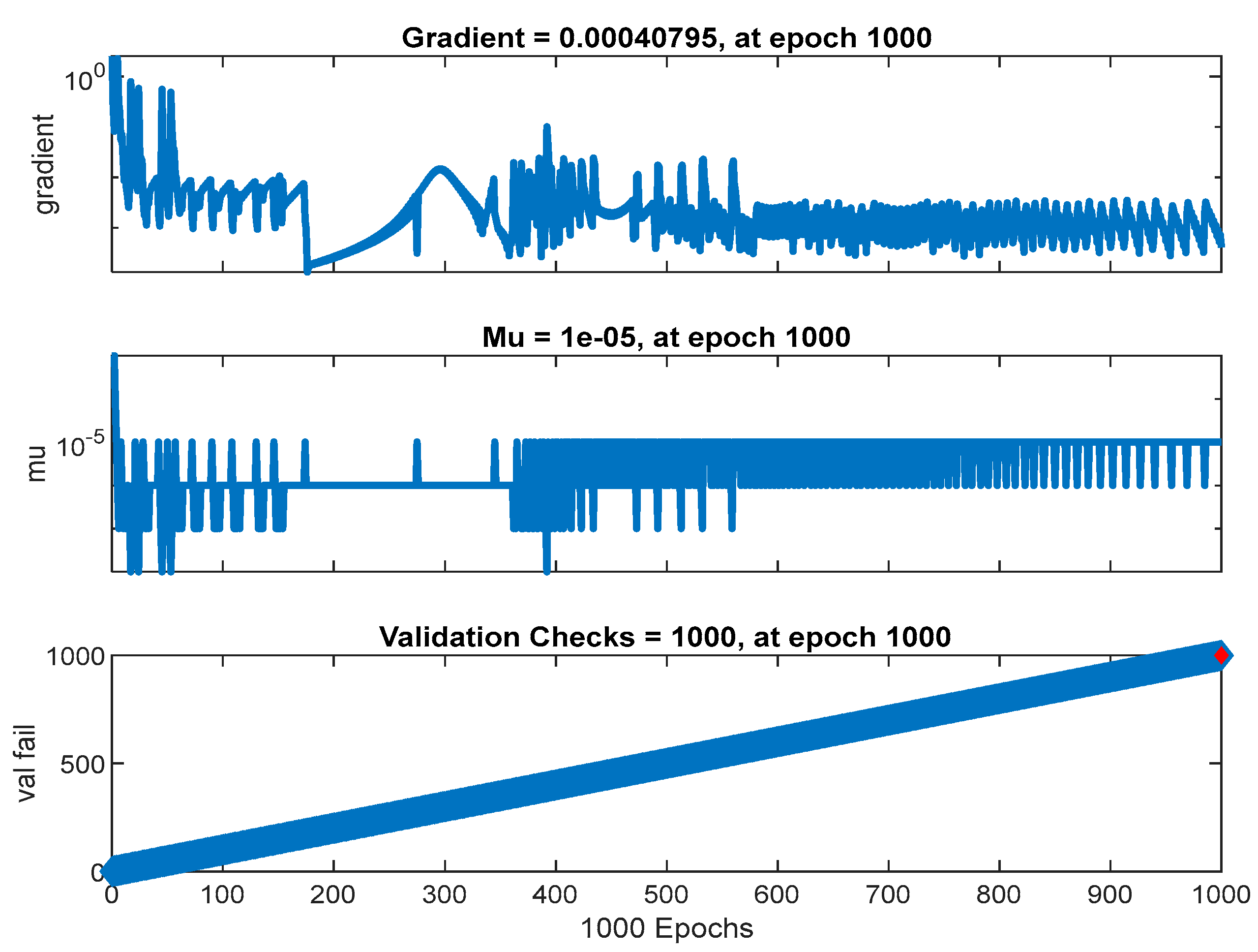
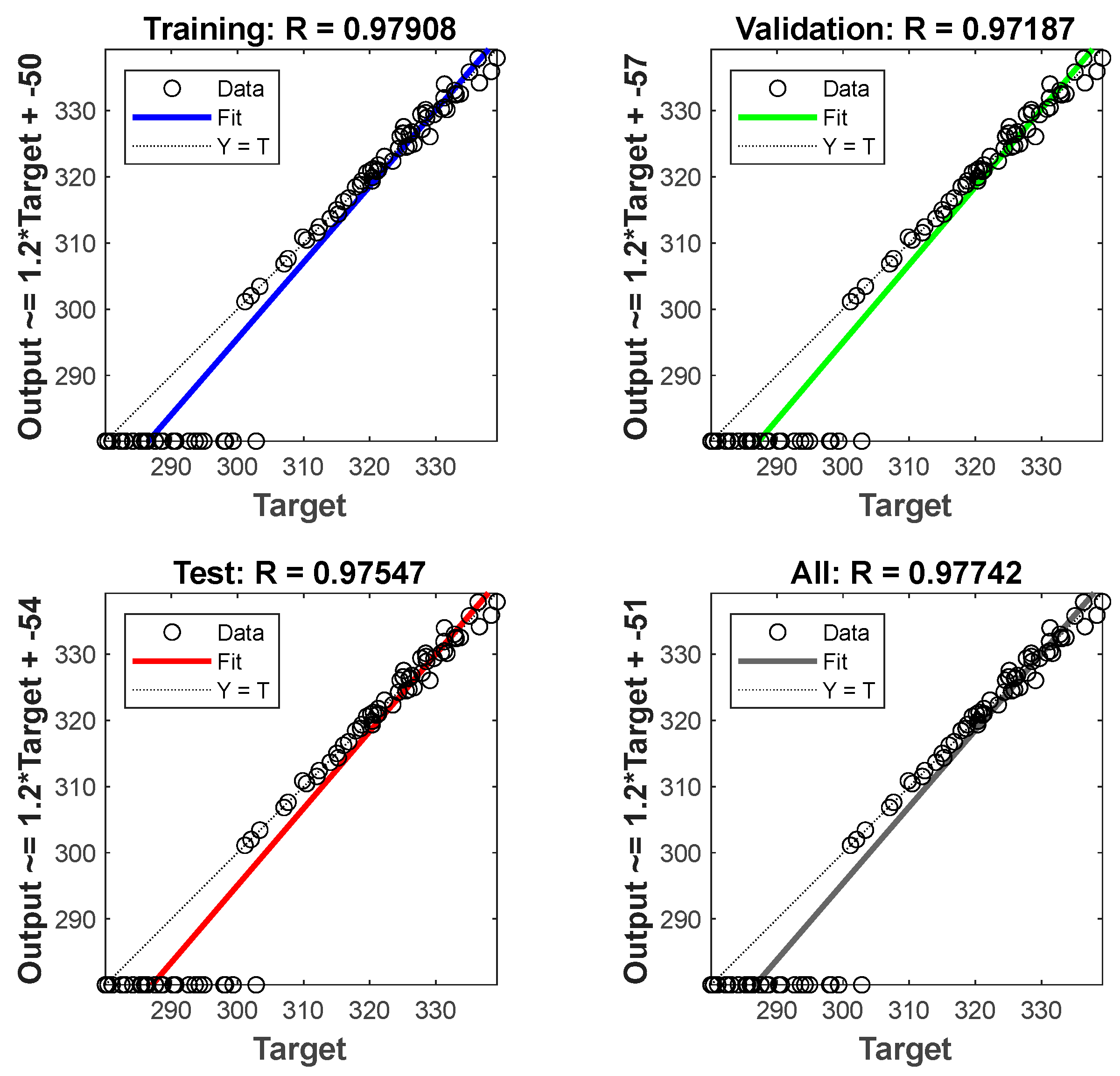
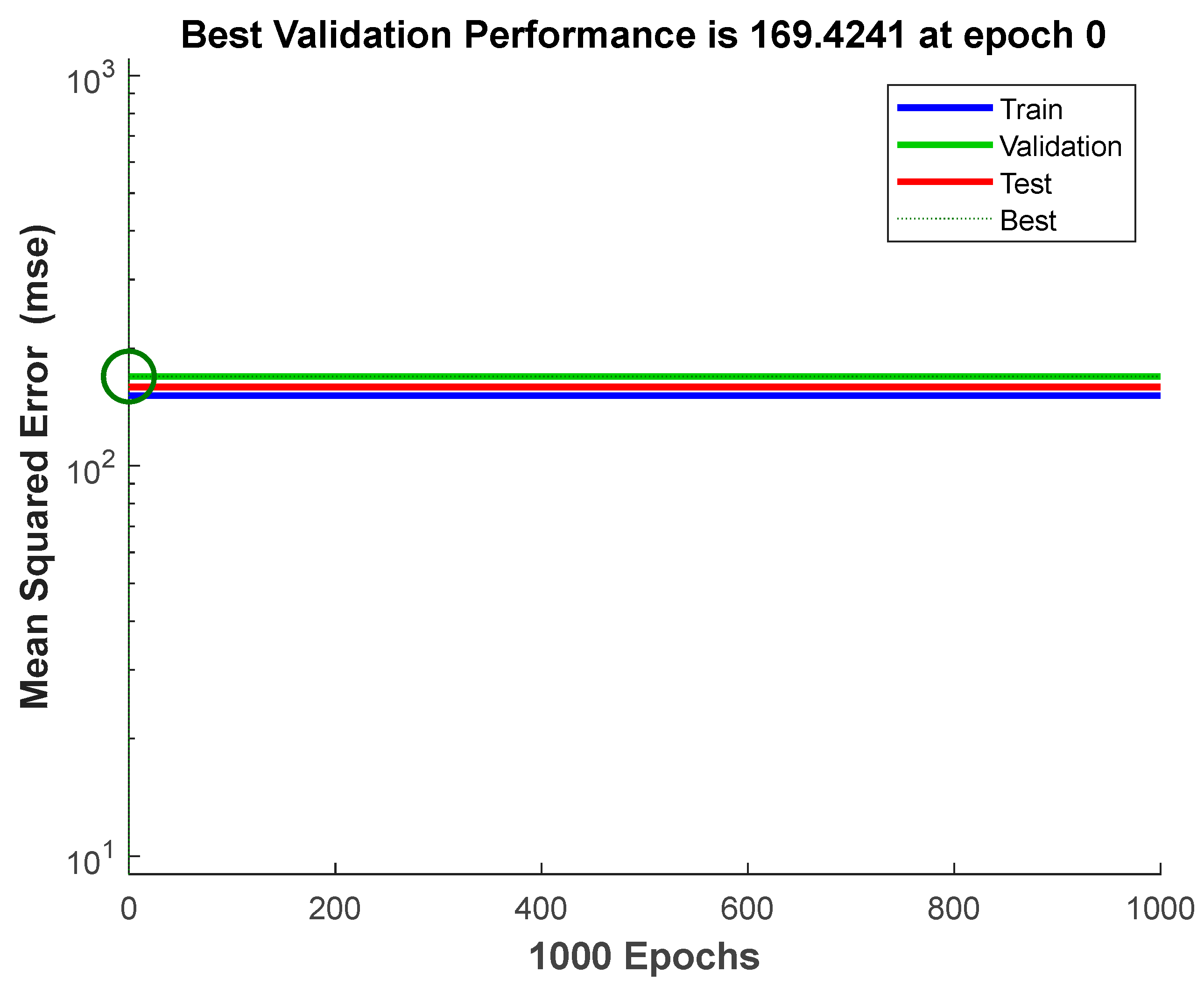
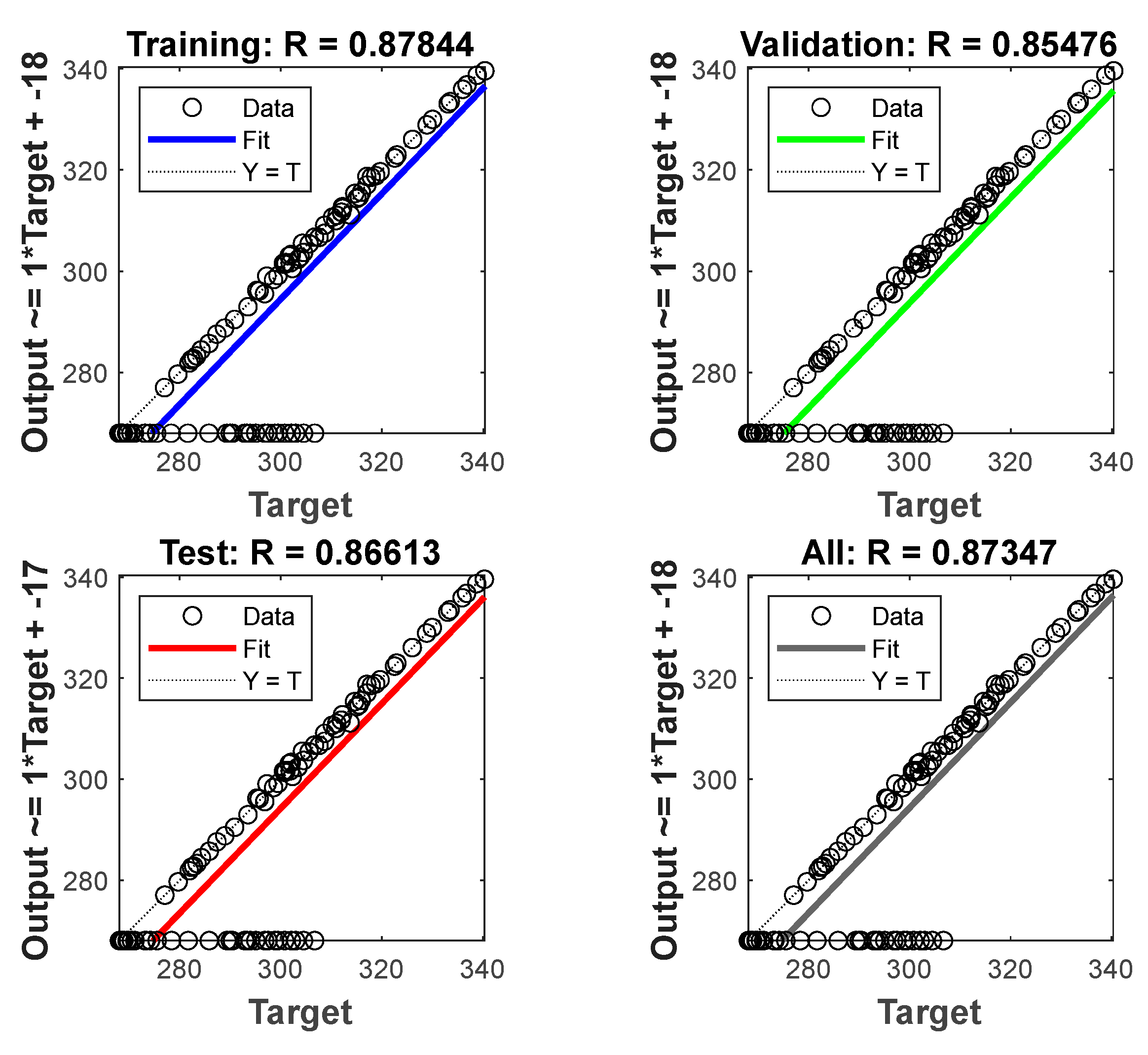
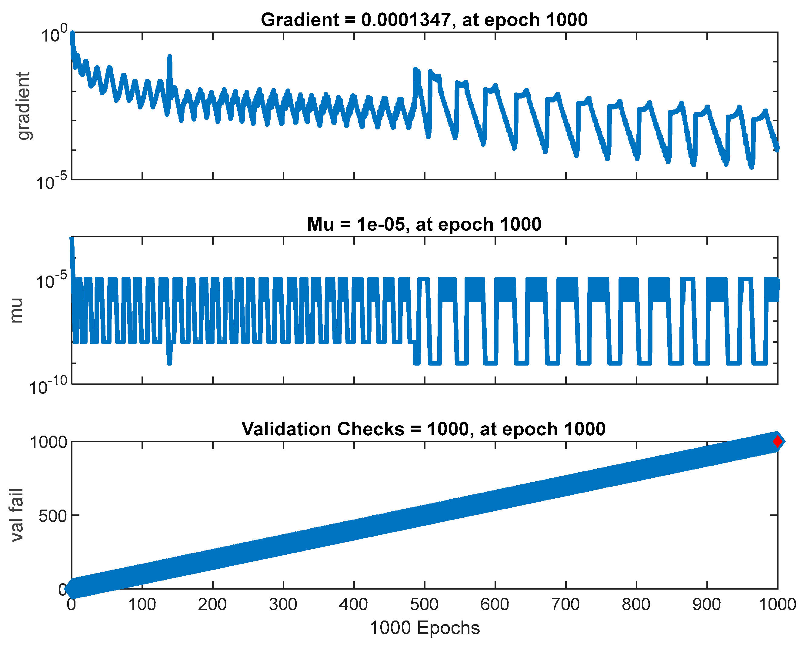
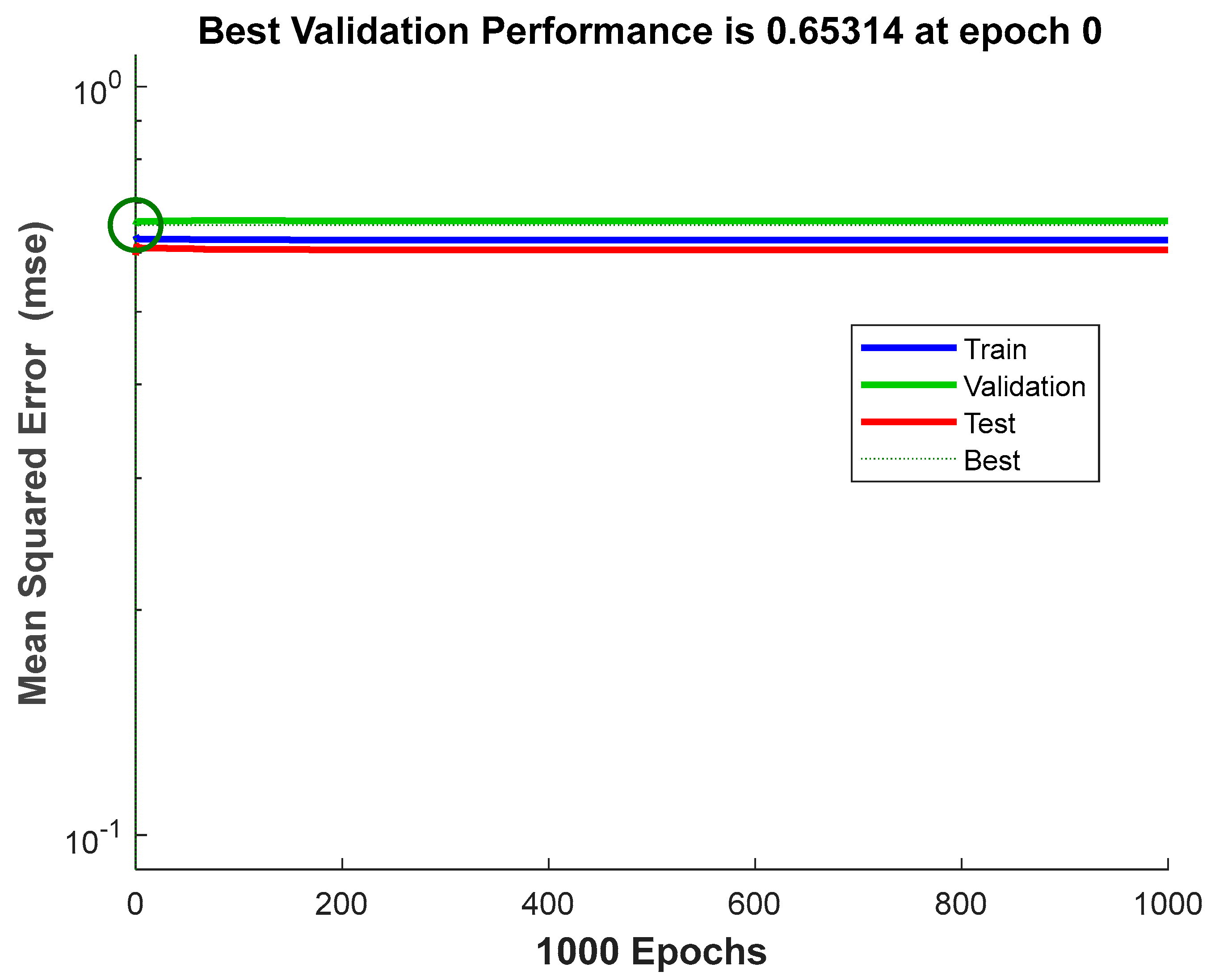
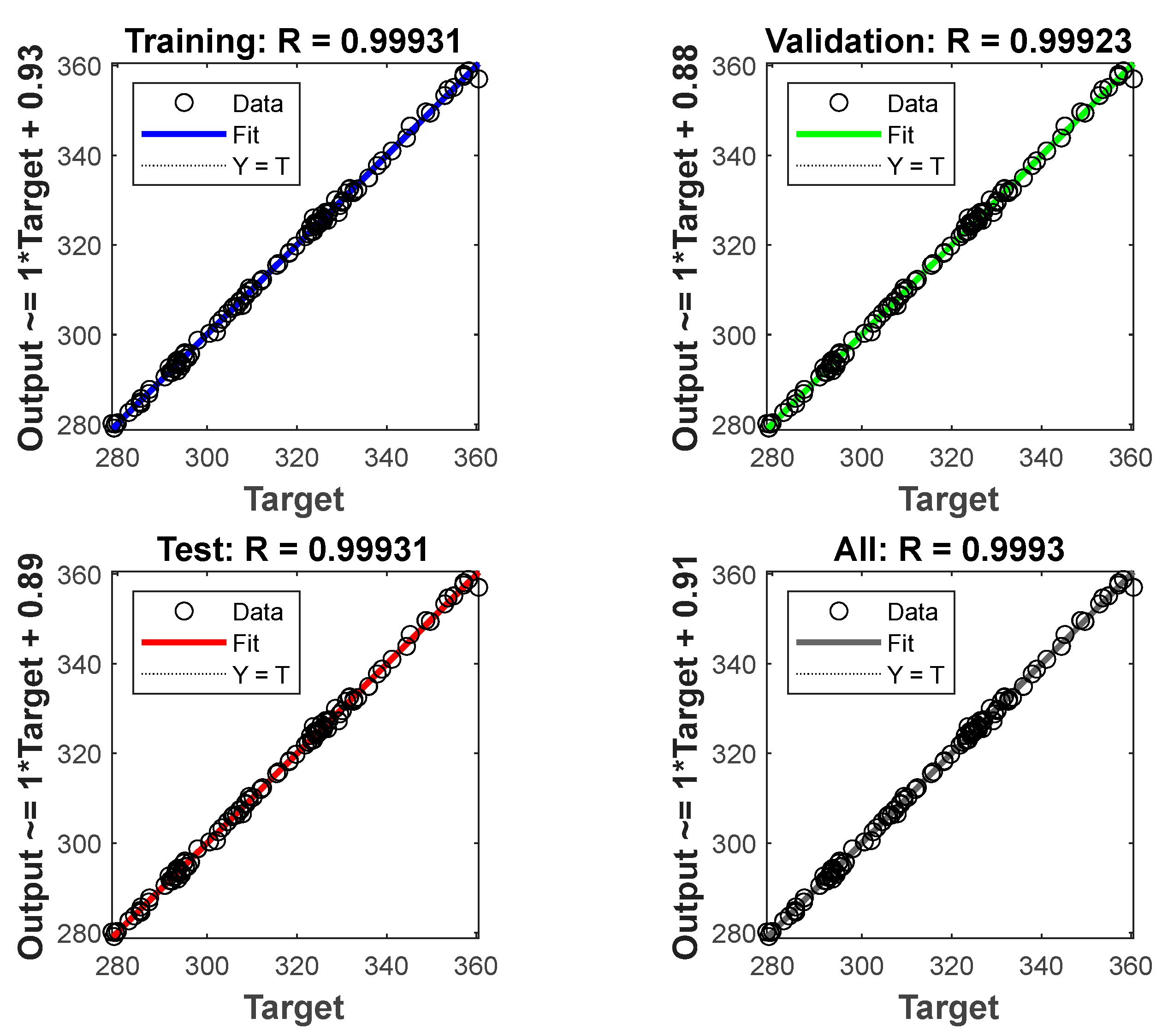
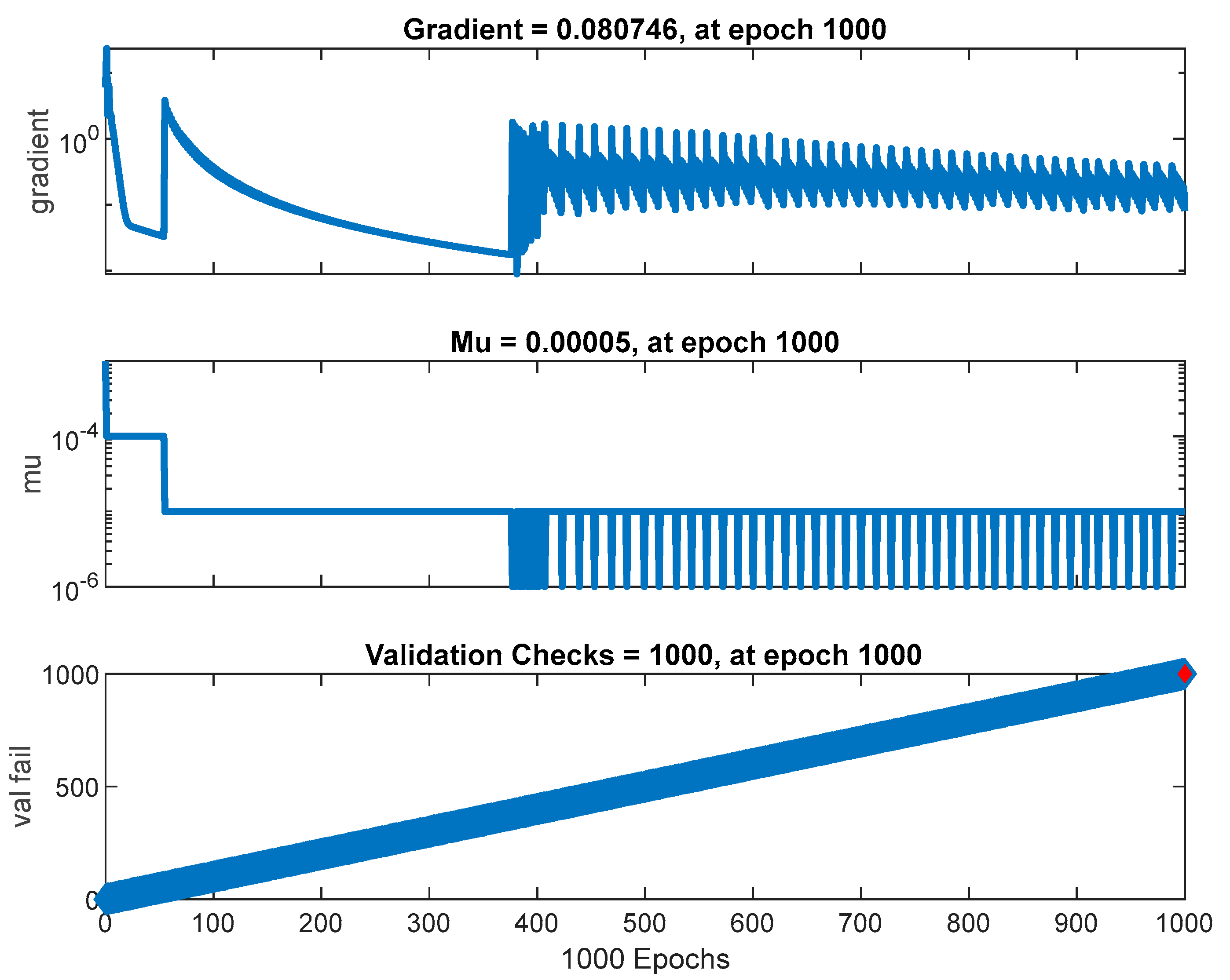
The data used for building ANNs are divided into three categories: training (70%), validation (15%), and testing (15%), with samples from 2019, 2021, and 2017 utilized for lines 1, 2, and 3, respectively (Table 3). The experimental data are used to build an ANN for line 1, as given in Table 3 and Figure 16, Figure 17 and Figure 18. Figure 16 demonstrates the performance of the ANN based on experimental data, which shows a decreasing error with increasing epochs. While Figure 17 demonstrates the good regression performance with values of about 0.99 for training, testing, and validation, In Figure 18, the states of training have been shown for the obtained ANN for line 1. The ANN based on CFD data for line 1 is shown in Figure 19, Figure 20 and Figure 21. Figure 19 shows the training performance for line 1 based on CFD data. It demonstrates the decreasing MSE with an increasing number of trials. Figure 20 presents the regression performance of the ANN based on CFD data for line 1. The regression for training, testing, and validation is 0.99, which means this is an accurate model for predicting the temperature in an aircraft wing. Figure 21 shows a good performance for ANNs for line 1. An epoch is defined as the ANN training with all the training data for one cycle.
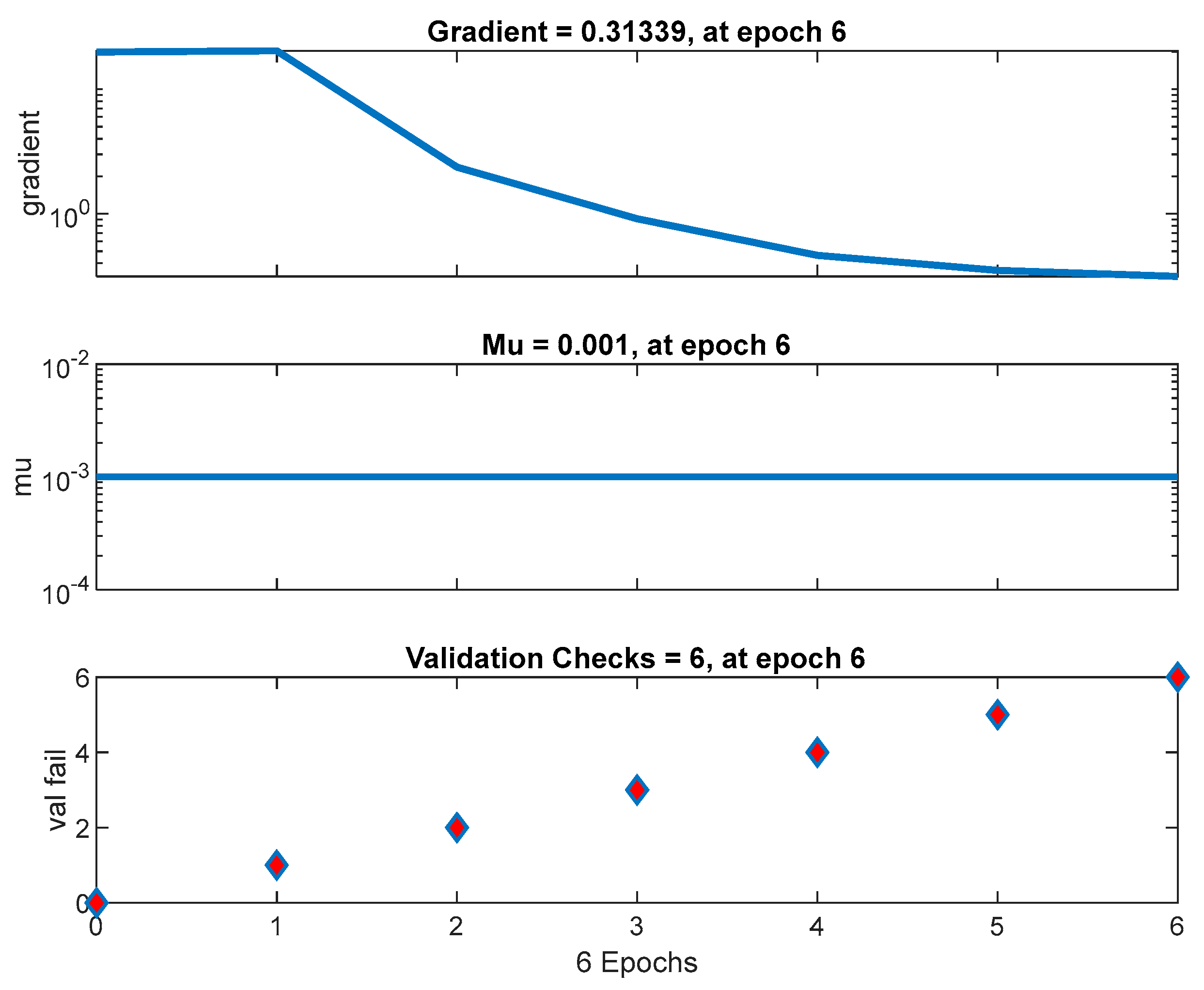
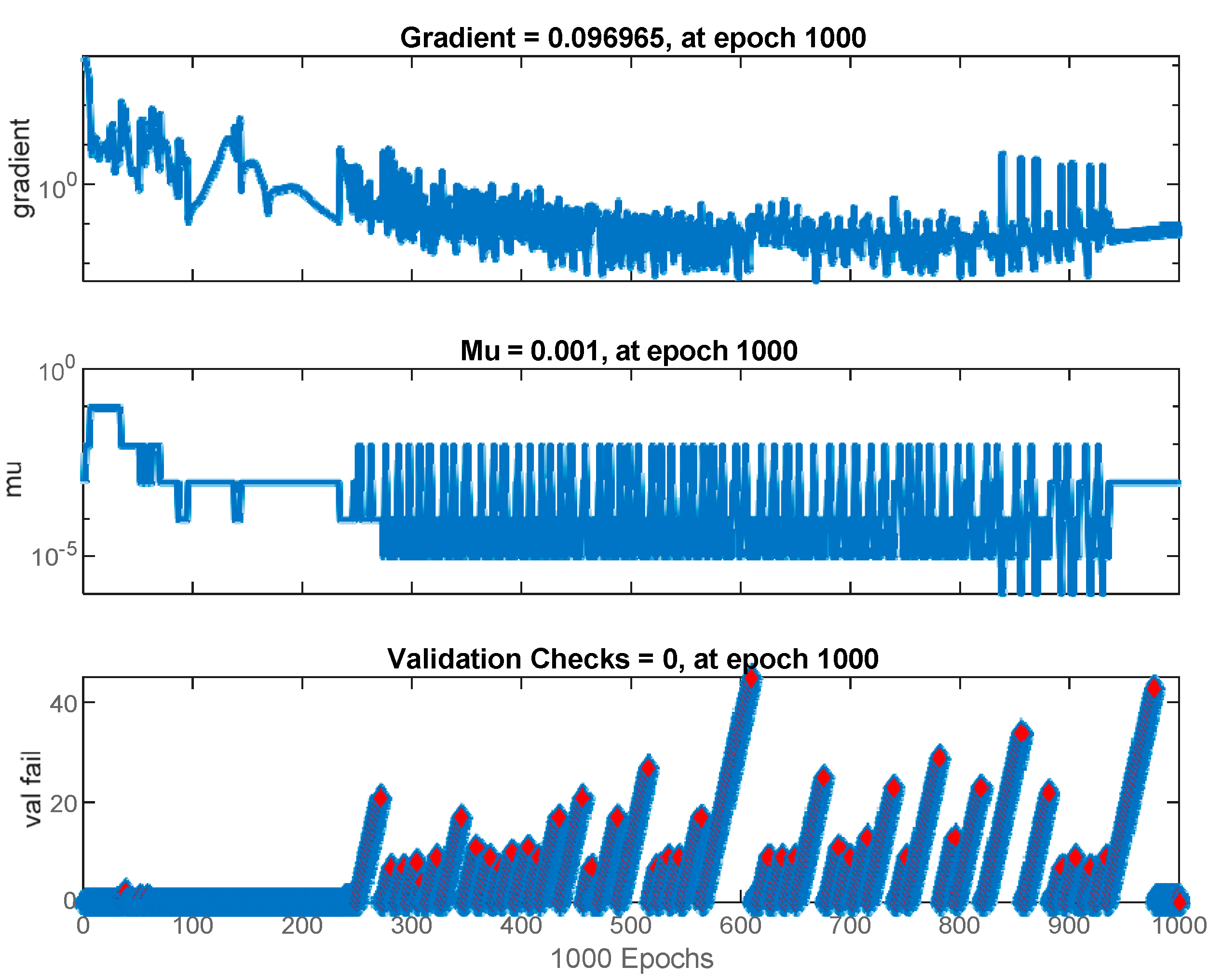
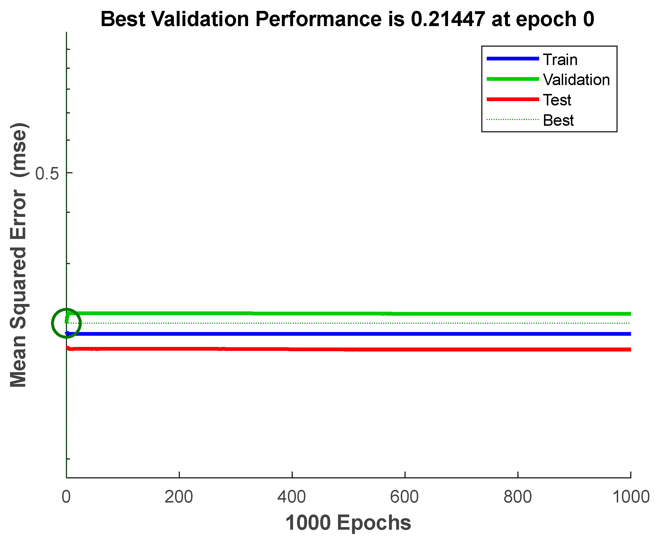
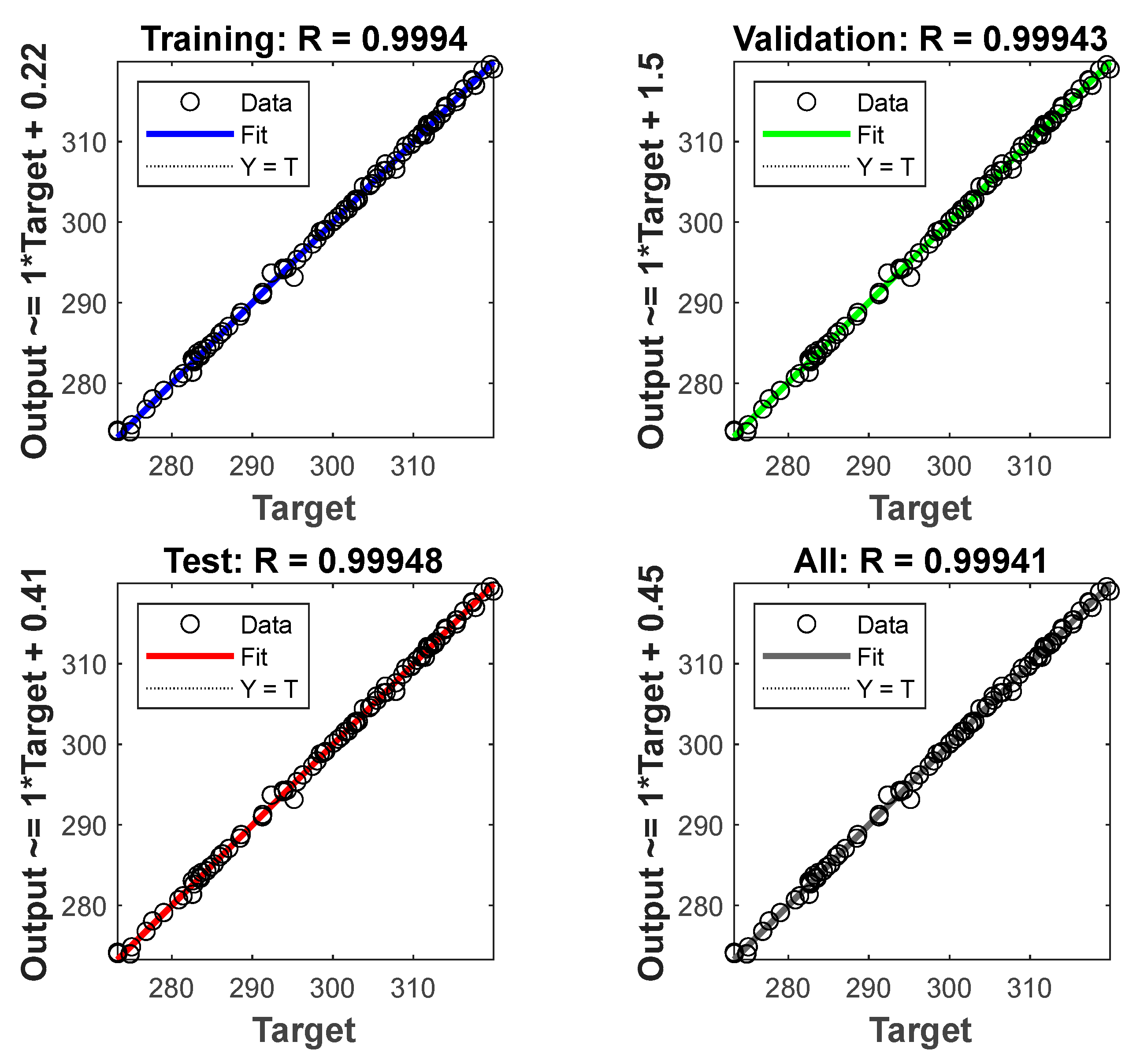
The measured best validation performance is about 0.21447 at epoch 0 for the obtained ANN based on experimental data for line 2. The performance of the training process for line 2 is depicted in Figure 22. In this figure, the MSE is less than 0.5, which indicates a good ANN model. Moreover, the evaluation of training, testing, and validation is around 0.999 for training regression, as given in Figure 23. The training state performance for line 2 is shown in Figure 24. The obtained CFD data were also used to build an ANN for line 2. The performance of the ANN is presented in Figure 25, Figure 26 and Figure 27. These figures indicate an acceptable performance for the obtained model for line 2. The performance data for the ANN model for line 3 built using experimental and numerical data are displayed in Figure 28, Figure 29, Figure 30, Figure 31, Figure 32 and Figure 33. The ANN for line 3 based on experimental data gives a good performance, as shown by Table 3 and Figure 28, Figure 29 and Figure 30. The model for line 3 based on CFD data also gives a good performance, as shown by Table 3 and Figure 31, Figure 32 and Figure 33.
The values of weights and biases were tuned through trial and error using the ANN toolbox in Matlab. It is known that these values affect the performance of the forecasting results. Therefore, it is very important to select accurate biases and weights for the network training process. The forecasting results prove that the ANNs provide more efficient predictions than the numerical method based on CFD. The detailed results of the performance metrics for the CFD and ANN approaches are listed in Table 4.
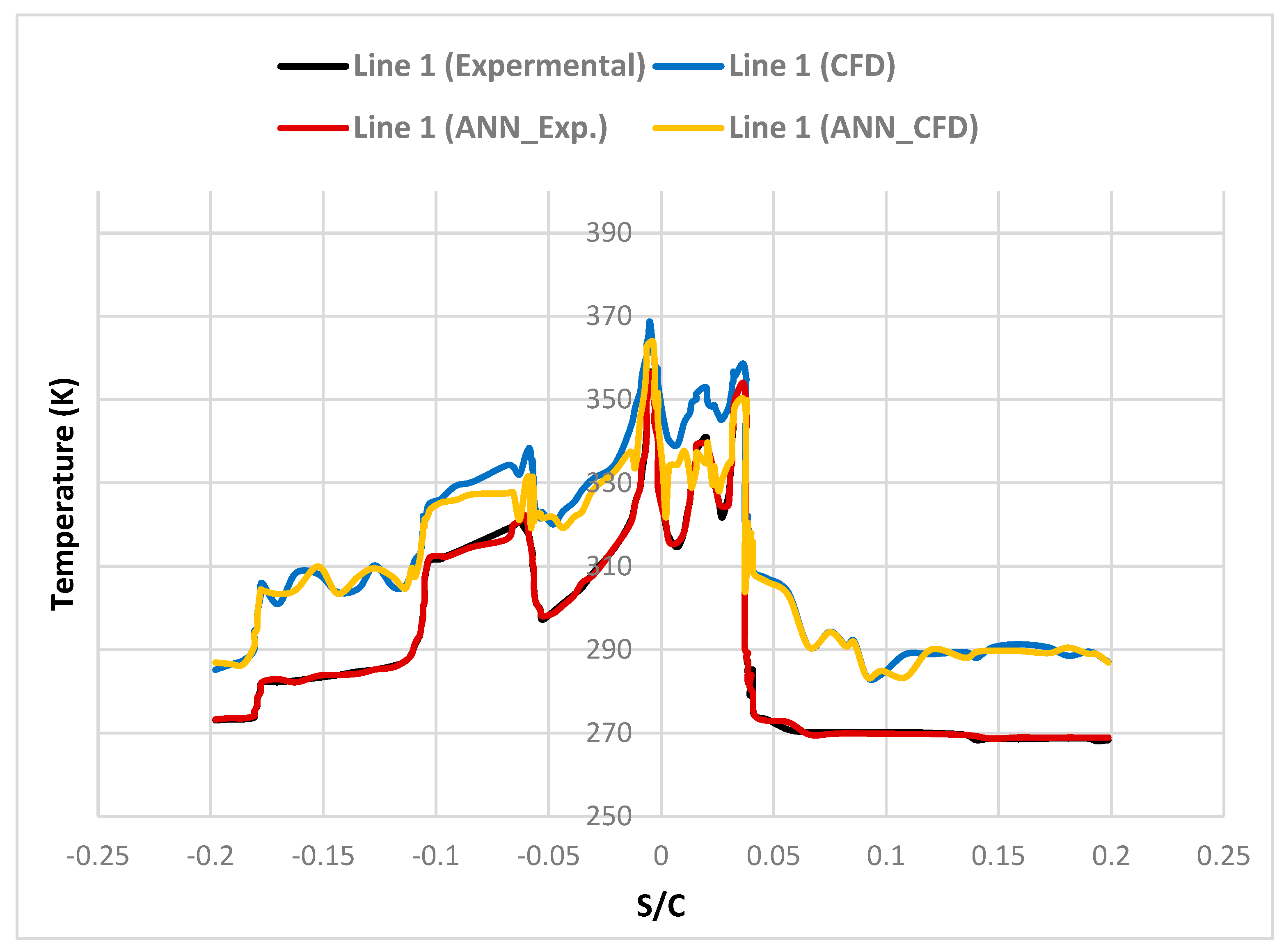
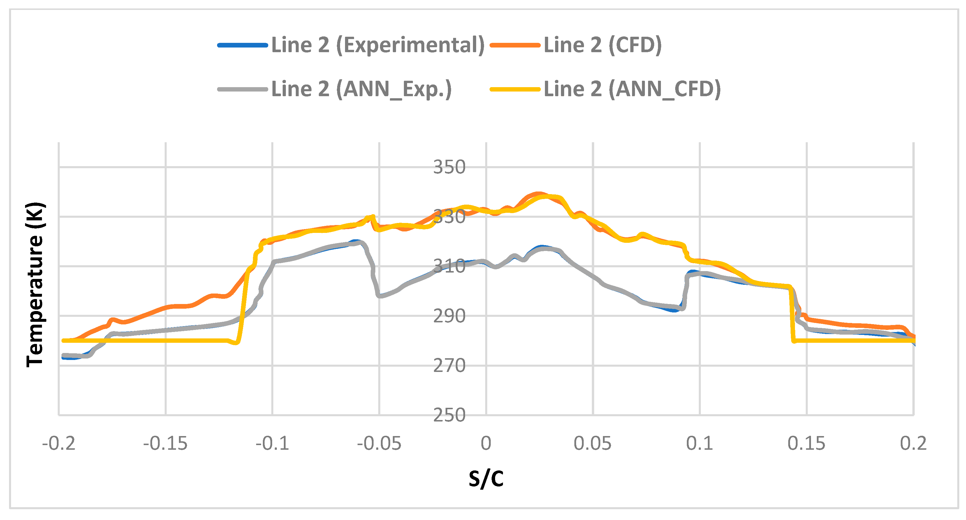
The temperatures along the three lines were predicted using the ANN models, and the results are presented in Figure 34, Figure 35 and Figure 36 for lines 1, 2, and 3, respectively. In Figure 34, there are four curves representing the temperature predictions of the obtained ANNs. These are the experimental temperature curve, ANN-predicted temperature based on experimental data (ANN_Exp.), temperature based on CFD simulation (CFD), and ANN-predicted temperature based on CFD data (ANN_CFD). The performance of the ANNs based on experimental and CFD data is evaluated using different performance metrics, including MAE, MSE, and R 2 . The results in Table 4 prove the efficiency of ANNs in the prediction of temperature when compared with the numerical CFD method. The table shows minimum values of MAE and MSE of around 6.06% and 0.72%, respectively, with the ANN models. In addition, the variance is near 1, which efficiently fits the experimental data through a trained network, in contrast with the results of CFD simulation, which has a variance of about 0.54. The results of the ANNs based on experimental data are closer to the experimental measurements than the results of the CFD simulation.
The results also show that the ANNs models based on the CFD data are closer to the experimental data than the CFD simulation results. For lines 2 and 3, the curves derived from the CFD simulation are different from those derived from the experimental data. However, the predictions from the ANN are very close to the experimental temperatures. The results show that the MAE for the ANNs has minimum values of around 6.06%, 4.34%, and 3.58% for lines 1, 2, and 3, respectively. Moreover, the minimum MSE values for the three lines are found with the ANN-based temperature predictions, at around 0.72%, 0.25%, and 0.684%, respectively. Finally, the ANN-predicted temperatures have very small errors and are almost the same as the experimental temperatures. In addition, the temperature curves for the ANNs based on CFD data and those for the CFD data are nearly the same, demonstrating that the two approaches perform very similarly. Figure 34, Figure 35 and Figure 36 alongside the performance metrics given in Table 4, show the calculated differences between the ANN and CFD results.

5.3. Scenario 3: IoT Based on ANNs

In the third scenario, the IoT is used to control and monitor the temperature of an aircraft wing via an anti-icing system. The IoT can make a suitable decision based on a certain threshold for the temperature. In addition, it can provide a visualization system for the temperature based on the data collected from the thermocouples. We implement the concept of the IoT using a commonly used platform, ThingSpeak.
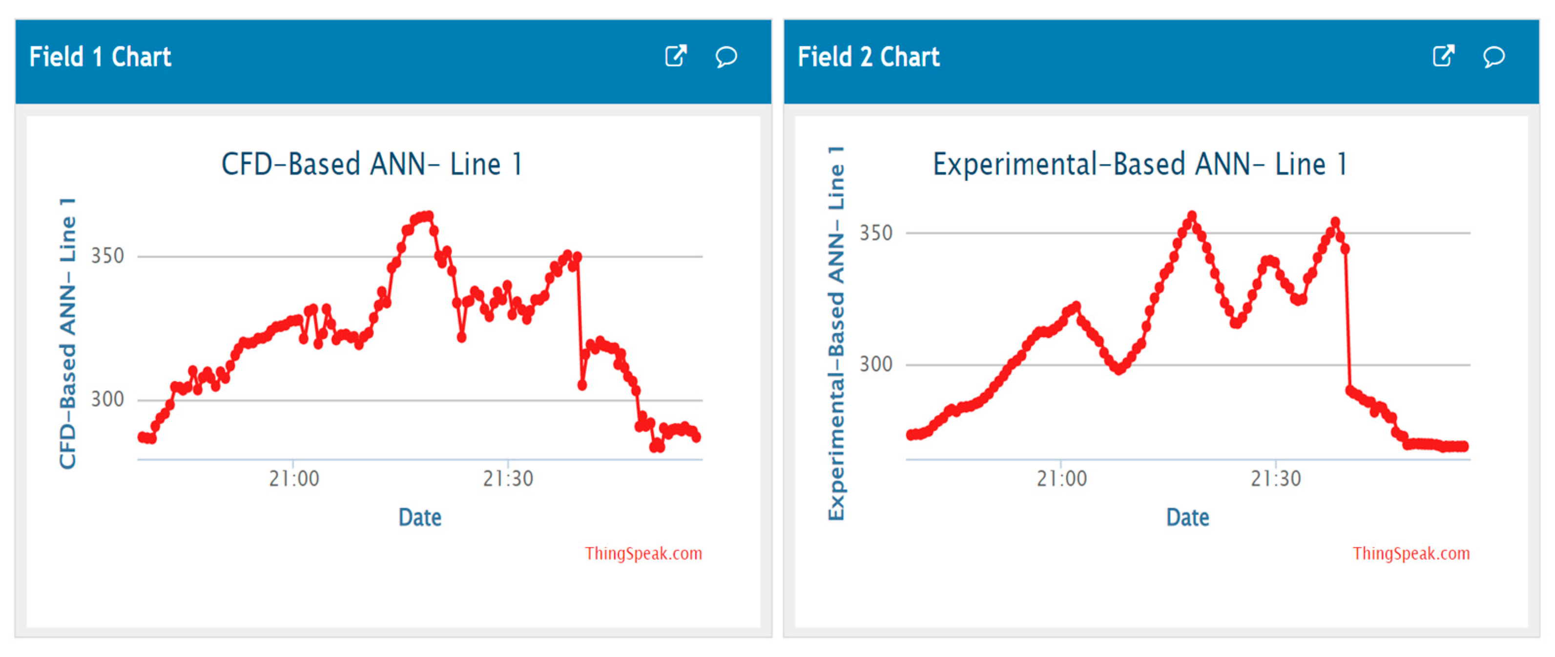
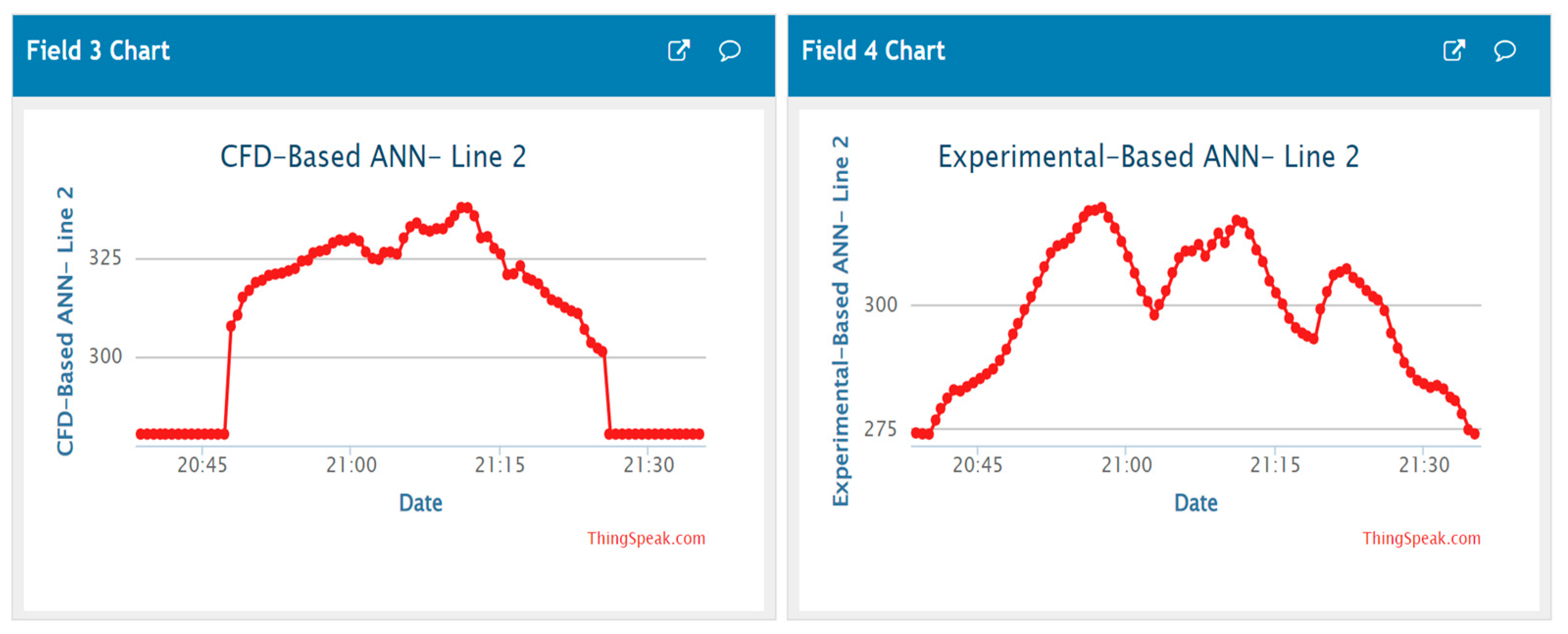
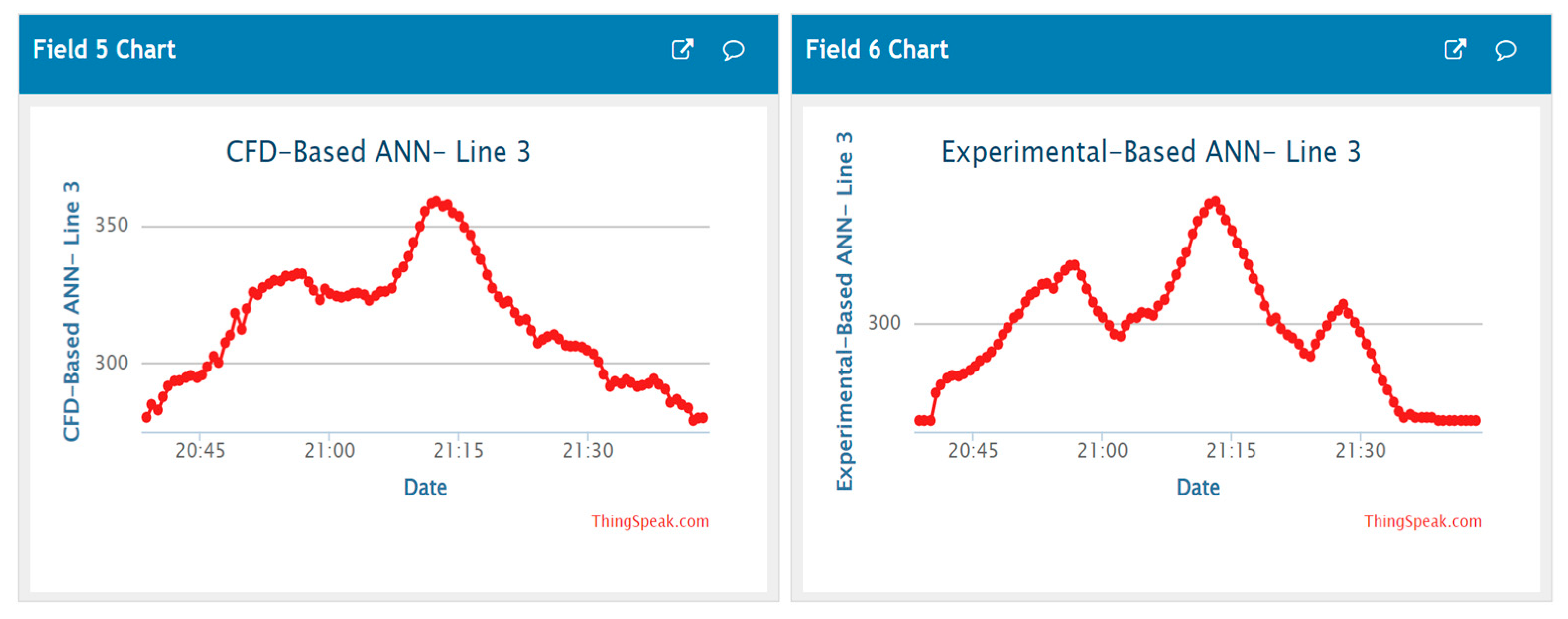
Thermocouple temperature sensors collect temperature measurements from three lines in an aircraft wing and these are used to build an ANN, which is then used to predict the temperature. These data are then published through an IoT platform (Figure 37, Figure 38 and Figure 39). Figure 37 demonstrates the predicted temperature for line 1 based on ANNs published through the IoT ThingSpeak platform in a private channel. In this figure, the figure on the right shows the predictions of an ANN model based on experimental data, while the figure on the left shows the predictions of an ANN model based on CFD data. Figure 38 and Figure 39 show the equivalent representations for line 2, and line 3, respectively.

6. Conclusions

In this study, the use of a neural network is proposed to build a prediction model of the temperature of an anti-icing system for an aircraft wing. In addition, the IoT was selected to monitor the temperature. The PSM of the wing anti-icing model constructed with the NACA 23014 airfoil is investigated. Various scenarios for verifying and validating the ANN and numerical CFD results with previous experimental thermocouple measurements are discussed. In the CFD analysis, a grid-independency check to decrease the number of grid elements without decreasing accuracy is investigated using the ANSYS software. The results of this test show that, after the seventh grid, the accuracy is almost unaffected by increasing the number of grid cells. Nine grids with about 2,666,876 cells are judged to be satisfactory for retaining accuracy while reducing the computation time of the solution. After a deep study, the results proved that there was a good agreement between ANN predictions and experimental measurements in all lines on the leading edge of the aircraft wing. They also show that the ANN predictions are much closer to experimental measurements than the CFD results, demonstrating that the neural network is a better tool for predicting the behavior of the system than a complicated and time-consuming tool such as CFD software. In future works, the effects of perturbations of flow, pressure, air temperature, and angle of attack will be taken into account to evaluate the performance of the ANN models. The domain size will also be studied. In addition, an experimental Hardware-in-the-Loop simulation will be implemented based on the IoT to emulate aircraft wing anti-icing systems with different fault scenarios, enabling the IoT platform to make suitable decisions based on the situation.

Author Contributions

Conceptualization, E.S.A., M.B.F. and M.E.-S.M.E.; methodology, M.E.-S.M.E.; software, E.S.A., M.B.F. and M.E.-S.M.E.; validation, E.S.A., M.E.-S.M.E. and M.M.A.; formal analysis, E.S.A., H.H.S., M.M.A. and M.B.F.; investigation, M.B.F., M.E.-S.M.E., H.H.S. and M.M.A.; resources, M.B.F. and M.M.A.; data curation, H.H.S.; writing—original draft preparation, M.E.-S.M.E., M.B.F. and E.S.A.; writing—review and editing, M.E.-S.M.E., M.B.F., M.M.A. and E.S.A.; visualization, M.E.-S.M.E., H.H.S. and M.M.A.; supervision, M.E.-S.M.E. and E.S.A.; project administration, E.S.A. and H.H.S.; funding acquisition, E.S.A. and H.H.S. All authors have read and agreed to the published version of the manuscript.

Funding

This research received no external funding.

Data Availability Statement

The data presented in this study are available on request from the corresponding authors.

Conflicts of Interest

The authors declare no conflict of interest.

References

  1. Abdelghany, E.S.; Sarhan, H.H.; Alahmadi, R.; Farghaly, M.B. Study the Effect of Winglet Height Length on the Aerodynamic Performance of Horizontal Axis Wind Turbines Using Computational Investigation. Energies 2023, 16, 5138. [Google Scholar] [CrossRef]
  2. Hamid, H.A.; Yong, W.K.; Yusoff, H.; Ismail, M.A. CFD Impingement Flow Study on Temperature Profile of Concave Plate. J. Adv. Res. Fluid Mech. Therm. Sci. 2022, 95, 1–16. [Google Scholar] [CrossRef]
  3. Li, B.; Sun, Q.; Xiao, D.; Zhang, W. Numerical Investigation of the Aerofoil Aerodynamics with Surface Heating for Anti-Icing. Aerospace 2022, 9, 338. [Google Scholar] [CrossRef]
  4. Fukudome, K.; Tomita, Y.; Uranai, S.; Mamori, H.; Yamamoto, M. Evaluation of Anti-Icing Performance for an NACA0012 Airfoil with an Asymmetric Heating Surface. Aerospace 2021, 8, 294. [Google Scholar] [CrossRef]
  5. Broeren, A.P.; Potapczuk, M.G.; Riley, J.T.; Villedieu, P.; Moëns, F.; Bragg, M.B. Swept-Wing Ice Accretion Characterization and Aerodynamics. In Proceedings of the 2011 Annual Technical Meeting, St. Louis, MO, USA, 10–12 May 2011; AIAA: Reston, VA, USA, 2013; pp. 2013–2824. [Google Scholar] [CrossRef] [Green Version]
  6. Hedde, T.; Guffond, D. ONERA three-dimensional icing model. AIAA J. 1995, 33, 1038–1045. [Google Scholar] [CrossRef]
  7. Li, H.; Hu, Q.; Jiang, X.; Yu, Z.; Shu, L.; Li, C.; Qiu, Z. Review on Anti-icing and De-icing Techniques of Wind Turbine Blades. In Proceedings of the IWAIS 2022, Montreal, QC, Canada, 19–23 June 2022. [Google Scholar]
  8. Michael, P.; Wong, S.-H.; Yeong, H.-W.; Wong, S.-C.; Vu, G.T. Experimental Investigation of a Bleed Air Ice Protection System. SAE Trans. 2007, 116, 643–663. Available online: http://www.jstor.org/stable/44719498 (accessed on 1 January 2007).
  9. Subramaniam, R.; Keith, T.G.; De Witt, K.J.; Putt, J.C.; Mailing, C.A.; Leffel, K.L. Numerical modeling of an advanced pneumatic impulse ice protection system for aircraft. J. Aircr. 1992, 29, 1057–1063. [Google Scholar] [CrossRef]
  10. Robert, I.E.; Schrag, R.L.; Bernhart, W.D.; Zumwalt, G.W.; Kendrew, T.J. An investigation of power line de-icing by electro-impulse methods. IEEE Trans. Power Deliv. 1989, 4, 1855–1861. [Google Scholar] [CrossRef]
  11. Hassaani, A.; Elsayed, A.F.; Khalil, E.E. Numerical investigation of thermal anti-icing system of aircraft wing. Int. Robot. Autom. J. 2020, 6, 60–65. [Google Scholar] [CrossRef]
  12. Avi, A. Development of Icing Testing Tools for Large Climatic Chamber. Master Thesis, School of Industrial and Information Engineering, Politecnico di Milano University, Milano, Italy, 2020. [Google Scholar]
  13. Brown, J.M.; Raghunathan, S.; Watterson, J.K.; Linton, A.J.; Riordon, D. Heat transfer correlation for anti-icing systems. J. Aircr. 2002, 39, 65–70. [Google Scholar] [CrossRef]
  14. Li, R.; Zhu, G.; Zhang, D. Investigation on the Mechanism of Heat Load Reduction for the Thermal Anti-Icing System. Energies 2020, 13, 5911. [Google Scholar] [CrossRef]
  15. Uranai, S.; Fukudome, K.; Mamori, H.; Fukushima, N.; Yamamoto, M. Numerical Simulation of the Anti-Icing Performance of Electric Heaters for Icing on the NACA 0012 Airfoil. Aerospace 2020, 7, 123. [Google Scholar] [CrossRef]
  16. Asaumi, N.; Mizuno, M.; Tomioka, Y.; Suzuki, K.; Hyugaji, T.; Kimura, S. Experimental Investigation and Simple Estimation of Heat Requirement for Anti-Icing. J. Gas Turbine Soc. Jpn. 2018, 46, 476–485. [Google Scholar] [CrossRef]
  17. De Mattos, B.; Oliveira, G. Three-dimensional Coupled Analysis of a Wing Slice Slat with a Piccolo Tube. In Proceedings of the 18th Applied Aerodynamics Conference, Denver, CO, USA, 14–17 August 2000; p. 3921. [Google Scholar] [CrossRef]
  18. Wong, S.-H.; Zamora, A. Computational Investigation of a Bleed Air Ice Protection System. In Proceedings of the 1st AIAA Atmospheric and Space Environments Conference, San Antonio, TX, USA, 22–25 June 2009; AIAA: Reston, VA, USA, 2009. [Google Scholar]
  19. Lima, D.S.G.A.; Otávio, D.M.S.; Godoy, D.J.Z.E.J. Numerical simulation of airfoil thermal anti-ice operation, part 1: Mathematical modelling. J. Aircr. 2007, 44, 627–633. [Google Scholar] [CrossRef]
  20. Liu, H.H.T.; Hua, J. Three-dimensional integrated thermodynamic simulation for wing anti-icing system. J. Aircr. 2004, 41, 1291–1297. [Google Scholar] [CrossRef]
  21. Cheng, J.-C.; Chen, Y.-M. Investigation of fluid flow and heat transfer characteristics for a thermal anti-icing system of a high-altitude and long-endurance UAV. J. Mech. 2021, 37, 467–483. [Google Scholar] [CrossRef]
  22. Choi, M.; Yoo, H.S.; Yang, G.; Lee, J.S.; Sohn, D.K. Measurements of impinging jet flow and heat transfer on a semi-circular concave surface. Int. J. Heat Mass Transf. 2000, 43, 1811–1822. [Google Scholar] [CrossRef]
  23. Wright, W.B. An Evaluation of Jet Impingement Heat Transfer Correlations for Piccolo Tube Application. In Proceedings of the 42nd AIAA Aerospace Sciences Meeting and Exhibit, Reno, NV, USA, 5–8 January 2004. [Google Scholar]
  24. Sreedharan, C.; Nagpurwala, Q.; Subbaramu, H.S. Effect of Hot Air Jets from a Piccolo Tube in Aircraft Wing Anti-Icing Unit. MSRUAS-SASTech J. 2014, 13, 2–5. [Google Scholar]
  25. Zhou, S.; Liu, X.; Du, G.; Liu, C.; Zhou, Y. Comparison study of CFD and artificial neural networks in predicting temperature fields induced by natural convention in a square enclosure. Therm. Sci. 2019, 23, 3481–3492. [Google Scholar] [CrossRef]
  26. Rubio, G.; Valero, E.; Lanzan, S. Computational Fluid Dynamics Expert System using Artificial Neural Networks. Int. J. Comput. Inf. Eng. 2012, 6, 413–417. [Google Scholar]
  27. Gholami, A.; Bonakdari, H.; Akhtari, A.A.; Ebtehaj, I. A combination of computational fluid dynamics, artificial neural network, and support vectors machines models to predict flow variables in curved channel. Sci. Iran. 2019, 26, 726–741. [Google Scholar] [CrossRef] [Green Version]
  28. Chang, S.; Leng, M.; Wu, H.; Thompson, J. Aircraft ice accretion prediction using neural network and wavelet packet transform. Aircr. Eng. Aerosp. Technol. Int. J. 2016, 88, 128–136. [Google Scholar] [CrossRef]
  29. Kuan, Y.; Lien, H. The integration of the neural network and computational fluid dynamics for the heatsink design. In Proceedings of the Advances in Neural Networks–ISNN 2005: Second International Symposium on Neural Networks, Chongqing, China, 30 May–1 June 2005; Proceedings, Part III 2. Springer: Berlin/Heidelberg, Germany; pp. 933–938. [Google Scholar]
  30. Strijhak, S.; Ryazanov, D.; Koshelev, K.; Ivanov, A. Neural Network Prediction for Ice Shapes on Airfoils Using iceFoam Simulations. Aerospace 2022, 9, 96. [Google Scholar] [CrossRef]
  31. Jung, S.K.; Shin, S.; Myong, R.S.; Cho, T.H. An efficient CFD-based method for aircraft icing simulation using a reduced order model. J. Mech. Sci. Technol. 2011, 25, 703–711. [Google Scholar] [CrossRef]
  32. Sadrehaghighi, I. Artificial Neutral Networks (ANNs) Applied as CFD Optimization Techniques; Springer Nature: Berlin, Germany, 2021. [Google Scholar]
  33. Georgieva, P.; De Azevedo, S.F. Neural network-based control strategies applied to a fed-batch crystallization process. Int. J. Chem. Mol. Eng. 2007, 1, 145–154. [Google Scholar]
  34. Yi, X.; Wang, Q.; Chai, C. Prediction model of aircraft icing based on deep neural network. Trans. Nanjing Univ. Aeronaut. Astronaut. 2021, 38, 535–544. [Google Scholar]
  35. Shora, M.M.; Ghassemi, H.; Nowruzi, H. Using computational fluid dynamic and artificial neural networks to predict the performance and cavitation volume of a propeller under different geometrical and physical characteristics. J. Mar. Eng. Technol. 2018, 17, 59–84. [Google Scholar] [CrossRef]
  36. Essa, M.E.S.M.; Lotfy, J.V.W.; Abd-Elwahed, M.E.K.; Rabie, K.; ElHalawany, B.M.; Elsisi, M. Low-cost hardware in the loop for intelligent neural predictive control of hybrid electric vehicle. Electronics 2023, 12, 971. [Google Scholar] [CrossRef]
  37. Essa, M.E.S.M.; Elsisi, M.; Saleh Elsayed, M.; Fawzy Ahmed, M.; Elshafeey, A.M. An Improvement of Model Predictive for Aircraft Longitudinal Flight Control Based on Intelligent Technique. Mathematics 2022, 10, 3510. [Google Scholar] [CrossRef]
  38. Essa, M.E.S.M.; El-shafeey, A.M.; Omar, A.H.; Fathi, A.E.; Maref, A.S.A.E.; Lotfy, J.V.W.; El-Sayed, M.S. Reliable Integration of Neural Network and Internet of Things for Forecasting, Controlling, and Monitoring of Experimental Building Management System. Sustainability 2023, 15, 2168. [Google Scholar] [CrossRef]
  39. Sabancı, K.; Yigit, E.; Üstün, D.; Toktaş, A.; Çelik, Y. Thingspeak based monitoring IoT system for counting people in a library. In Proceedings of the 2018 International Conference on Artificial Intelligence and Data Processing (IDAP), Malatya, Turkey, 28–30 September 2018; IEEE: Washington, DC, USA; pp. 1–6. [Google Scholar]
  40. Deekshath, R.; Dharanya, P.; Kabadia MK, D.; Dinakaran MG, D.; Shanthini, S. IoT based environmental monitoring system using arduino UNO and thingspeak. Int. J. Sci. Technol. Eng. 2018, 4, 68–75. [Google Scholar]
  41. Razali, M.A.A.; Kassim, M.; Sulaiman, N.A.; Saaidin, S. A thingspeak IoT on real time room condition monitoring system. In Proceedings of the 2020 IEEE International Conference on Automatic Control and Intelligent Systems (I2CACIS), Shah Alam, Malaysia, 20–20 June 2020; IEEE: Washington, DC, USA; pp. 206–211. [Google Scholar]
  42. Pasha, S. ThingSpeak based sensing and monitoring system for IoT with Matlab Analysis. Int. J. New Technol. Res. 2016, 2, 19–23. [Google Scholar]
  43. Zhu, Z.; Li, Y.; Gong, S. Design and experiment of IOT cooling system in glass greenhouse based on CFD simulation. J. Agric. Eng. 2023. [Google Scholar] [CrossRef]
  44. Değerli, M.C.; Şahin, Ö.; Yazar, I.; Kuşhan, M.C. Internet of Things in Maintenance and Virtual Reality/Augmented Reality Applications in Aircraft Maintenance. International Maintenance Technologies Congress and Exhibition; Pamukkale University Congress and Cultural Center: Denizli, Türkiye, 2022. [Google Scholar]
  45. Duhovnikov, S.; Baltaci, A.; Gera, D.; Schupke, D.A. Power consumption analysis of NB-IoT technology for low-power aircraft applications. In Proceedings of the 2019 IEEE 5th World Forum on Internet of Things (WF-IoT), Limerick, Ireland, 15–18 April 2019; IEEE: Washington, DC, USA; pp. 719–723. [Google Scholar]
  46. Salman, L.; Salman, S.; Jahangirian, S.; Abraham, M.; German, F.; Blair, C.; Krenz, P. Energy efficient IoT-based smart home. In Proceedings of the 2016 IEEE 3rd World Forum on Internet of Things (WF-IoT), Reston, VA, USA, 12–14 December 2016; IEEE: Washington, DC, USA; pp. 526–529. [Google Scholar]
  47. Khalil, E.E.; Abdelattif, O.E.; Abdel Ghany, E.S.; El Hariri, G.A. Computational Analyses of Aerodynamic Characteristics of NACA653218airfoil. In Proceedings of the 54th AIAA Aerospace Sciences Meeting, San Diego, CA, USA, 4–8 January 2016; p. 1367. [Google Scholar] [CrossRef]
  48. Saeed, F.; Ahmed, K.Z.; Owes, A.O.E.; Paraschivoiu, I. Anti-icing hot air jet heat transfer augmentation employing inner channels. Adv. Mech. Eng. 2021, 13, 1–13. [Google Scholar] [CrossRef]
  49. Abdelghany, E.S.; Khalil, E.E.; Abdellatif, O.E.; ElHarriri, G. Winglet Cant and Sweep Angles Effect on Aircraft Wing Performance. In Proceedings of the 17th International Conference on Applied Mechanics and Mechanical Engineering, Cairo, Egypt, 19–21 April 2016; Military Technical College, Kobry El-Kobbah: Cairo, Egypt, 2016; Volume 17, pp. 1–17. [Google Scholar]
  50. Abdelghany, E.S.; Sarhan, H.H.; El Saleh, A.; Farghaly, M.B. High bypass turbofan engine and anti-icing system performance: Mass flow rate of anti-icing bleed air system effect. Case Stud. Therm. Eng. 2023, 45, 102927. [Google Scholar] [CrossRef]
  51. Hannat, R.; Morency, F. Numerical Validation of Conjugate Heat Transfer Method for Anti-/De-Icing Piccolo System. J. Aircr. 2014, 51, 104–116. [Google Scholar] [CrossRef]
  52. Farghaly, M.B.; Abdelghany, E.S. Study the effect of trailing edge flap deflection on horizontal axis wind turbine performance using computational investigation. Int. J. Renew. Energy Res. (IJRER) 2022, 12, 1942–1953. [Google Scholar] [CrossRef]
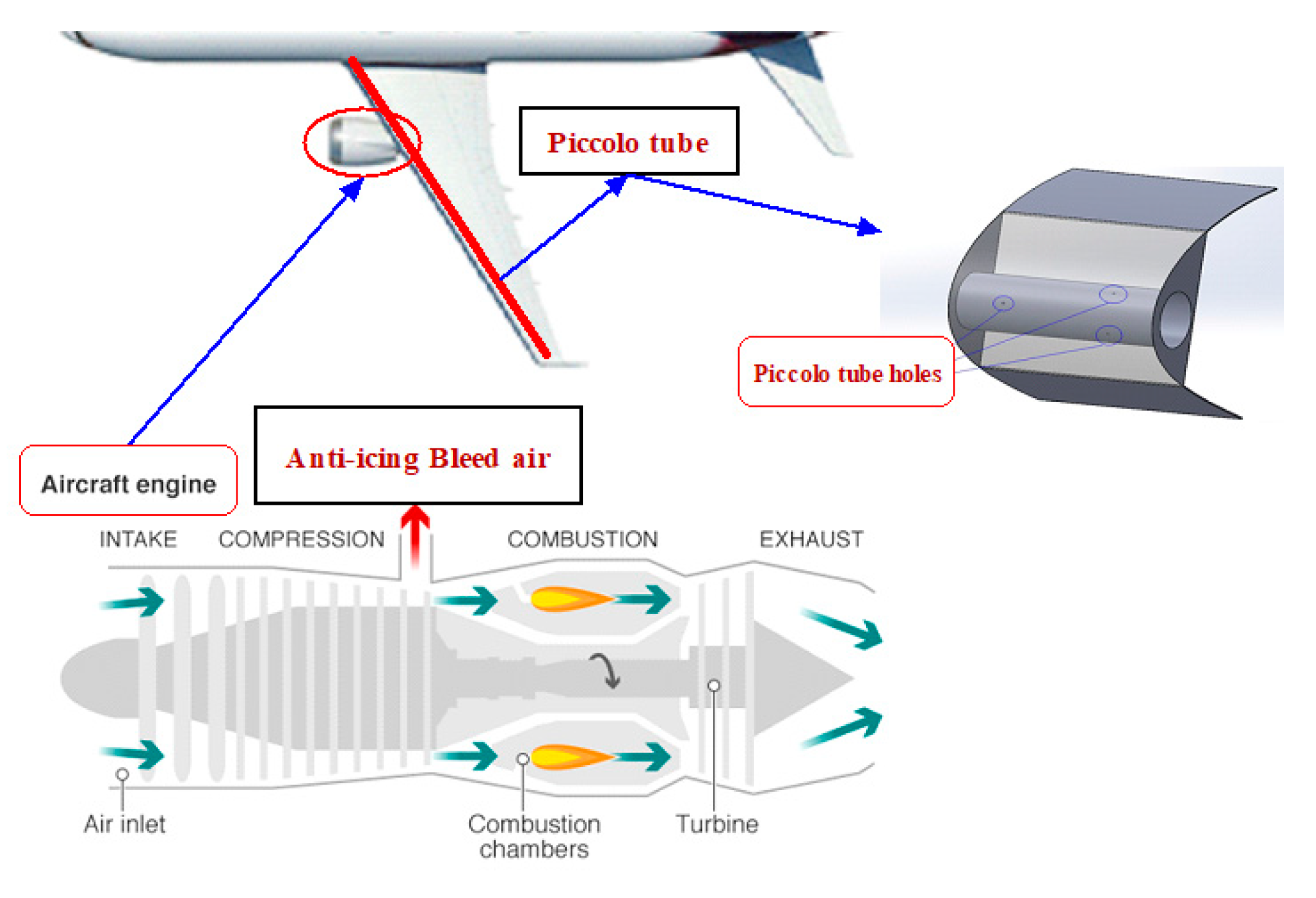
Figure 1. Schematic of the use of engine bleed air in a wing anti-icing system via a piccolo tube.
Aerospace 10 00676 g001
Figure 2. The three phases of generating the wing anti-icing system CFD model.
Aerospace 10 00676 g002
Figure 3. The wing anti-icing system computational domain dimensions: (a) external flow domain and (b) internal flow domain parameters.
Aerospace 10 00676 g003
Figure 4. The wing anti-icing system computational internal and external flow domains boundary conditions.
Aerospace 10 00676 g004
Figure 5. The flow chart of the anti-icing model simulation.
Aerospace 10 00676 g005
Figure 6. Wing anti-icing system external and internal flow domain meshing.
Aerospace 10 00676 g006
Figure 7. Proposed structure of ANN based on IoT for aircraft wing anti-icing system.
Aerospace 10 00676 g007
Figure 8. Wing anti-icing system temperature measurement using three lines of thermocouples.
Aerospace 10 00676 g008
Figure 9. Curves of temperature distribution (K) against the number of grid cells for (a) line 1, (b) line 2, and (c) line 3.
Aerospace 10 00676 g009aAerospace 10 00676 g009b
Figure 10. Numerical and experimental results, temperature distribution in (K): (a) line 1, (b) line 2, and (c) line 3.
Aerospace 10 00676 g010aAerospace 10 00676 g010b
Figure 11. Computational wing anti-icing system contours: (a) streamlines of internal flow domain (m/s), (b) heat flux contours on wing outer surface (W·m2), (c) temperature contours on wing inner surface, and (d) temperature contours on wing outer surface.
Aerospace 10 00676 g011aAerospace 10 00676 g011b
Figure 12. Shape of the velocity streamlines of the internal and external coupled flow domains, (A) internal flow domain, and (B) external flow domain.
Aerospace 10 00676 g012
Figure 13. The velocity contours of the internal and external coupled flow domains, (A) internal flow domain, and (B) external flow domain.
Aerospace 10 00676 g013
Figure 14. Temperature contours of the internal and external coupled flow domains.
Aerospace 10 00676 g014
Figure 15. Structure of ANN for forecasting temperature.
Aerospace 10 00676 g015
Figure 16. Training performance of ANN for line 1 based on experimental data.
Aerospace 10 00676 g016
Figure 17. Training regression of ANN for line 1 based on experimental data.
Aerospace 10 00676 g017
Figure 18. Training state of ANN for line 1 based on experimental data.
Aerospace 10 00676 g018
Figure 19. Training performance of ANN for line 1 based on CFD data.
Aerospace 10 00676 g019
Figure 20. Training regression of ANN for line 1 based on CFD data.
Aerospace 10 00676 g020
Figure 21. Training state of ANN for line 1 based on CFD data.
Aerospace 10 00676 g021
Figure 22. Training performance of ANN for line 2 based on experimental data.
Aerospace 10 00676 g022
Figure 23. Training regression of ANN for line 2 based on experimental data.
Aerospace 10 00676 g023
Figure 24. Training state of ANN for line 2 based on experimental data.
Aerospace 10 00676 g024
Figure 25. Training performance of ANN for line 2 based on CFD data.
Aerospace 10 00676 g025
Figure 26. Training regression of ANN for line 2 based on CFD data.
Aerospace 10 00676 g026
Figure 27. Training state of ANN for line 2 based on CFD data.
Aerospace 10 00676 g027
Figure 28. Training performance of ANN for line 3 based on experimental data.
Aerospace 10 00676 g028
Figure 29. Training regression of ANN for line 3 based on experimental data.
Aerospace 10 00676 g029
Figure 30. Training state of ANN for line 3 based on experimental data.
Aerospace 10 00676 g030
Figure 31. Training performance of ANN for line 3 based on CFD data.
Aerospace 10 00676 g031
Figure 32. Training regression of ANN for line 3 based on CFD data.
Aerospace 10 00676 g032
Figure 33. Training state of ANN for line 3 based on CFD data.
Aerospace 10 00676 g033
Figure 34. Comparison between ANNs and CFD for line 1.
Aerospace 10 00676 g034
Figure 35. Comparison between ANNs and CFD for line 2.
Aerospace 10 00676 g035
Figure 36. Comparison between ANNs and CFD for line 3.
Aerospace 10 00676 g036
Figure 37. Monitoring of predicted temperature for line 1 based on IoT ThingSpeak.
Aerospace 10 00676 g037
Figure 38. Monitoring of predicted temperature for line 2 based on IoT ThingSpeak.
Aerospace 10 00676 g038
Figure 39. Monitoring of predicted temperature for line 3 based on IoT ThingSpeak.
Aerospace 10 00676 g039
Table 1. Boundary conditions for computational domains.
External Flow DomainInternal Flow Domain
Inlet air velocity59.2 m/sMass flow of hot air jets ( m ˙ )0.327 g/s
Temperature of external flow268.21 KTemperature of hot air jets 449.82 K
AOA3 degreesTemperature of piccolo tube wall449.82 K
Density0.9031 kg/m3H9.01 mm
Dynamic Viscosity1.692 × 10−5 N s/m2α45 degrees
Altitude above Sea Level3069.34 m
Table 2. Nine kinds of meshes with each sub-domain and total elements for wing anti-icing system.
No.Grid(1)Grid(2)Grid(3)Grid(4)Grid(5)Grid(6)Grid(7)Grid(8)Grid(9)
External Domain Elements166,140364,470364,470364,470520,500658,250658,250658,250685,250
Solid Domain Elements12,34819,48819,48819,48828,56028,56028,56028,56028,560
Internal Domain Elements164,3191,024,4131,085,2521,259,0101,477,1811,477,1811,608,8001,777,5851,953,066
Total Elements342,8071,408,3711,469,2101,642,9682,026,2412,163,9912,295,6102,464,3952,666,876
Table 3. Performance data of neural networks for line 1, line 2, and line 3 based on CFD and experimental (Exp.) data.
ANNSamplesMSERegressionPerformance
Line 1Exp.Training14211.121.00.977
Validation3041.011.0
Testing3041.181.0
CFDTraining14212.501.02.13
Validation3042.611.0
Testing3042.781.0
Line 2Exp.Training14153.16 × 10−21.02.08
Validation3033.51 × 10−21.0
Testing3033.89 × 10−21.0
CFDTraining14152.617 × 10−11.03.9
Validation3032.683 × 10−11.0
Testing3032.647 × 10−11.0
Line 3Exp.Training14112.65 × 10−11.0156
Validation3032.75 × 10−11.0
Testing3032.72 × 10−11.0
CFDTraining14111.16 × 10−21.00.624
Validation3031.11 × 10−21.0
Testing3031.36 × 10−21.0
Table 4. Performance metrics for the three lines for the CFD and ANN approaches.
Line 1Line 2Line 3
TypeCFDANN-CFDANN-EXP.CFDANN-CFDANN-EXP.CFDANN-CFDANN-EXP.
Performance
MAE (%)40.0924.496.0659.6938.54.3438.474.293.58
MSE (%)22.695.820.7227.365.650.2523.50.6820.684
R20.540.990.990.530.930.9980.560.9980.998
Disclaimer/Publisher’s Note: The statements, opinions and data contained in all publications are solely those of the individual author(s) and contributor(s) and not of MDPI and/or the editor(s). MDPI and/or the editor(s) disclaim responsibility for any injury to people or property resulting from any ideas, methods, instructions or products referred to in the content.