Article

Nonlinear Time Series Analysis and Prediction of General Aviation Accidents Based on Multi-Timescales

1
College of Civil Aviation, Nanjing University of Aeronautics and Astronautics, Nanjing 211106, China
2
National Key Laboratory of Air Traffic Flow Management, Nanjing University of Aeronautics and Astronautics, Nanjing 211106, China
*
Author to whom correspondence should be addressed.
Aerospace 2023, 10(8), 714; https://doi.org/10.3390/aerospace10080714
Submission received: 20 June 2023 / Revised: 6 August 2023 / Accepted: 13 August 2023 / Published: 16 August 2023
(This article belongs to the Section Air Traffic and Transportation)

Abstract

:
General aviation accidents have complex interactions and influences within them that cannot be simply explained and predicted by linear models. This study is based on chaos theory and uses general aviation accident data to conduct research on different timescales (HM-scale, ET-scale, and EF-scale). First, time series are constructed by excluding seasonal patterns from the statistics of general aviation accidents. Secondly, the chaotic properties of multi-timescale series are determined by the 0–1 test and Lyapunov exponent. Finally, by introducing the sparrow search algorithm and tent chaotic mapping, a CSSA-LSSVM prediction model is proposed. The accident data of the National Transportation Safety Board (NTSB) of the United States in the past 15 years is selected for case analysis. The results show that the phase diagram of the 0–1 test presents Brownian motion characteristics, and the maximum Lyapunov exponents of the three scales are all positive, proving the chaotic characteristics of multi-timescale series. The CSSA-LSSVM prediction model’s testing results illustrate its superiority in time series predicting, and when the timescale declines, the prediction error reduces gradually while the fitting effect strengthens and then decreases. This study uncovers the nonlinear chaotic features of general aviation accidents and demonstrates the significance of multi-timescale research in time series analysis and prediction.

1. Introduction

Accident [1] is an occurrence associated with the operation of an aircraft that takes place during the period from when individuals board an aircraft with the intention of flight until all passengers have disembarked, which include injury or death of personnel, damage to or structural failure of the aircraft, the disappearance of the aircraft, or total inaccessibility. It is a complex nonlinear phenomenon resulting from the combined effects of inherent complexity and dynamics, presenting complex correlation characteristics such as diverse types and mutual influence. While incidents can have an impact on general aviation operations, they seldom result in major harm or loss. Conversely, accidents can result in serious damage, injuries, loss of life, or the destruction of an aircraft. As a result, we concentrate on researching accident data to better understand the hazards and challenges of general aviation. Research and study of general aviation accident historical data, which can uncover hidden patterns and analyze data regulations, serve as theoretical support and a scientific basis for safety situational awareness. Furthermore, the research on accident time series prediction helps in the identification of hazards, trends, and critical risk periods. It offers essential information for accident prevention, allows for accurate execution of safety management measures, reduces the probability of accidents, and improves air traffic safety by establishing more accurate and efficient safety processes, ultimately increasing general aviation’s overall safety level.
Concerning the study of aviation accidents in terms of modeling and forecasting, the research team of He et al. [2] conducted an examination of the aspects impacting airline accidents and employed time-based evaluation approaches such as intercorrelation analysis, cointegration analysis, and causal analysis to study the connection between airline accidents and airline capacity. Bao [3] and Kenneth D. et al. [4] analyzed causal factors and themes affecting aviation safety based on textual data mining of unsafe civil aviation events to explore embedded correlations and hidden connections. Rosa et al. [5] constructed a statistical estimation and prediction model through a Bayesian algorithm and hierarchical structure to predict future safety performance and risk. With the use of the NLMS algorithm, Wang et al. [6] built a Volterra series model to estimate the yearly accident rate in aviation. They then predicted the number of U.S. Air Force flying accidents per ten thousand hours. Yu et al. [7] used the chaos analysis method to reconstruct the sequence of aircraft accidents and used the CSVR model of the support vector machine for prediction. Ni et al. [8] proposed a prediction method for serious flight accident rates based on deep learning, considering big data characteristics. They predicted the rate of serious airplane accidents by combining principal component analysis (PCA) and deep belief networks (DBN). At present, relevant research mainly focuses on correlation analysis of influencing factors, accident text mining and risk identification, causation statistical inference, accident occurrence number prediction, and so on, with few scholars having studied the time series characteristics, intrinsic occurrence mechanism, and development trend regularity of historical data on general aviation accidents.
Regarding the analysis and prediction research of nonlinear time series, it has been widely applied in time series dynamics fields such as geological change prediction [9], power load forecasting [10], financial market forecasting [11], traffic flow forecasting [12], and so on. Wang et al. [13], based on traffic flow time series, improved the CAO method to determine the reconstructed phase space embedding dimension value, and used a genetic algorithm to optimize the RBF neural network to predict the reconstructed time series. Li et al. [14] studied regional air route network traffic status, analyzed the chaotic characteristics of traffic volume time series, and predicted traffic volume change trends. Cheng et al. [15] used chaos theory to discover chaotic aspects of traffic flow, such as factors related to speed, occupancy, and flow, and predicted traffic flow using support vector regression (SVR) models. Numerical experiments are conducted on multi-source data. In terms of nonlinear time series prediction methods, there are mainly Bayesian network prediction model-based methods, gray interval prediction models, and BP neural network-based machine learning algorithm models. At present, there are problems such as low prediction accuracy of models or algorithms themselves and high complexity in the iterative calculation process.
To solve those problems, our study mines historical data from general aviation accidents using the National Transportation Safety Board Database for the past 15 years. The main contributions of this paper are as follows:
(1)
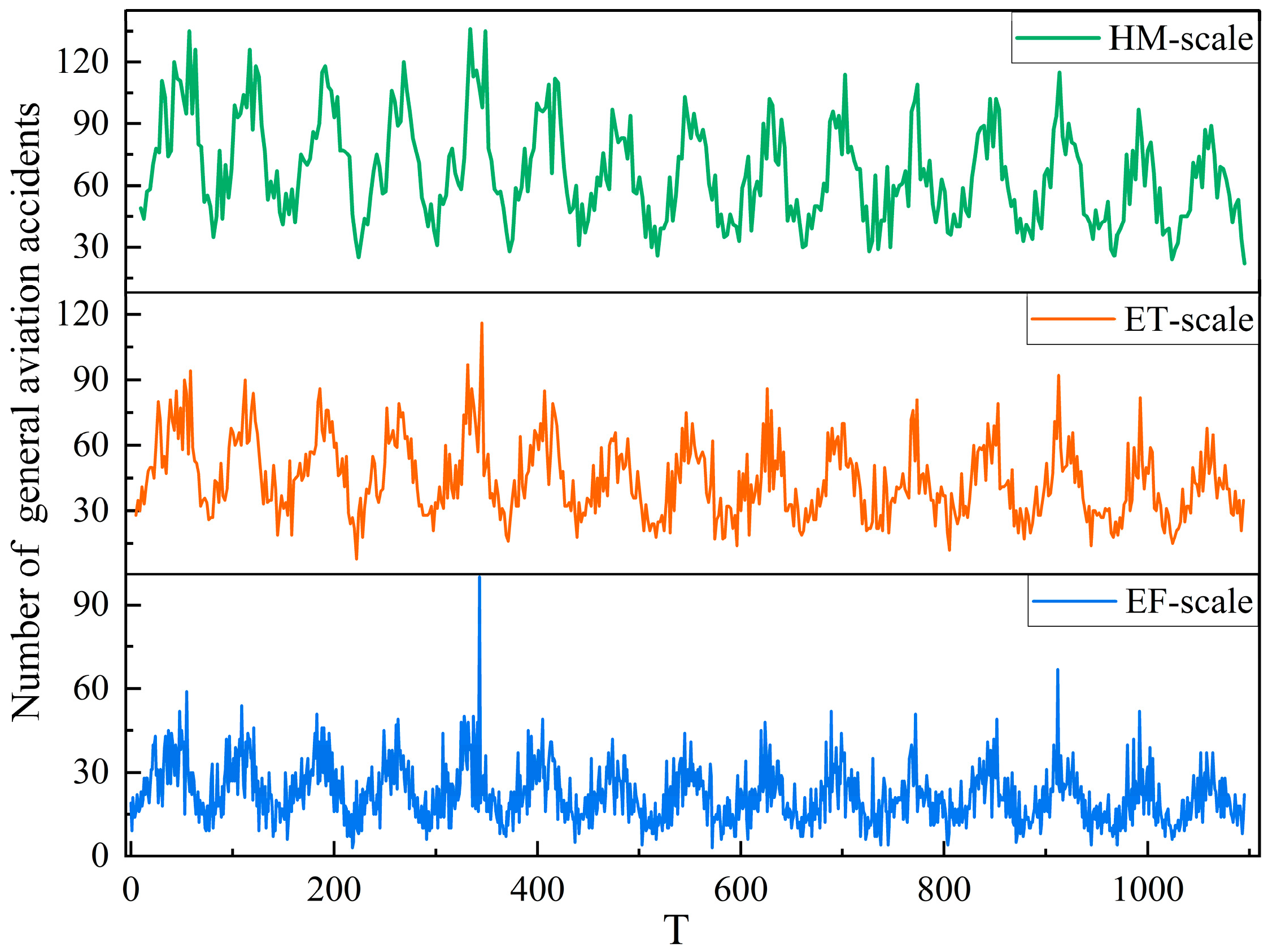
With a focus on understanding the time series features of accidents and constructing time series on multiple scales, the periodic variation factors of three scale subseries (EF-, ET-, and HM-) are eliminated using seasonal decomposition. The 0–1 test, phase space reconstruction, and Lyapunov exponent are used to investigate the intrinsic dynamical and chaotic features of the multi-timescale series.
(2)
Based on the results of the multi-timescale series chaotic characteristics analysis of general aviation accidents, the chaotic sparrow search algorithm is used to optimize the parameters of the LSSVM model, and an improved prediction model for the CSSA-LSSVM model is presented.
(3)
Using simulation experiments to prove the rationality of the above methodologies and predict the development trend of general aviation safety, potential risks can be identified in an immediate response by analyzing general aviation accident time series predictions, which is crucial to enhancing general aviation safety.
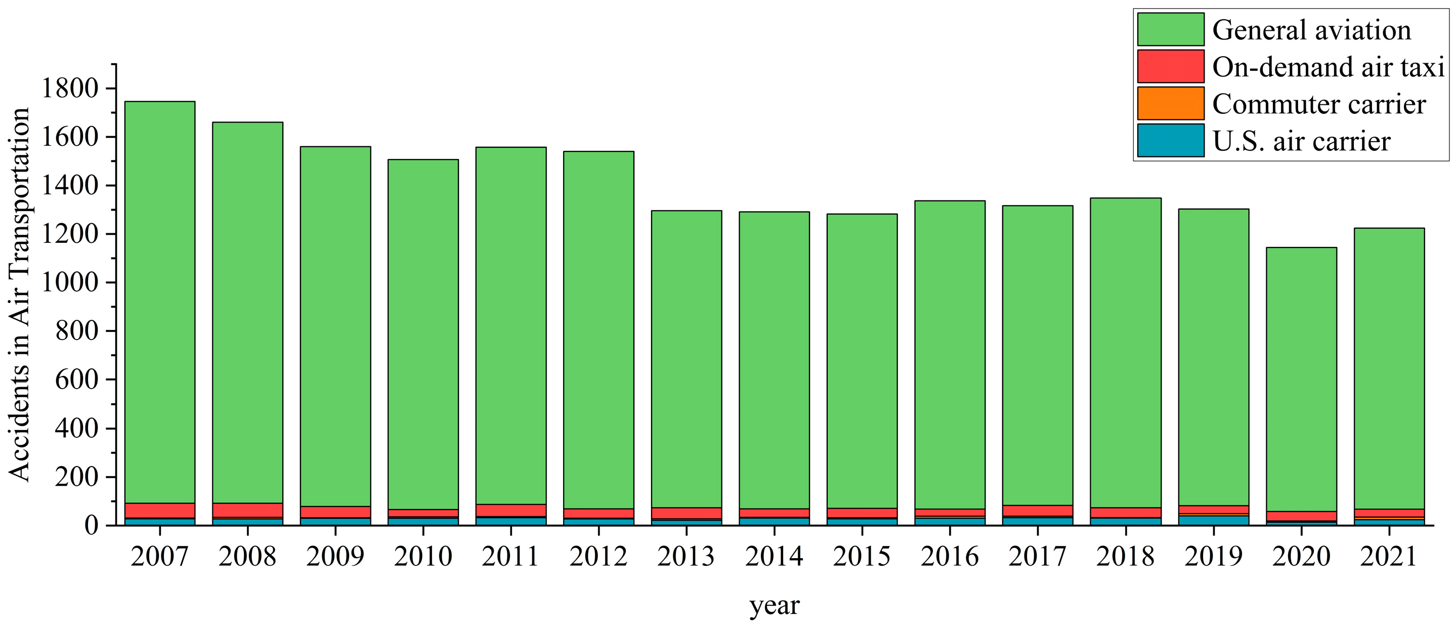
The rest of the paper is organized as follows: Section 2 briefly introduces the source of the data and the construction of multi-timescale series. Section 3 discusses seasonal time series decomposition, the theory of nonlinear chaotic characteristic determinations, and the CSSA-LSSVM forecasting model. Section 4 analyzes the results of the experiment and the prediction simulation findings. Finally, Section 5 summarizes the conclusions of this paper and suggests directions for future research.

2. Data Processing

2.1. Data Sources

The general aviation industry in the United States is huge and diversified, including drones, light aircraft, helicopters, and private jets. Additionally, it has great flexibility and convenience due to the wide variety of flying ranges. However, its huge scale and complexity bring a large number of accidents and huge challenges to safety regulation. According to Transportation Accidents by Mode, published by the United States Bureau of Transportation Statistics, general aviation accidents account for up to 94% of all air transportation accidents from 2007 to 2021. As shown in Figure 1.
The data used in this study comes from the National Transportation Safety Board’s (NTSB) aviation accident database, which records all aviation accidents that have occurred in the United States since 1962. Since the notification of accidents or serious incidents changed in the ninth edition of ICAO Annex 13 [1] in 2001 and considering the impact of the time from the effective date of the document to the time of the accident statistics, when it comes to data records that are 20 years old or older, there are issues with different statistical standards. Additionally, shorter-term data is influenced by specific events, volatility, or random factors. As a result, we studied the preceding 15 years of data based on NTSB statistics, from 2007 to 2021, which can better reflect the current situation and developments, making the study’s findings more relevant. This data contains various types of information, such as accident date, location, aircraft serial number, number of casualties, and so on, which is essential for analyzing general aviation accidents, as shown in Table 1. Our study focused on critical safety risk cycle monitoring. We are interested in how the nonlinear aspect of accident incidence presents itself on time series. We purposefully concentrate on the time series, leaving aside other aspects such as aircraft model, accident location, or reason. As a result, the overall number of accidents and their timing are the main subjects of our study.

2.2. Time Series Construction

Time series [16] analysis facilitates the discovery of hidden information in data and gives insights into the trends, seasonal patterns, and evolutionary processes behind the data, which lead to more accurate predictions of future trends. It is widely used in fields such as military science, economics, meteorology, and medicine for forecasting and decision-making. The purpose of time series analysis is to better understand and predict future trends by modeling the structure of time series data using temporal statistical characteristics. In a review of time series analysis of road safety trends [17], Ruth and Joanna analyze the development of time series modeling techniques and applications in several European countries between 2000 and 2012. The main ones include a comprehensive investigation of the frequency and severity of road accidents; an explanation of the analysis of short/medium-term trends; an evaluation of the efficacy of road safety programs; and a long-term prediction of national road safety indicators. However, one must also consider the drawbacks and limits of time series analysis, which requires large quantities of data to construct effective models that can be mined for trends. The general aviation accident dataset used in our study is adequately sized and contains enough important information that it allows for time series analysis, data mining, and prediction modeling.
In the time series construction procedure, firstly, the general aviation accident data were cleaned by eliminating missing values and unknowns. Then data filtering was used to screen all data associated with general aircraft that satisfied the conditions of Federal Aviation Regulations Part 91. Finally, the general aviation accident data have been collated in chronological order, yielding a total of 18,480 accident records. With days as the unit, HM-scale is the statistics every half month, ET-scale is the statistics every 10 days, and EF-scale is the statistics every 5 days. Different timescales were selected for classification statistics to construct the time series of general aviation accidents:
X H M s c a l e = [ x H M 1 , x H M 2 , ]
X E T s c a l e = [ x E T 1 , x E T 2 , ]
X E F s c a l e = [ x E F 1 , x E F 2 , ]
where XHM-scale, XET-scale, and XEF-scale represent the time series of HM-scale, ET-scale, and EF-scale, respectively.
In this way, the subsequence of American general aviation accidents was constructed as a sample for subsequent multi-timescale series analysis, as shown in Figure 2.

3. Methodology

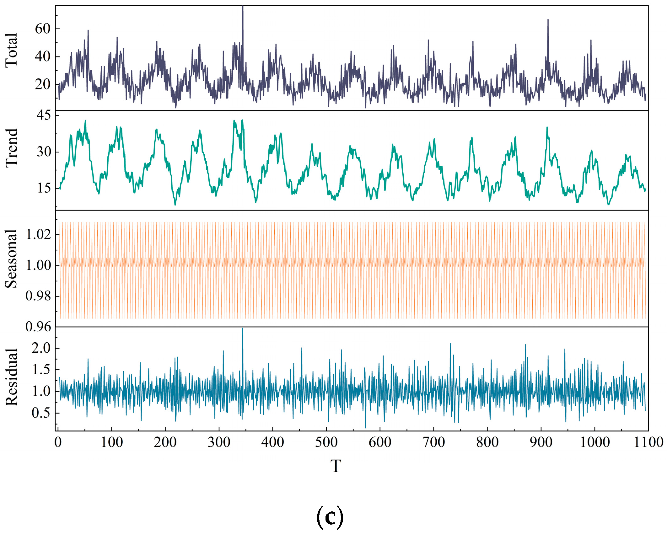
3.1. Time Series Seasonality Decomposition

Since the time distribution of general aviation operation has obvious seasonal regularities, that is, general aviation activities are more frequent in peak seasons, various types of general aviation accidents increase at these times, and general aviation volume and accidents are lower at the beginning and end of each year. To exclude periodic changes in the sequence, seasonal decomposition is performed on the counted time series to better understand the contributions of different components in the sequence and their interactions. Time series seasonal decomposition [16] is the process of decomposing a time series into three parts: trend (T), seasonality (S), and residual (R). The trend is the long-term stable change of the time series, reflecting the overall trend of change in the sequence. Seasonality is a term for periodic short-term fluctuations, usually caused by seasonal factors. Finally, the residual part contains noise or components in the time series that cannot be explained by trend and seasonality. The function can be expressed as:
Y t = f ( T t , S t , R t )
where Tt is a trend over a longer period, called the trend term; St is the change caused by seasonal changes, called the seasonal term; and Rt is the remaining part of the time series caused by numerous chance factors, after separation, called residuals.
Seasonal decomposition is mainly divided into two types: multiplicative model and additive model. For additive models, seasonal components are superimposed on trends and residuals in fixed values, that is:
Y t a d d = T t + S t + R t
For multiplicative models, seasonal components affect the entire time series in relative proportions:
Y t m u l = T t × S t × R t
Therefore, additive models are suitable for situations where the size of seasonal components does not change too much over time, while multiplicative models are suitable for situations where seasonal components change greatly over time, such as historical accident data in general aviation in this study.
After decomposing multi-timescale sub-sequences of general aviation accidents seasonally according to seasonality multiplication method, we obtain the time series of trend, seasonality, and residuals as shown in Figure 3.
Through seasonal decomposition of time series at different scales, it is found that the accidents are more stochastic and exhibit obvious chaotic characteristics, including long-term irregular oscillations and complex fractal structures, under multi-timescale series. Since traditional time series analysis methods cannot model and predict it well, in our study, we use chaos analysis methods to explore the dynamic characteristics and nonlinear behavior of time series of different scales.

3.2. Multi-Timescale Series Nonlinear Analysis

Chaos theory [18] refers to the “intrinsic randomness” in deterministic systems. It is not simply “disorder” or “chaos”, but an “ordered” state with a rich internal hierarchy without obvious periodic changes. It is one of the theories for studying the dynamic behavior of nonlinear systems. The analysis and determination of chaotic characteristics are prerequisites for predicting general aviation accidents. The 0–1 test [19] and the maximum Lyapunov exponent technique are utilized in our study to determine the chaotic characteristics of time series. The following are the steps:
Step 1: Based on the National Transportation Safety Board (NTSB) data statistics, we construct a time series of general aviation accident history data by seasonal decomposition to exclude cyclical patterns X = [x1, x2, …, xN].
Step 2: Use the 0–1 test to verify chaotic characteristics by constructing translation variables p(n) with q(n) and calculating the mean square displacement Mc(n) and its growth rate Kc. When the growth rate Kc approaches 1, it has chaotic characteristics; otherwise, it does not have chaotic characteristics.
Step 3: Using the mutual information approach [20] and the Cao algorithm [21], calculate the delay time τ and embedding dimension m for phase space reconstruction of general aviation accident data series.
Step 4: Recreate the phase space of a general aviation accident time series based on Step 3. X(t) = {x(t), x(t + τ), …, x[t + (m − 1)τ]} is the reconstructed phase space.
Step 5: Using the maximum Lyapunov exponent method, determine the characteristics of the general aviation accident time series. The general aviation accident time series is chaotic when the Lyapunov exponent is larger than zero; otherwise, it is non-chaotic.
The 0–1 test is a chaos detection theory proposed by Melbourne et al. [19] in 2016. Its biggest feature is that it does not require any phase space reconstruction and can directly act on time series to determine its chaotic characteristics. Firstly, two translation variables are defined as p(n) and q(n):
p ( n ) = i = 1 n x ( i ) cos ( θ ( i ) ) , n = 1 , 2 , , L
q ( n ) = i = 1 n x ( i ) sin ( θ ( i ) ) , n = 1 , 2 , , L
where θ(i) = ic + ∑x(k), x(i) are the sequences to be tested, and c ∈ (o,π) is a random constant, generally L = N/10.
If the phase diagram of p(n) with q(n) shows irregular motion characteristics, then there is chaos in the original time series; otherwise, there is none. To study the dispersion characteristics of p(n) with q(n), define mean square displacement Mc(n):
M c ( n ) = lim 1 N i = 1 N { [ p c ( t + n ) p c ( t ) ] 2 + [ q c ( t + n ) q c ( t ) ] 2 }
Define oscillation term:
V O C S ( c , n ) = ( E ( x ) ) 2 1 cos ( n c ) 1 cos ( c )
where  ( E ( x ) ) 2 = lim N 1 N j = 1 N x ( j ) .
After correcting mean square displacement, good convergence characteristics will be obtained. The corrected mean square displacement is:
D c ( n ) = M c ( n ) V O C S ( c , n )
where Mc(n) and Dc(n) have the same asymptotic linear growth rate, but Dc(n) converges better. When the phase diagram of p(n) with q(n) shows irregular motion, i.e., Brownian motion characteristics, Mc(n) increases linearly with time. Calculate asymptotic growth rate Kc:
K c = lim n log D c ( n ) / n
If Kc ≈ 1, the time series has chaotic characteristics; if Kc ≈ 0, the time series does not have chaotic characteristics.
Phase space [22] is a multi-dimensional space describing the evolution of a set of physical quantities. In chaotic systems, evolution trajectories between different states may intersect and overlap. To solve this problem, phase space reconstruction is applied, which involves mapping time series into high-dimensional space using procedures such as sampling and delay embedding so that neighboring states have obvious distance correlations in phase space.
According to Takens [23], the theory proves that if the embedding dimension is large enough to recover the dynamical properties of the system with topological equivalence, the reconstructed phase space can retain many properties of the dynamical system, allowing the prediction of chaotic time series. Determining delay time τ and embedding dimension m are critical steps in the phase space reconstruction process. There are many studies on selecting relevant parameters. Among them, the mutual information method can well measure nonlinear correlation between time series, so it is widely used to obtain optimal delay time.
Suppose general aviation accident time series is {xi|i = 1, 2, …, n}, residual time series is {yj|j = 1, 2, …, n}, assuming xi and yj probability density are Px(xi) and Py(yj), respectively, their joint density is Pxy(xi, yj), and set delay time as τ, then the mutual information function is:
I ( τ ) = i = 1 i + τ P x y [ x i , x i + τ ] ln P x y [ x i , x i + τ ] i P x ( x i ) ln P x ( x i ) i + τ P y ( x i + τ ) ln P y ( x i + τ )
Let τ increase from small to large calculate I(τ), take corresponding when first minimum value appears as optimal delay time τ.
Among methods for calculating embedding dimension, the Cao method improves on pseudo-nearest neighbor method reconstructs dimensional phase space:
X ( t ) = { x ( t ) , x ( t + τ ) , , x [ t + ( m 1 ) τ ] }
a ( i , m ) = X i ( m + 1 ) X n ( i , m ) ( m + 1 ) X i ( m ) X n ( i , m ) ( m ) , i = 1 , 2 , , N m τ
where ‖∙‖ is the Euclidean distance; Xi(m) and Xi(i,m)(m) are the ith vector in m dimensional space and its nearest neighbors; Xi(m + 1) and Xi(i,m)(m + 1) are the ith vector in m + 1 dimensions and its nearest neighbor; n(i, m) is an integer greater than or equal to 1 and less than N.
Calculate average for all a (i, m) get:
E ( m ) = 1 N m τ i = 1 N m τ a ( i , m )
Define change from m dimension to m + 1 dimension as:
F ( m ) = E ( m + 1 ) E ( m )
Through calculating the time delay τ between time series data, in the reconstructed phase space, the value of m corresponding to when F(m) tends to be stable is the minimum embedding dimension.
The Lyapunov exponent is an important physical quantity used to identify a system’s chaotic state, assess the degree of chaos, and define the system’s sensitivity to tiny perturbations. It can be estimated using the system’s evolution rate and the distance change rate after phase space reconstruction [24]. The commonly used calculation methods include the Jacobian method and Wolf method [25]. The small data volume method, which is computationally simple and dependable, is applied in this study. After phase space reconstruction, the nearest neighbor point Xj of each reference point Xi is found, and its distance is dM(0):
d M ( 0 ) = min X i X j , | i j | > p
where p is average period series.
The estimation formula of maximum Lyapunov exponent is
λ 1 ( i ) = 1 i Δ t 1 M k i = 0 M k ln d t ( i ) d t ( 0 )
where ∆t is sample period and di(i) is distance between t pair of nearest points after i discrete steps.
For ∀i calculate take logarithm of above formula get
ln d t ( i ) = ln C t + λ i ( i Δ t ) , t = 1 , 2 , , N
where Ct = dt(0) is constant.
The maximum Lyapunov exponent can be considered as the slope of the above set of straight lines, which can be obtained by least squares approximation of this set of straight lines, i.e.,
y ( i ) = 1 q Δ t j = 1 q ln d j ( i )

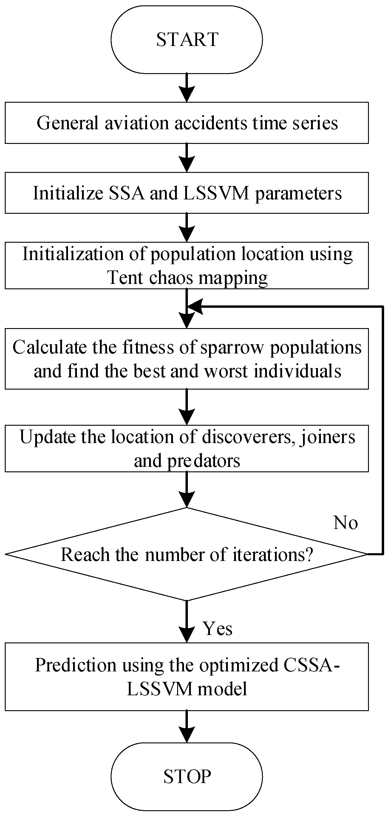
3.3. Multi-Timescale Series Prediction Model

A time series is a collection of data used to describe changes in one or more characteristics over time. The analysis of time series is a statistical analysis method for modeling and forecasting time series data that aims to uncover intrinsic patterns and trends from past observations and use historical data to predict trends and changes in the future.
Analyzing and modeling historical data is the initial stage in time series prediction. The two primary groups of prediction techniques are statistical methods and machine learning methods. The most common statistical methods are: Moving Average model (MA), Exponential Smoothing model (ES), Autoregressive Integrated Moving Average model (ARIMA), Seasonal Autoregressive Integrated Moving Average model (SARIMA), Holt–Winters model, and Vector Autoregressive model (VAR). Among them, MA, and ES [26] are usually used for short-term forecasting problems. ARIMA [27] and SARIMA [28] can be applied to a wide range of time series data. VAR [29] is usually used for multivariate time series data. These statistical methods have shown that the prediction results were not appropriate in subsequent experiments.
Compared with traditional statistical methods mentioned above, methods based on machine learning have advantages such as self-learning, adaptability, and good fault tolerance. They can handle complex nonlinear problems well and have been widely used in fields such as nonlinear time series prediction. The major machine learning-based methods are Support Vector Machine (SVM) and Deep Learning models including Convolutional Neural Network (CNN), Artificial Neural Networks (ANN), Recurrent Neural Network (RNN), and Long Short-Term Memory Network (LSTM) models. These methods can handle nonlinear relationships and long-term dependencies, and usually perform well with large amounts of data. For time series prediction problems, SVM [30] can be used to solve classification and regression problems and to predict future data points. CNN [31] can be used to extract local correlations in time series data. ANN [32] can be used to capture long-term dependencies in time series data. LSTM [33] can be used to handle complex time series data.
However, the drawback of machine learning algorithms for prediction is that the parameters utilized have a large influence on the prediction results. A model that is too complicated or flexible can lead to overfitting, which occurs when the model performs well on training data but poorly on test data. On the other hand, a model that is too simple can lead to underfitting. The purpose of intelligent algorithm optimization (e.g., GA [34], PSO, and SSA [35]) is to prevent parameter uncertainty from influencing prediction results.
The Least Squares Support Vector Machine (LSSVM) [36] is an improved support vector machine based on statistical theory that can transform the solution of a quadratic optimization problem into the solution of a system of linear equations. Thus, it simplifies the solution of the problem, is very effective in dealing with nonlinear data, and has a high prediction accuracy. The training process of LSSVM involves only a small number of support vectors, so it can efficiently handle large-scale datasets. We utilize the general aviation accident data set over the last 15 years and account for the number of accidents based on the time series. There are 366 (for the HM-scale), 548 (for the ET-scale), and 1096 (for the EF-scale) sample points available for prediction. Yu et al. [37] applied RBD-LSSVM for time series prediction with 279 samples for yearly prediction and 522 samples for monthly prediction. In addition, Sun et al. [38] suggested the VMD-P-(ARIMA, BP)-PSOLSSVM model, which employed 1000 samples of wind speed data as projections, and they both developed optimized prediction results. After the LSSVM training process, the final decision function consists of only a small number of support vectors. In our experiment, 8–25 support vectors are used to process the data set efficiently and accurately. The disadvantage is that the parameters can easily influence the predictions. Therefore, our study is based on the LSSVM model and proposes a chaotic mapping sparrow search technique [39] to optimize the parameters, and it creates a CSSA-LSSVM augmented time series prediction model to predict general aviation accident time series.
With good generalization performance and robustness to noise and outliers, the LSSVM is implemented as follows:
Set the input and output of the training set as (xi, yi), i = 1, 2, …, N, and construct the regression estimation function:
f ( x ) = ω T φ ( x ) + b
where ω is the weight vector, φ(x) is the nonlinear mapping function, and b is the bias term.
By optimizing the regression error parameter to minimize cost, construct the objective function:
min W = 1 2 ω T ω + C i = 1 N e i 2
s . t . ω T φ ( x ) + b = 1 e i
where C is the regularization function and ei is the prediction error of the ith sample.
This objective function is a quadratic programming problem with constraints that can be solved using Lagrange multipliers.
L ( ω , b , e , a ) = 1 2 ω T ω + C i = 1 N e i 2 i = 1 N a i [ ω T φ ( x ) + b + e y i ]
where ai are Lagrange multipliers. Taking partial derivatives of each variable in the above formula yields:
{ L ω = 0 ω = i = 1 N a i φ ( x i ) L b = 0 i = 1 N a i = 0 L e i = 0 a i = c e i L a i = 0 ω T φ ( x i ) + b + e i y i = 0
By solving the above equation, the LSSVM regression function can be obtained as
f ( x ) = i = 1 N a i K ( x , x i ) + b
where K(x,xi) is the kernel function.
Common kernel functions [40] include linear kernel functions, Sigmoid function, polynomial kernel functions, radial basis function (RBF), etc. RBF is frequently employed in many practical situations because it can map nonlinear data into high-dimensional space and make it linearly separable in high-dimensional space. Compared with polynomial kernel functions, RBF kernel functions require fewer parameters and are suitable for handling nonlinearly differentiable data. As the parameter σ increases, it has a wider range of influence on the training set, which leads to a more relaxed decision boundary and increases the generalization ability of the model.
Its expression is:
K ( x , x i ) = exp ( x x i 2 2 σ 2 )
where‖∙‖ is the Euclidean distance, xi is the specified center point, and σ is a parameter representing the width of the kernel function from the center point. The smaller the value, the wider the range of action, and vice versa.
A unique swarm intelligence technique, initially proposed by Xue et al. [41] in 2020, replicates the interaction behavior of a bunch of sparrows during the food hunt process. Using this behavior, the answer to the problem is eventually optimized through continual exploration and learning.
The core idea of SSA is to regard the search space as an ecosystem. Where each individual represents a solution, and the total population corresponds to the set of all viable solutions. Individual sparrows compete with one another in this ecosystem, sharing knowledge and adapting to the environment to find the optimal answer.
Individuals in SSA are divided into three groups: discoverers, joiners, and predators. Among them, discoverers are individuals with strong exploratory and innovative abilities who randomly search for new position vectors and pass on all solutions obtained during the search to other individuals. The joiners learn and evolve by learning from the experience of the surrounding individuals to improve their own position vectors. Predators, on the other hand, have a strong competitive ability, and they choose the position vector of the individual with the highest fitness value in the neighborhood range to update. The specific rules are as follows:
  • Initialize population:
Randomly generate initial solutions according to the dimension and number of individuals in the search space. Assume there are N sparrow groups in a D-dimensional search space. The ith sparrow’s position in the search space can be expressed as
Z i = [ z i 1 , , z i d , , z i D ]
where zid is the position of the ith discoverer in the dth dimension.
2.
Discoverer explores new solutions:
The discoverer explores continually and at random for better solutions. Specifically, in each iteration, the new location of each individual discoverer is calculated using the following equation:
z i j ( t + 1 ) = { z i j ( t ) exp ( i α i max ) , R 2 < S T z i j ( t ) + Q L     R 2 S T
where j = 1, 2, …, d, t is current iteration times; zij(t) is the position of ith discoverer in jth dimension; α is a uniform random number between [0, 1]; Q is a random number of normal distributions; imax is the maximum number of iterations; and L is a 1 × d dimensional matrix with all elements equal to 1:
When R2 < ST, it means that environment is safe at this time and discoverer will forage here; when R2ST, it means that current environment is dangerous at this time sparrow goes to safe area for foraging.
3.
Joiner updates position:
Joiners receive new solutions provided by discoverers, compare them with their own existing solutions, and update their own positions with better solutions. Specifically, in each iteration, for each joiner individual, calculate its new position according to the following formula:
z i j ( t + 1 ) = { Q exp ( z w o r s t ( t ) z i j ( t ) i 2 ) ,   i > n 2 z P ( t + 1 ) + | z i j ( t ) z P ( t + 1 ) |   A + L i n 2
where zp(t) and zworst(t) are respectively represent current optimal position and global worst position occupied by discoverer; A is a 1 × d dimensional matrix whose elements are randomly assigned 1 or −1; and A+ = AT(AAT)−1.
4.
Predator updates position
Predators improve their positions through interaction with other individuals in the population, gradually occupying dominant positions. Specifically, in each iteration select part of individuals as predators and calculate their new positions according to the following formula:
z i j ( t + 1 ) = { z b e s t ( t ) + β | z i j ( t ) + z b e s t ( t ) | , f i > f g z i j ( t ) + λ   ( | z i j ( t ) z w o r s t ( t ) | ( f i f w ) + ε ) ,     f i = f g
where zbest(t) is the global optimal position of population at tth iteration; β is a random number following standard normal distribution; λ is a random number following uniform distribution in [−1, 1] interval; ε is a very small constant adding is to prevent occurrence of denominator fgfw = 0; fi is current individual fitness; fg is global optimal fitness; and fw is global worst fitness.
When fi > fg, it means that the sparrow is at the edge of the population and vulnerable to attack; when fi = fg, it means that the sparrow has discovered danger and needs to move foraging location.
Since the standard sparrow search algorithm suffers from the lack of population diversity and the position update result depends on the initial position of the population during the iterative process, when exploring the solution space, it is easy to fall into the local optimal solution, and it cannot guarantee finding the global optimal solution. In contrast, chaotic mapping is a nonlinear dynamical system with a stochastic nature, which can generate a large number of sequences of random numbers. Chaotic Sparrow Search Algorithm (CSSA), by introducing the Tent chaotic mapping into the sparrow search algorithm, can increase the stochasticity in the algorithm. Thus, it helps to avoid the situation of falling into local optimal solutions and improves the global optimization capability of the algorithm [42]. The Tent mapping is defined as follows:
y i + 1 = { 2 y i , 0 y < 0.5 2 ( 1 y i ) , 0.5 y 1
Through Bernoulli transformation, get the formula
y i + 1 = ( 2 y i ) mod 1
where yi is before the chaotic mapping and yi+1 is after the chaotic mapping.
The detailed flow of the time series prediction model of general aviation insecurity events based on CSSA-LSSVM is shown in Figure 4.
The specific steps are:
Step 1: Create a time series of general aviation accidents and determine the number of training and test samples.
Step 2: Initialize the SSA and LSSVM model parameters, including the population size, the proportion of discoverers to the population, the maximum number of iterations, etc.
Step 3: Initialize the population location distribution using Tent chaos mapping.
Step 4: Calculate the initial fitness fi of each sparrow and find the best and worst individuals.
Step 5: Update positions of discoverer, joiner, and predator sparrows in sparrow population, according to Formulas (30)~(32) calculate fitness of new position of sparrows, and update fg and fw.
Step 6: Determine whether stopping condition is reached; if so, output global optimal parameters, otherwise go to step 4.
Step 7: Obtain an optimal prediction model and do prediction simulation experiments.

4. Simulation Analysis

4.1. Multi-Timescale Series Nonlinearity Validation

Time series chaos analysis is a common method used to study the behavior of nonlinear dynamic systems. In our paper, the 0–1 test of chaos identification is used to distinguish chaotic signals from random noise by determining whether the time series satisfy the random property. For the multi-timescale sequence of general aviation accidents, the HM-scale time series is analyzed as an example, and the phase diagram of p(n) with q(n), as shown in Figure 5, and the change graph of Mc(n) and Dc(n) with time, as shown in Figure 6.
We can find that the dispersion characteristics of the phase diagram of p(n) with q(n) conform to Brownian motion, and Mc(n) and Dc(n) both increase linearly with time. The asymptotic growth rate is Kc = 0.9981, that is Kc→1, so the HM-scale series has chaotic characteristics.
Moreover, the phase diagrams of ET-scale and HM-scale, as shown in Figure 7 and Figure 8, are still consistent with the Brownian motion stochastic characteristics, and the asymptotic growth rate Kc both tend to 1. As such, the general aviation accident multi-timescale series have chaotic characteristics.
The phase space reconstruction is performed by calculating the embedding dimension m and the delay time τ, and the Lyapunov exponent is calculated to determine the chaotic properties of the time series. The iy(i) function is displayed using multi-timescale data. In addition, after fitting with the least squares approach, the slope of the line equals the time series’ maximum Lyapunov exponent, as shown in Figure 9.
The maximum Lyapunov exponents of time series at multi-timescales are all positive, proving that general aviation accident time series exhibit chaotic properties. The high complexity and irregular characteristics exhibited by the time series of general aviation accidents come from their inherent nonlinear dynamic system, which makes them very sensitive to small changes in initial value conditions. Although the complexity of time series and extreme sensitivity to initial values make it difficult to predict their future accurately, short-term prediction is possible. The use of time series analysis techniques can help identify these patterns and trends and predict future trends.

4.2. Multi-Timescale Series Predicting Simulation Analysis

In our study, we utilize the modified Chaotic Sparrow Search Algorithm (CSSA) to optimize the parameters of LSSVM. The CSSA-LSSVM model is established and verified through simulation. Set the parameters of CSSA-LSSVM: population size NP = 5, number of iterations T = 100, parameters ST = 0.8, and discoverer ratio of 0.2. Taking the general aviation accident series data set as an example, 80% of the data in the time series is used for training, and the remaining 20% of the data is used to form a test set to simulate and predict multi-timescale series experiments. The results show that after 3–5 iterations of the heuristic method, the model could reach stability, and the prediction effect is good, as shown in Figure 10. This indicates that the improved sparrow search method has a promising future to optimize SVM parameters. As illustrated in Figure 11, the predicted outcomes are compared to the real numbers.
Take the HM-scale as an example to demonstrate the effectiveness and superiority of the CSSA-LSSVM prediction model. The model proposed in our study is compared with the models optimized by other intelligent algorithms (including: SSA-LSSVM, GA-LSSVM, PSO-LSSVM) and the conventional time series prediction models (including LSSVM, CNN, ANN, LSTM, ARIMA, and Holt–Winters models). The prediction results are shown in Table 2. When calculating the error analysis, the normalization step is omitted to save time and complexity since the data have the same magnitude and are all in the same magnitude range between 0 and 150.
To compare the prediction impacts of the models, the Root Mean Square Error (RMSE), Mean Absolute Error (MAE), and correlation coefficient (R2) metrics were determined. The CSSA-LSSVM model developed in this study is found to be closer to the real data than other models, and its prediction performance is greatly enhanced. It achieves state-of-the-art results in the field of general aviation accident time series prediction in the dataset utilized in our research.
By comparing the prediction of time series at different scales, it is found that the prediction error gradually decreases as the timescale granularity decreases, but the fitting effect of the prediction results shows a tendency to initially grow and then reduce. Specifically, when the time granularity decreases to a certain degree, the fitting effect of the prediction results becomes better and the R2 value increases. However, when the time granularity continues to decrease, the fitting effect of the prediction results decreases, and the R2 value decreases. The calculation results are shown in Table 3.
This experimental conclusion indicates that the model may have overfitting problems on the training data, and it is important to choose the appropriate time granularity in the prediction process. In the prediction of large-scale time granularity (HM-scale in our study), it frequently faces the problem of insufficient peak prediction and produces undesirable outcomes. In their investigation of the fluctuation of flight flow, Zhang et al. [43] shown that the long time granularity is not particularly important for prediction due to the effect of chaotic characteristics. In contrast, there is insufficient sensitivity to quick fluctuation situations in the prediction of small-scale time granularity (EF-scale in our study), resulting in lower prediction accuracy. Yu et al. [7] demonstrated in their study of chaos analysis and prediction of airplane accidents that the smallest time granularity does not guarantee the best prediction results. However, at intermediate scales, the prediction model is able to better balance these two aspects, improving the accuracy of the predictions. In the experiments of this study, the fitting accuracy is better at the ET scale, which can well reflect the nonlinear characteristics of the time series of general aviation accident.

5. Conclusions

To better understand the characteristics of general aviation accidents, our study analyzes multi-timescale historical statistics of general aviation accidents. On the basis of machine learning, a chaotic sparrow search Least Squares Support Vector Machine prediction model is suggested. The main conclusions of our research are as follows:
(1)
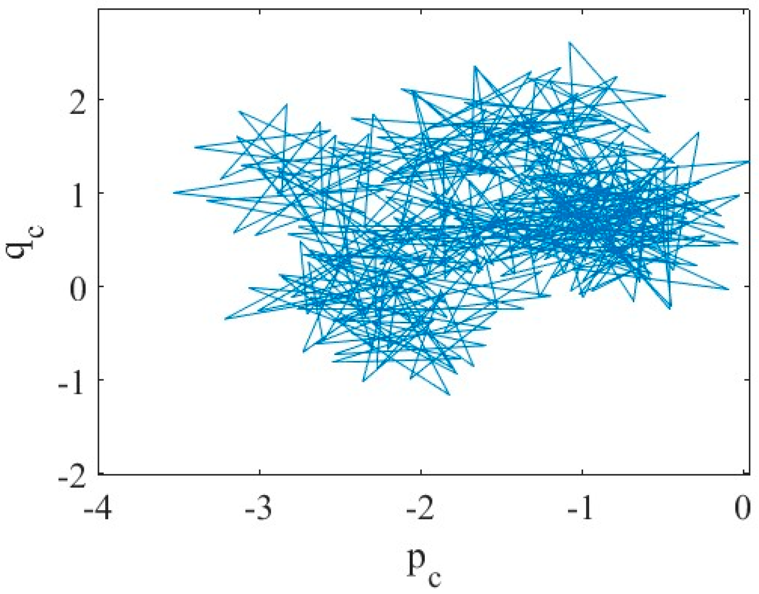
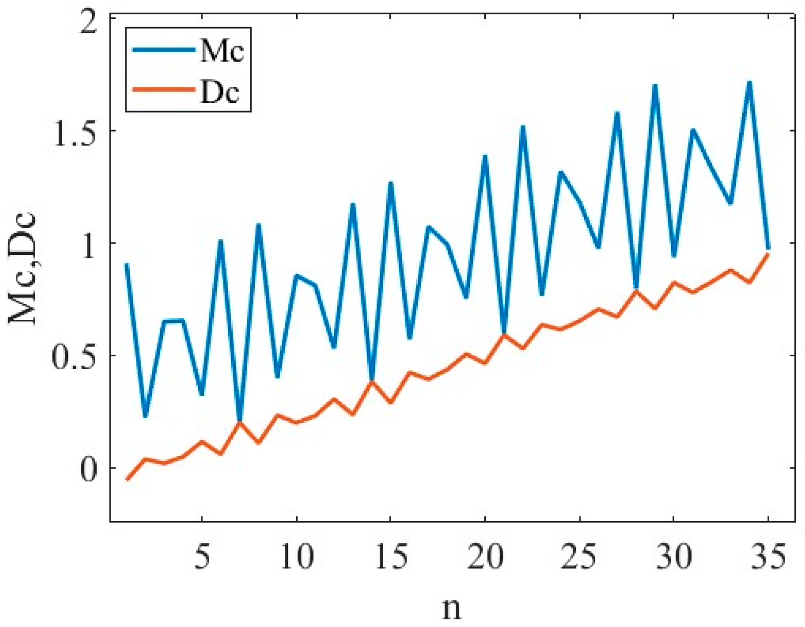
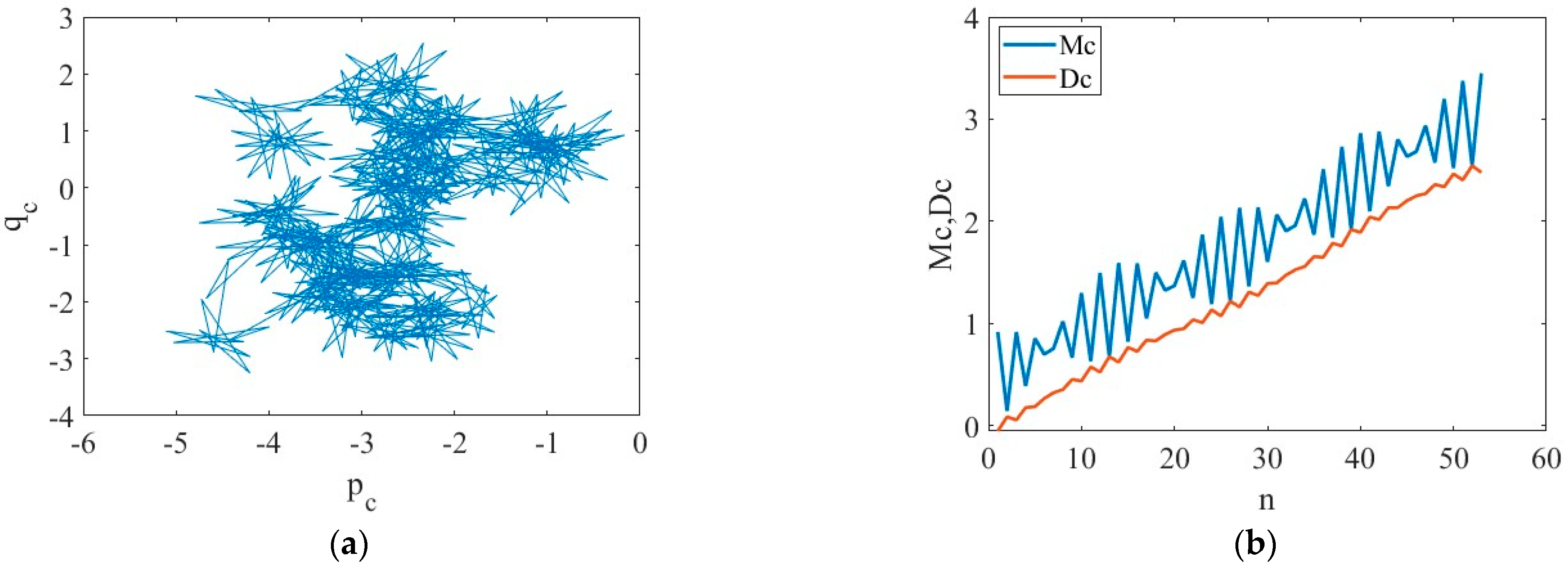
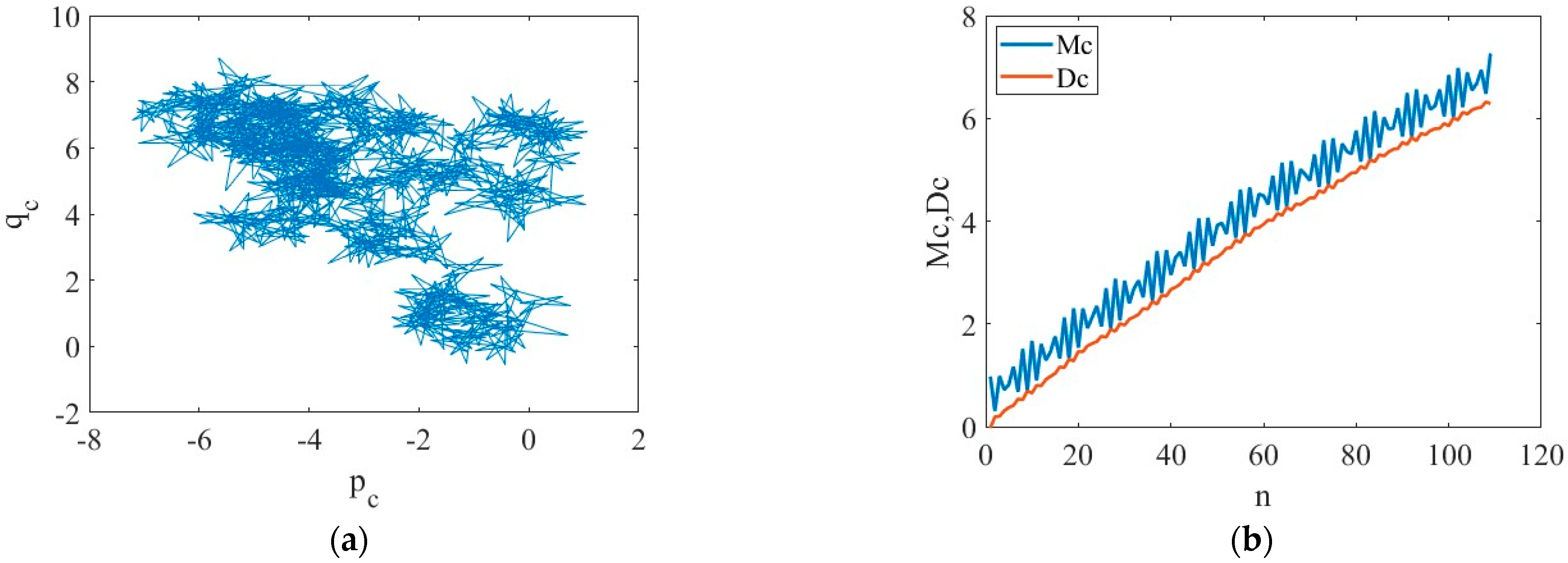
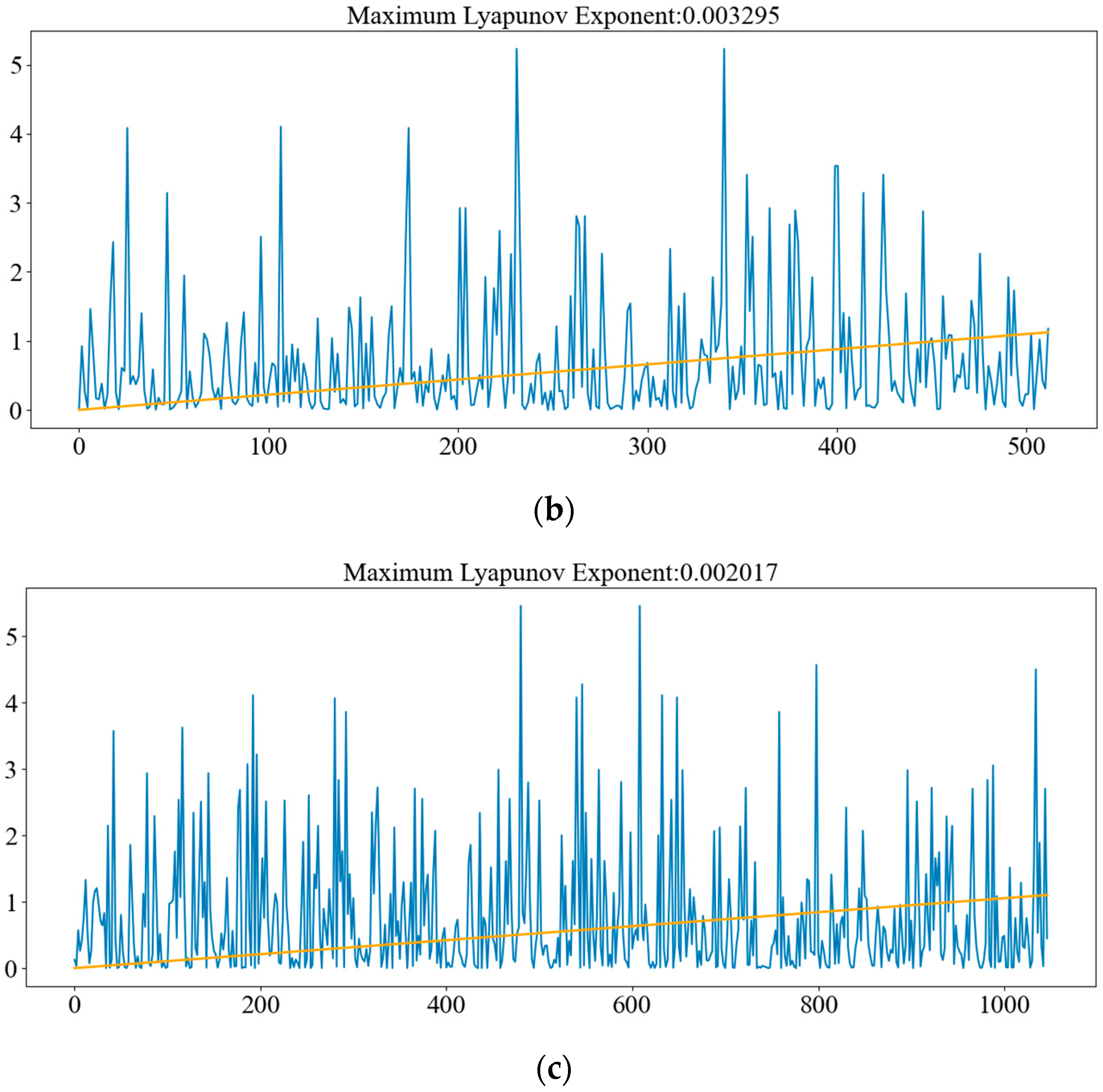
The residual parts of the decomposition show the apparent randomness and irregular oscillations of the general aviation accident time series. As a consequence, the nonlinear characteristics of the time series have been investigated in this study. The 0–1 test shows that the phase diagram possesses Brownian motion features, and the Lyapunov exponent is positive at all three timescales. Both prove that the multi-timescale series of general aviation accidents show a chaotic pattern. With a decreasing timescale, there is no substantial change in time delay, embedding size, or maximum Lyapunov exponent.
(2)
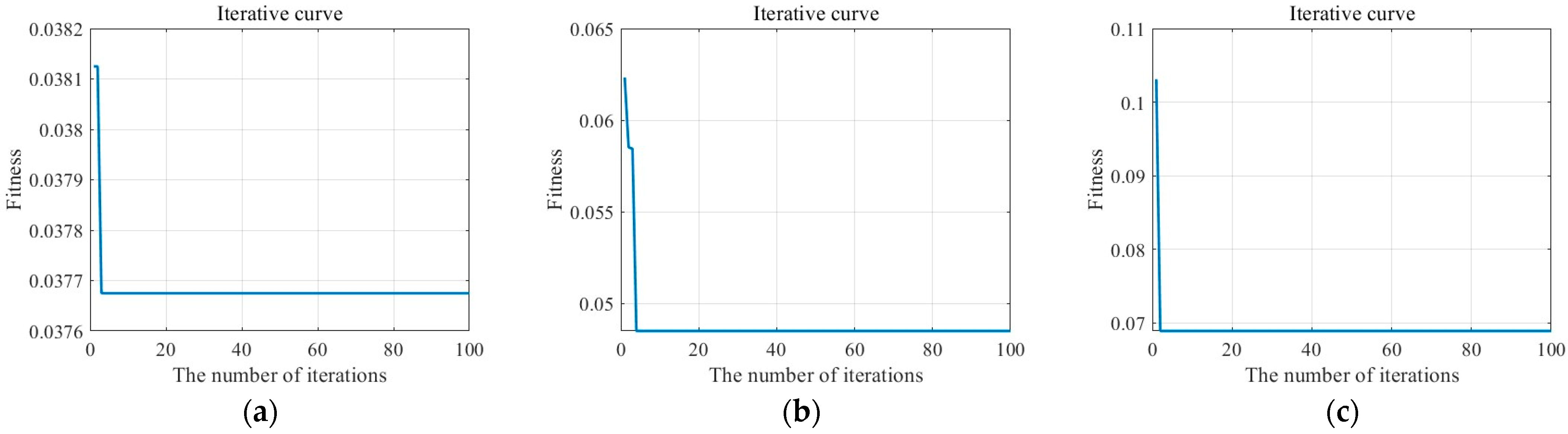
The parameters of the LSSVM model are optimized by the chaotic sparrow search algorithm, and the prediction method of the CSSA-LSSVM model is proposed. The experimental simulation prediction effect is quantified and analyzed with the root mean square error (RMSE), mean absolute error (MAE), and correlation coefficient (R2). Compared with the original LSSVM model, the proposed CSSA-LSSVM model has obvious advantages and shows higher prediction results in simulation experiments. The accuracy of RMSE, MAE, and R2 is significantly improved in these three performance evaluations.
(3)
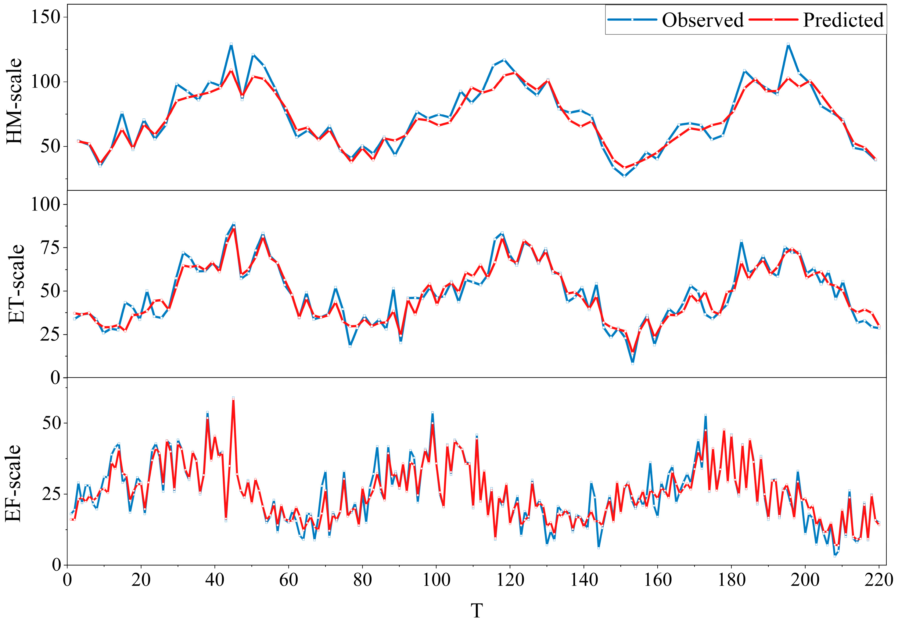
By comparing with other conventional time series prediction algorithms, the CSSA-LSSVM model is superior to them in terms of lesser errors, faster iterative convergence, and better fit. In addition, by comparing the prediction effect over different timescales, the prediction error is shown to be lower at a smaller timescale (EF-scale), showing that dividing the general aviation accident time series into fine-grained subseries benefits accurate prediction. While the timescale with the most accurate fit is ET-scale, indicating that the smallest granularity is not the best, the performance of multiple granularities must be examined to discover the optimal value.
In conclusion, the research conducted in our study on the multi-timescale series of general aviation accidents demonstrates the inherent chaotic characteristics of the accident time series. This provides tools for time series analysis of general aviation accidents, which may be utilized for predicting general aviation accidents in the short term and serve as a reference for general aviation safety situational awareness and monitoring. The chaotic characteristics of accidents can help us better comprehend the time series patterns of accident occurrence. This helps practitioners in the industry grasp the complexities and suddenness of accidents. It also helps in the selection of a suitable temporal granularity for future time series prediction. Practitioners in the industry can identify risks and trends from the beginning by analyzing the multi-timescale series of general aviation accidents. It gives vital information for accident prevention, allowing practitioners to take appropriate steps to mitigate the possibility of accidents as soon as feasible and construct more accurate and effective security procedures, consequently improving overall safety. Studies on accident time series prediction help identify risk patterns and periods of time. They can be used as a reference for time series accident monitoring to offer early warning of significant risk periods. In the future, studies could possibly subdivide distinct types of accidents, improve prediction results, and provide theoretical guidelines for general aviation safety risk management.

Author Contributions

Conceptualization, Y.W. and H.Z.; methodology, Y.W. and Z.S.; software, H.Z. and Z.S.; validation, Y.W., Z.S. and W.L.; formal analysis, Z.S. and J.Z.; investigation, Y.W. and W.L.; resources, Z.S.; data curation, W.L.; writing—original draft preparation, Y.W., W.L. and Z.S.; writing—review and editing, Y.W., Z.S., J.Z. and H.Z.; visualization, Y.W. and Z.S.; supervision, H.Z. All authors have read and agreed to the published version of the manuscript.

Funding

This research is funded by National Natural Science Foundation of China: Research on Key Technologies of Multi-scale Intelligent Situational Awareness for Air Traffic Control Operation Safety in Civil Aviation [U2133207]. Research on Aircraft Autonomic Operation Technology by Air-Ground Information Synergetic Sharing [MJZ1-7N22].

Institutional Review Board Statement

Not applicable.

Informed Consent Statement

Not applicable.

Data Availability Statement

The data used and processed during the current study are available from the corresponding author on request.

Conflicts of Interest

The authors declare no conflict of interest.

References

  1. ICAO. ICAO Annex 13 to the Convention on International Civil Aviation: Aircraft Accident and Incident Investigation; ICAO: Montreal, QC, Canada, 2010. [Google Scholar]
  2. He, P.; Sun, R. Research on Cross-Correlation, Co-Integration, and Causality Relationship between Civil Aviation Incident and Airline Capacity in China. Sustainability 2022, 14, 4999. [Google Scholar] [CrossRef]
  3. Bao, J.; Chen, Y.; Yin, J.; Chen, X.; Zhu, D. Exploring Topics and Trends in Chinese ATC Incident Reports Using a Domain-Knowledge Driven Topic Model. J. Air Transp. Manag. 2023, 108, 102374. [Google Scholar] [CrossRef]
  4. Kuhn, K.D. Using Structural Topic Modeling to Identify Latent Topics and Trends in Aviation Incident Reports. Transp. Res. Part C Emerg. Technol. 2018, 87, 105–122. [Google Scholar] [CrossRef]
  5. Arnaldo Valdés, R.M.; Gómez Comendador, V.F.; Perez Sanz, L.; Rodriguez Sanz, A. Prediction of Aircraft Safety Incidents Using Bayesian Inference and Hierarchical Structures. Saf. Sci. 2018, 104, 216–230. [Google Scholar] [CrossRef]
  6. Wang, Y.; Guo, J.; Sun, Y.; Li, C.; Dong, Z. Adaptive Flight Accident Prediction Method Based on Volterra Series. Fire Control Command Control 2020, 45, 115–119. [Google Scholar] [CrossRef]
  7. Yu, H.; Li, X. On the Chaos Analysis and Prediction of Aircraft Accidents Based on Multi-Timescales. Phys. Stat. Mech. Its Appl. 2019, 534, 120828. [Google Scholar] [CrossRef]
  8. Ni, X.; Wang, H.; Che, C.; Hong, J.; Sun, Z. Civil Aviation Safety Evaluation Based on Deep Belief Network and Principal Component Analysis. Saf. Sci. 2019, 112, 90–95. [Google Scholar] [CrossRef]
  9. Zeng, J.; Li, X. Prediction of Mine Subsidence Area Based on Chaotic Time Series Analysis. Gold Sci. Technol. 2019, 27, 249. [Google Scholar]
  10. Meng, Y.; Xu, L.; Yang, J. Application of Multi-Scale Chaotic Time Series Prediction in Early Warning of Electric Equipment Current-Carrying Fault. Dianji Yu Kongzhi Xuebao Electric Mach. Control 2015, 19, 1–7. [Google Scholar] [CrossRef]
  11. Ales, S.; Nico, P.; Paolo, P. Chaos based portfolio selection: A nonlinear dynamics approach. Expert Syst. Appl. 2022, 188, 116055. [Google Scholar] [CrossRef]
  12. Yuan, P.; Lin, X. How Long Will the Traffic Flow Time Series Keep Efficacious to Forecast the Future? Phys. Stat. Mech. Its Appl. 2017, 467, 419–431. [Google Scholar] [CrossRef]
  13. Wang, L.; Zhao, Y. A Method for Predicting Air Traffic Flow Based on a Combined GA, RBF, and Improved Cao Method. J. Transp. Inf. Saf. 2023, 41, 115–123. [Google Scholar] [CrossRef]
  14. Li, G.; Guo, M.; Zhang, H.; Luo, Y. Traffic Status Prediction Method of Regional Air Route Network Based on Chaos Theory. Aeronaut. Comput. Tech. 2020, 50, 61–66. [Google Scholar]
  15. Cheng, A.; Jiang, X.; Li, Y.; Zhang, C.; Zhu, H. Multiple Sources and Multiple Measures Based Traffic Flow Prediction Using the Chaos Theory and Support Vector Regression Method. Phys. Stat. Mech. Its Appl. 2017, 466, 422–434. [Google Scholar] [CrossRef]
  16. Hamilton, J.D. Time Series Analysis; Princeton University Press: Princeton, NJ, USA, 1994. [Google Scholar] [CrossRef]
  17. Bergel-Hayat, R.; Zukowska, J. Road Safety Trends at National Level in Europe: A Review of Time-Series Analysis Performed during the Period 2000–2012. Transp. Rev. 2015, 35, 650–671. [Google Scholar] [CrossRef]
  18. Gaspard, P. Dynamical systems and their linear stability. In Chaos, Scattering and Statistical Mechanics; Cambridge Nonlinear Science Series; Cambridge University Press: Cambridge, UK, 1998; pp. 12–42. [Google Scholar] [CrossRef]
  19. Gottwald, G.A.; Melbourne, I. The 0-1 Test for Chaos: A Review. In Chaos Detection and Predictability; Skokos, C., Gottwald, G.A., Laskar, J., Eds.; Lecture Notes in Physics; Springer: Berlin/Heidelberg, Germany, 2016; Volume 915, pp. 221–247. ISBN 978-3-662-48408-1. [Google Scholar]
  20. Wen, F.; Wan, Q. Time Delay Estimation Based on Mutual Information Estimation. In Proceedings of the 2009 2nd International Congress on Image and Signal Processing, Tianjin, China, 17–19 October 2009; pp. 1–5. [Google Scholar]
  21. Xu, X.; Liu, X.; Chen, X. The Cao Method for Determining the Minimum Embedding Dimension of Sea Clutter. In Proceedings of the 2006 CIE International Conference on Radar, Shanghai, China, 16–19 October 2006; pp. 1–4. [Google Scholar]
  22. Hong, W.C. Phase Space Reconstruction and Recurrence Plot Theory. In Hybrid Intelligent Technologies in Energy Demand Forecasting; Springer: Cham, Switzerland, 2020; pp. 153–179. [Google Scholar] [CrossRef]
  23. Takens, F. Detecting Strange Attractors in Turbulence. In Dynamical Systems and Turbulence, Warwick 1980; Rand, D., Young, L.-S., Eds.; Lecture Notes in Mathematics; Springer: Berlin/Heidelberg, Germany, 1981; Volume 898, pp. 366–381. ISBN 978-3-540-11171-9. [Google Scholar]
  24. Ji, T.; Wang, J.; Li, M.; Wu, Q. Short-Term Wind Power Forecast Based on Chaotic Analysis and Multivariate Phase Space Reconstruction. Energy Convers. Manag. 2022, 254, 115196. [Google Scholar] [CrossRef]
  25. Cencini, M.; Ginelli, F. Lyapunov Analysis: From Dynamical Systems Theory to Applications. J. Phys. Math. Theor. 2013, 46, 250301. [Google Scholar] [CrossRef]
  26. Deng, C.; Zhang, X.; Huang, Y.; Bao, Y. Equipping Seasonal Exponential Smoothing Models with Particle Swarm Optimization Algorithm for Electricity Consumption Forecasting. Energies 2021, 14, 4036. [Google Scholar] [CrossRef]
  27. Xu, D.; Zhang, Q.; Ding, Y.; Zhang, D. Application of a Hybrid ARIMA-LSTM Model Based on the SPEI for Drought Forecasting. Environ. Sci. Pollut. Res. 2022, 29, 4128–4144. [Google Scholar] [CrossRef]
  28. Amshi, A.H.; Prasad, R.; Sharma, B.K. Forecasting Cholera Disease Using SARIMA and LSTM Models with Discrete Wavelet Transform as Feature Selection. IFS 2023, 1–13. [Google Scholar] [CrossRef]
  29. Qian, G.; Tordesillas, A.; Zheng, H. Landslide Forecast by Time Series Modeling and Analysis of High-Dimensional and Non-Stationary Ground Motion Data. Forecasting 2021, 3, 850–867. [Google Scholar] [CrossRef]
  30. Madeira, T.; Melício, R.; Valério, D.; Santos, L. Machine Learning and Natural Language Processing for Prediction of Human Factors in Aviation Incident Reports. Aerospace 2021, 8, 47. [Google Scholar] [CrossRef]
  31. Aryal, S.; Nadarajah, D.; Kasthurirathna, D.; Rupasinghe, L.; Jayawardena, C. Comparative Analysis of the Application of Deep Learning Techniques for Forex Rate Prediction. In Proceedings of the 2019 International Conference on Advancements in Computing (ICAC), Malabe, Sri Lanka, 5–7 December 2019; pp. 329–333. [Google Scholar]
  32. Rafsanjani, M.K.; Samareh, M. Chaotic Time Series Prediction by Artificial Neural Networks. JCM 2016, 16, 599–615. [Google Scholar] [CrossRef]
  33. Lin, L.; Li, M.; Ma, L.; Nazari, M.; Mahdavi, S.; Yunianta, A. Using Fuzzy Uncertainty Quantization and Hybrid RNN-LSTM Deep Learning Model for Wind Turbine Power. IEEE Trans. Ind. Appl. 2020, 1. [Google Scholar] [CrossRef]
  34. Liu, Y.; Du, R.; Niu, D. Forecast of Coal Demand in Shanxi Province Based on GA—LSSVM under Multiple Scenarios. Energies 2022, 15, 6475. [Google Scholar] [CrossRef]
  35. Guo, Z.; Hu, L.; Wang, J.; Hou, M. Short-Term Load Forecasting Based on SSA-LSSVM Model. In Proceedings of the 2021 4th International Conference on Energy, Electrical and Power Engineering (CEEPE), Chongqing, China, 23–25 April 2021; pp. 1215–1219. [Google Scholar]
  36. Tan, G.; Yan, J.; Gao, C.; Yang, S. Prediction of Water Quality Time Series Data Based on Least Squares Support Vector Machine. Procedia Eng. 2012, 31, 1194–1199. [Google Scholar] [CrossRef]
  37. Yu, Y.; Li, J. Residuals-Based Deep Least Square Support Vector Machine with Redundancy Test Based Model Selection to Predict Time Series. Tsinghua Sci. Technol. 2019, 24, 706–715. [Google Scholar] [CrossRef]
  38. Sun, W.; Gao, Q. Short-Term Wind Speed Prediction Based on Variational Mode Decomposition and Linear–Nonlinear Combination Optimization Model. Energies 2019, 12, 2322. [Google Scholar] [CrossRef]
  39. Zhang, C.; Ding, S. A Stochastic Configuration Network Based on Chaotic Sparrow Search Algorithm. Knowl.-Based Syst. 2021, 220, 106924. [Google Scholar] [CrossRef]
  40. Bao, Y.; Wang, T.; Qiu, G. Research on Applicability of SVM Kernel Functions Used in Binary Classification. In Proceedings of the International Conference on Computer Science and Information Technology, Kunming, China, 21–23 September 2013; Patnaik, S., Li, X., Eds.; Advances in Intelligent Systems and Computing. Springer: New Delhi, India, 2014; Volume 255, pp. 833–844. [Google Scholar] [CrossRef]
  41. Xue, J.; Shen, B. A Novel Swarm Intelligence Optimization Approach: Sparrow Search Algorithm. Syst. Sci. Control Eng. 2020, 8, 22–34. [Google Scholar] [CrossRef]
  42. Li, Z.; Luo, X.; Liu, M.; Cao, X.; Du, S.; Sun, H. Wind Power Prediction Based on EEMD-Tent-SSA-LS-SVM. Energy Rep. 2022, 8, 3234–3243. [Google Scholar] [CrossRef]
  43. Xie, Z.; Enyuan, X.; Hongzhi, L.; Yifei, Z.; Mengqi, W. Fluctuation Characteristics of Arrival Flight Flow Based on Limited Penetrable Visibility Graph. J. Transp. Syst. Eng. Inf. Technol. 2022, 6, 244–257. [Google Scholar] [CrossRef]
Figure 1. Accidents in Air Transportation Statistical.
Aerospace 10 00714 g001
Figure 2. Multi-timescale series of U.S. general aviation accidents.
Aerospace 10 00714 g002
Figure 3. Seasonal decomposition diagram. (a) HM-scale; (b) ET-scale; (c) EF-scale.
Aerospace 10 00714 g003aAerospace 10 00714 g003b
Figure 4. Flow chart of improved CSSA-LSSVM algorithm.
Aerospace 10 00714 g004
Figure 5. HM-scale phase diagram of p(n) with q(n).
Aerospace 10 00714 g005
Figure 6. Variation of HM-scale means square displacement Mc(n) and Dc(n).
Aerospace 10 00714 g006
Figure 7. ET-scale (a) phase diagram of p(n) with q(n); (b) variation of means square displacement Mc(n) and Dc(n).
Aerospace 10 00714 g007
Figure 8. EF-scale (a) phase diagram of p(n) with q(n); (b) variation of means square displacement Mc(n) and Dc(n).
Aerospace 10 00714 g008
Figure 9. Maximum Lyapunov Exponent fitting curve diagram (a) HM-scale; (b) ET-scale; (c) EF-scale.
Aerospace 10 00714 g009aAerospace 10 00714 g009b
Figure 10. Iterative curve: (a) HM-scale, (b) ET-scale, and (c) EF-scale.
Aerospace 10 00714 g010
Figure 11. Time series prediction results based on the CSSA-LSSVM model.
Aerospace 10 00714 g011
Table 1. National Transportation Safety Board aviation accident data from 2007 to 2021 (partial).
NTSB-No.Event DateCityStateN#Highest
Injury
Level
DEN07CA0461 January 2007 17:30WaldenColo.N821GSNone
DFW07LA0522 January 2007 13:40TulsaOkla.YV-2045None
CHI07FA0522 January 2007 16:00WashingtonInd.N678DCFatal
DFW07FA0492 January 2007 22:35ArmstrongTexasN3940RFatal
CHI07CA0543 January 2007 14:51AltonIll.N364MANone
DEN07LA0443 January 2007 17:05Baldwin CityKan.N113JDSerious
DFW07FA0514 January 2007 14:35BatesvilleArk.N2658Fatal
SEA07CA0424 January 2007 18:00BuckleyWash.N186ACNone
NYC07CA0544 January 2007 18:45HackettstownN.J.N695XNone
ATL07FA0315 January 2007 1:37ColumbiaS.C.N55YSFatal
DEN07FA0455 January 2007 8:56ManzanillaColo.N8231DFatal
CHI07CA0555 January 2007 16:45BristolWis.N63332None
Table 2. Errors in the prediction results of HM-scale accident series.
Prediction ModelRMSEMAER2
CSSA-LSSVM8.106.120.88
SSA-LSSVM8.626.240.88
GA-LSSVM8.796.420.87
PSO-LSSVM8.966.280.88
LSSVM9.105.030.86
CNN10.317.300.80
ANN11.689.670.73
LSTM14.2611.710.49
ARIMA20.6217.670.01
Holt-Winters27.2321.61−0.80
Table 3. Multi-timescale series prediction result error.
TimescaleRMSEMAER2
EF-scale3.432.340.88
ET-scale5.223.720.91
HM-scale8.106.120.88
Disclaimer/Publisher’s Note: The statements, opinions and data contained in all publications are solely those of the individual author(s) and contributor(s) and not of MDPI and/or the editor(s). MDPI and/or the editor(s) disclaim responsibility for any injury to people or property resulting from any ideas, methods, instructions or products referred to in the content.

