Abstract
This paper focuses on robust controller design for a generic helicopter model and terrain avoidance problem via artificial intelligence (AI). The helicopter model is presented as a hybrid system that covers hover and forward dynamics. By defining a set of easily accessible parameters, it can be used to simulate the motion of different helicopter types. A robust control structure based on reinforcement learning is proposed to ensure the system is robust against model parameter uncertainties. The developed generic model can be utilized in many helicopter applications that have been attempted to be solved with sampling-based algorithms or reinforcement learning approaches that take the dynamical constraints into consideration. This study also focuses on the helicopter terrain avoidance problem to illustrate how the model can be useful in these types of applications and provide an artificial intelligence-aided solution to terrain avoidance.
1. Introduction
Models are required to understand and mimic the dynamics of real systems. The focused application also determines the model that should be developed. This study focuses on a generic helicopter model by considering the development of a robust controller to make the system generalizable. The proposed system can be easily utilized in trajectory-related operations and intelligent avionics for various types of helicopters. The study also provides an AI-aided solution for terrain avoidance as an illustrative real-world application. There have been many studies and different applications in the literature about high-fidelity (6DOF/six degrees of freedom) helicopter models [1,2,3]. The controller design for 6DOF helicopter models has been studied by focusing on hovering and low-speed flight envelopes via alternative methods such as control [4] and sliding mode control [5]. However, in the open literature, it can be challenging to find all model parameters of 6DOF models for various types of helicopters. The other challenge is the computational burden of these models, which makes them infeasible for many trajectory-based applications. By focusing on specific problems, the development of 3DOF models and required controllers has been also studied. For example, a simplified model is utilized by focusing on the path-tracking problem in forward flight [6]. Trajectory optimization is also studied during the landing by utilizing a 3DOF helicopter system [7]. Because the developed models and corresponding controllers in these studies are limited to specific flight regimes, they cannot be utilized to mimic a helicopter that is capable of both hovering and moving in forward flight. They are not generalizable to distinct flight phases of a helicopter. Additionally, the estimation of the helicopter’s performance parameters has been studied to provide a process to obtain certain performance quantities. For example, while the study [8] focuses on estimating the noise, fuel flow, emissions, and required power, the study [9] develops a theoretical model to predict the power coefficients, thrust, and fuel consumption. The estimation of various performance quantities is the main focus of these studies. However, the development of an accurate, computationally efficient, and generalizable helicopter model that covers both forward flight and hover dynamics and includes the required controllers is an open area of research, which is an essential necessity for sampling-based problem-solving approaches used in helicopter-related applications.
This study improves the generic helicopter model presented in our previous study [10] by proposing the required controllers in a robust setting that can be utilized in sampling-based problem-solving approaches, such as reinforcement learning applications. While the first contribution of this study is the presentation of a generic helicopter model including both open-loop hybrid dynamics and the required robust control structure to ease the trajectory generation process in sampling-based problem-solving approaches for helicopter applications, the second contribution is to provide an AI-assisted solution for the helicopter terrain avoidance problem and illustrate how the generic helicopter model can be used with sampling-based algorithms to solve helicopter-oriented problems. Although this study focuses on train avoidance as an illustrative AI-assisted application, the developed model can be utilized in any application that requires a fast, simple, and accurate helicopter model. Some of these real-world applications can be listed as rescue missions, medical evacuation, terrain and collision avoidance, and trajectory planning in high-complexity environments.
The rest of the study is structured as follows. Section 2 presents the generic helicopter model and parameter estimation equations. Section 3 proposes a robust control architecture to make the system more generalizable and mitigate the trajectory generation process. In Section 4, an AI-aided terrain avoidance application is presented to give an illustrative application of the model and provide a realistic solution to a real-world problem. Then, the conclusions are given in Section 5.
2. Generic Helicopter Model
A helicopter is capable of vertical take-off and landing. It can hover at any point during a flight. The vehicle is maintained in nearly motionless flight with this ability, and it can also move backward. This flight regime is known as hover. Additionally, the vehicle can move in the forward direction at high speeds similar to a fixed-wing aircraft. This is known as forward flight. By defining these two flight regimes and the transition in between, the motion can be modeled as a hybrid system as presented in the study [10]. Each flight regime can be presented via a set of differential equations. Additionally, a jumping relation that triggers the transition between the flight regimes must be defined as a function of the system’s state variables.
The hybrid system contains two discrete states, i.e., forward flight and hover. The set of differential equations to model the forward flight (FF) is presented as follows:
where the horizontal position , altitude z, forward speed u, vertical speed w, heading , and mass m are the state variables. Additionally, the rotor roll angle , the rotor pitch angle , and the thrust level are the control inputs. While the thrust level refers to the combination of the throttle and collective in a real helicopter, the lateral cyclic and the longitudinal cyclic are presented as the rotor roll angle and the rotor pitch angle, respectively. It is assumed that the vehicle operates with the nominal rotor angular speed . The main rotor radius, the maximum thrust coefficient, and the fuel consumption are symbolized by R, , and , respectively. The equivalent drag coefficient area is a helicopter-specific coefficient that is used to quantify the drag. is the speed of the helicopter. The last term in the fourth and fifth equations is the drag divided by the mass at the corresponding axis. The term refers to the air density, which is presented as a function of altitude by assuming ISA (International Standard Atmosphere) conditions as follows:
The hover regime (HV) is modeled with the following set of differential equations:
where u and v are the speeds in the forward and lateral directions, respectively. The and equations are modified, and the equation is defined instead of the equation to make the system capable of moving in any direction in hover. The overall speed is , and there are no changes to the rest of the variables with respect to the forward flight dynamics.
The transition between the flight regimes is defined using the speed of the helicopter. The transition threshold is defined as 15 m/s with a small buffer, where the advance ratio is equal to . When the vehicle operates in hover and the speed exceeds the threshold, the flight regime is updated to forward flight by resetting and to and , respectively, without any change in the other parameters. A resetting relation is not required when there is a transition from forward flight to hover.
The motion of any specific type of helicopter can be simulated using its model parameters, i.e., , R, , m, , , , , and . The majority of these parameters can be found in the open literature, but can be hard to find the exact value of the and in particular. A parameter estimation process is presented in our previous study [10] to overcome this limitation. The proposed method is based on operating at the performance limits of the focused helicopter to obtain and in terms of the well-known performance quantities. By benefiting from the air density at the ceiling , can be estimated as follows:
In a similar way, using the maximum speed and maximum roll angle, can be obtained as follows:
In cases where the maximum speed , the maximum rotor roll angle , and the maximum operating altitude are known, the unknown parameters and can be estimated via the presented equations. More detailed information about the derivation of these equations can be found in the study [10]. In the rest of the study, we will utilize the model parameters of the OH-58A that are given in Table 1.

Table 1.
The model parameters for the OH-58A helicopter [10,11,12,13].
3. Robust Controller Design for the Generic Model
The controller design is a requirement for the generic helicopter model because the open loop system can sometimes lead to unpractical trajectories that contain chattering, and random sampling can result in infeasible trajectories when lateral and longitudinal dynamics of the helicopter are not uncoupled with an appropriate control structure. Another challenge originates from the parameter uncertainties. Because it may be required to estimate some of the model parameters, the designed controller should be robust against the uncertainties in the model parameters.
3.1. Control Structure
This study benefits from the successive loop closure approach and nonlinear dynamic inversion to design the control system. Successive loop closure is a concept based on creating several sequential feedback loops around the original open-loop system instead of designing a single complex control structure. It eases the process when it is required to control the inertial position and attitude of a vehicle at the same time. While an inner loop is used to control the attitude, the outer loop manages the position. However, when there are nonlinearities in the system dynamics, it cannot be expected to obtain the desired performance by applying the classical linear control techniques in a successive loop closure frame. To overcome this limitation, the technique of nonlinear dynamic inversion can be utilized. The basic idea of nonlinear dynamic inversion is to perform a variable transformation to unwrap a nonlinear system into a simple linear system [14]. Let us consider the following system:
where Z is the vector of state variables and u is the control input. The system (6) can be presented in an input–output linear form by defining a new control input as:
This new system can easily be controlled with the conventional linear control techniques when the is considered as the new control input.
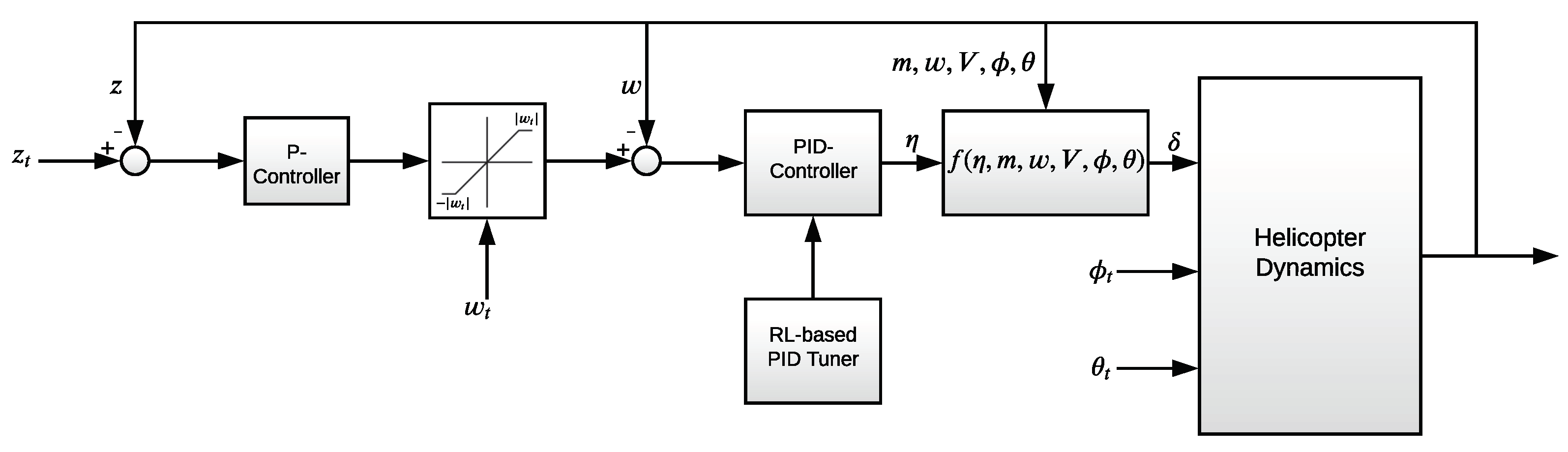
In this study, the control of the longitudinal motion of the helicopter is separated from the lateral motion to ease the trajectory generation process. In the control structure, the vertical and horizontal motion are managed by the thrust level and the rotor roll angle , respectively. Additionally, the speed of the helicopter is adjusted by setting the rotor pitch angle . The proposed control structure is presented in Figure 1.
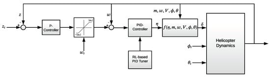
Figure 1.
Control structure.
The rotor roll command and rotor pitch command are utilized to set the rotor roll angle and rotor pitch angle , respectively. The relation between the commanded target values and the real angles is presented using first-order equations as follows:
For the vertical motion, two commanded target values are defined, i.e., the target altitude and the target vertical speed . Both altitude and vertical speed are managed by adjusting the thrust level via the successive loop closure approach. While the inner loop in Figure 1 is used to set the vertical speed, the outer loop is designed to manage the altitude. Because there is a natural integrator in the system when controlling the altitude and the open-loop system is fast enough, a proportional controller (P-controller) is sufficient for the outer loop. For the inner loop, a PID controller is proposed to improve both transition and steady-state performance of the closed-loop system. A new control signal is defined, benefiting from the nonlinear dynamic inversion approach, to create a new input–output linear system that makes the linear control techniques usable without any chattering. The function that is derived via nonlinear dynamic inversion is presented as follows:
When the defined function is written into the fifth equation of the system model (i.e., (1) or (3)), it can easily be seen that the new equation will be , which makes the new system input–output linear and easily controlled using the linear control techniques.
In the proposed control structure, the horizontal and vertical motions are uncoupled. When there are changes to the rotor roll angle or rotor pitch angle, the P-PID controller compensates for the impact of the changes on the vertical motion by modifying the thrust level . This makes the closed-loop system appropriate for feasible trajectory generation with random sampling.
3.2. Reinforcement Learning (RL)-Based Robust PID Tuning
When the model parameters are not known precisely and obtained based on an estimation, the control performance can be affected by deviations in the model parameters. A robust PID design can be proposed to mitigate this impact. As illustrated in Figure 1, an RL-based PID tuner is developed to obtain robust PID parameters.
Reinforcement learning (RL) is an approach based on a trial and error process. By interacting with its environment, the RL agent receives rewards and uses these rewards to calculate the overall return for the defined task. When the environment is fully observable, the focused problem can be described as a Markov decision process (MDP).
A Markov decision process (MDP) is a tuple , where:
- S is a set of states;
- A is a set of actions;
- T is a state transition probability function, ;
- r is a reward function, ;
- is a discount factor, which represents the difference in importance between future rewards and present rewards, .
The core problem of MDPs is to find a policy for the decision-maker by maximizing the long-term future reward. A policy is a mapping from states to actions that defines the behavior of an agent:
and long-term reward is presented as:
However, the calculation of contains the rewards in the future, which must be calculated with a strategy that is different from the direct calculation. The expected long-term reward can be used in this process. For this purpose, two different functions are defined. The state-value function of an MDP is the expected return starting from state s, and the following policy :
The action-value function is the expected return starting from state s, taking action a, and the following policy :
Bellman [15] shows that value functions can be decomposed into two parts, namely, immediate rewards and the discounted value of the successor:
Using this property, value functions can be calculated with recursive algorithms. Then, optimal value functions can also be calculated to generate optimal policy. For example, an optimal policy can be generated by using the Bellman optimality equation [15,16], also known as value iteration. However, finding an optimal policy using the Bellman optimality equation requires a huge amount of space and time when the number of states and actions is high. These kinds of recursive methods, such as value iteration and policy iteration [17], make calculations for all of the state-action pairs in working space, so the computation is hard in real implementations. To overcome this computational inefficiency, an alternative strategy called reinforcement learning (RL) comes from the machine learning domain.
Reinforcement learning consists of an active decision-making agent that interacts with its environment to accomplish a defined task by maximizing the overall return. The future states of the environment are also affected by the agent’s actions. This process is modeled as an MDP when there is a fully observable environment. There are various RL methods that can be utilized to provide a solution for an MDP [17]. RL methods define how the agent changes its policy as a result of its experience. The learning process is based on a sampling-based simulation.
In this study, we benefit from the Proximal Policy Optimization (PPO) algorithm [18] as the RL method. It is based on an actor–critic framework in which two different neural networks are used: actor and critic. While the critic estimates the value function, the actor modifies the policy according to the direction suggested by the critic.
The main idea behind the PPO is to improve the training stability of the policy by limiting the policy change at each training epoch. This is achieved by measuring how much the policy changed with respect to the previous policy using a ratio calculation between the current and previous policy and then clipping this ratio in the range to prevent the current policy from going too far from the former one.
In the PPO, the objective function that the algorithm tries to maximize in each iteration is defined as follows:
where refers to the set of policy parameters. S is the entropy bonus that is used to ensure sufficient exploration. This term encourages the algorithm to try different actions. It can be tuned by setting the constant to achieve the balance between exploration and exploitation. and are constants. is the squared-error value loss, . The term regulates how large the gradient steps can be through gradient clipping. It restricts the range that the current policy can vary from the old one, which is defined as follows:
where is a hyperparameter. The estimated advantage refers to the difference between the discounted sum of rewards and the state-value function. Additionally, symbolizes the probability ratio between the new and the old policy. This ratio measures the difference between the two policies, and it is defined as follows:
where is the old policy.
The PPO algorithm [18] is given below (Algorithm 1). In each iteration, the parallel actors collect the data to compute the average estimates. Additionally, the objective L (17) is maximized via the obtained information by modifying the set of policy parameters based on the stochastic gradient descent. In this way, the policy network is trained iteratively.
| Algorithm 1: PPO Algorithm |
|
The PID tuner is considered to be the RL agent by defining a policy neural network (NN) with a single neuron. The states or the inputs of the policy NN are defined as the error, the derivative of the error, and the error’s integral. Because there is only one layer with a single neuron, each signal is multiplied by a coefficient, i.e., and , when the bias unit is discarded. Additionally, the reward is defined as the negative of the absolute error. The concept of domain randomization [19] is utilized to consider the variability and create a robust structure during the training. In domain randomization, the different aspects of the domain are randomized in the samples used during the training to ensure simulation variability and address the reality gap. In this study, we benefit from domain randomization by giving random deviations to the model parameters during the training. After completing the training process, the coefficients in the policy NN are assigned as the corresponding PID parameters. In this way, a robust set of parameters for the PID controller is obtained by considering random model parameter uncertainties during the training process.
3.3. Simulation Results
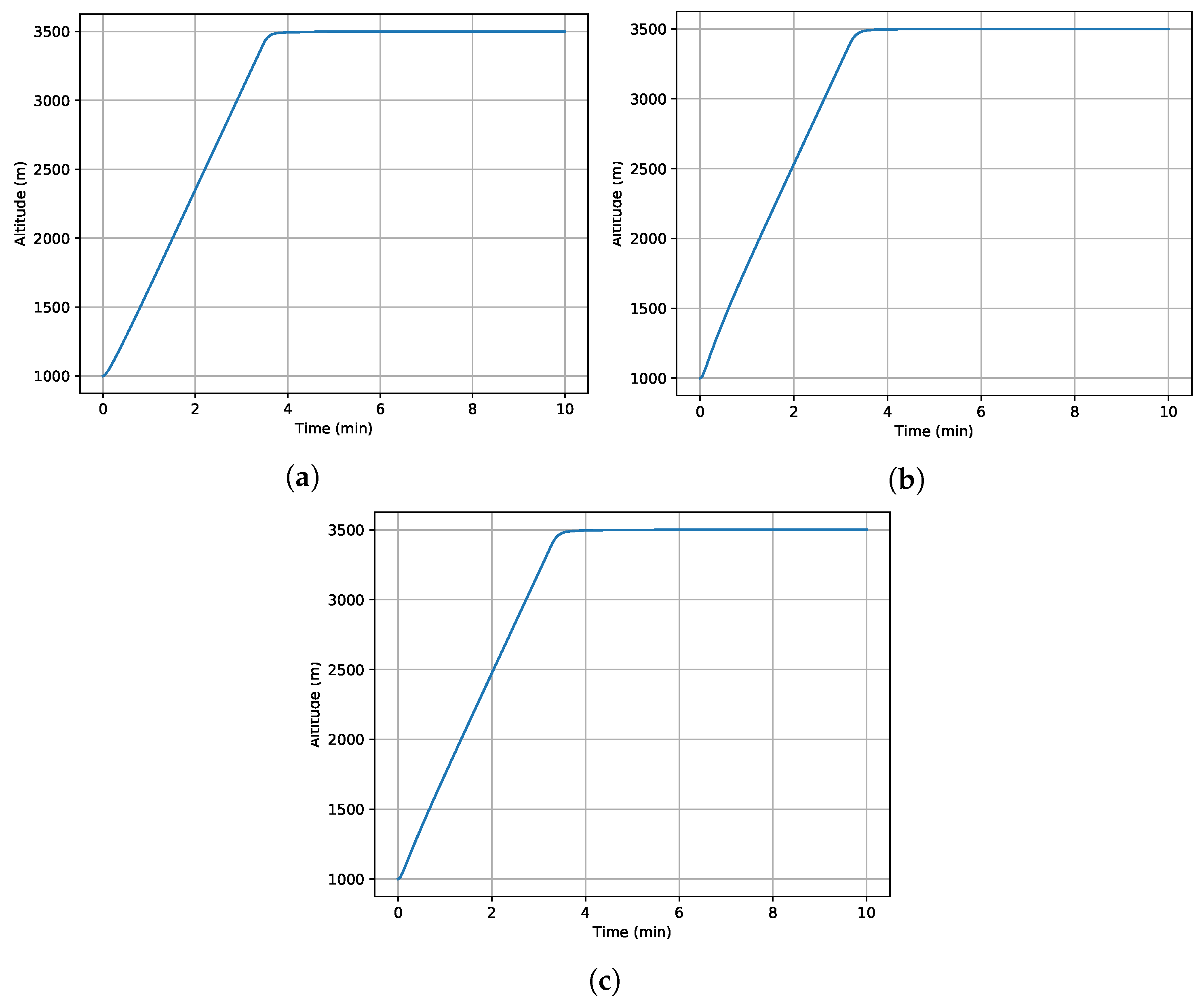
Many different scenarios have been assessed to analyze the performance of the proposed control architecture against the model parameter uncertainty. Parameters and in Equation (10) are considered during the robustness assessment. As illustrative examples, the results of three case studies are presented in Figure 2 and Figure 3. In these case studies, the initial speed of the helicopter is set to zero, and the maximum rotor pitch angle is applied. While the helicopter is in hover at the beginning of the simulation, it accelerates and switches from hover to forward flight. Then, it continues accelerating to a speed of in forward flight. In this way, it experiences both hover and forward flight during simulations. In the first case study, all parameters are considered with deviation, and deviation is applied to all parameters in the second case. The third case study gives different deviations to the with respect to others to show that it is the main parameter that drives the system’s robustness.

Figure 2.
Time history of altitude with different parameter uncertainties, = 3500 m. (a) deviation for all parameters. (b) deviation for all parameters. (c) deviation for and deviation for the rest.
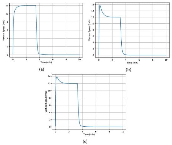
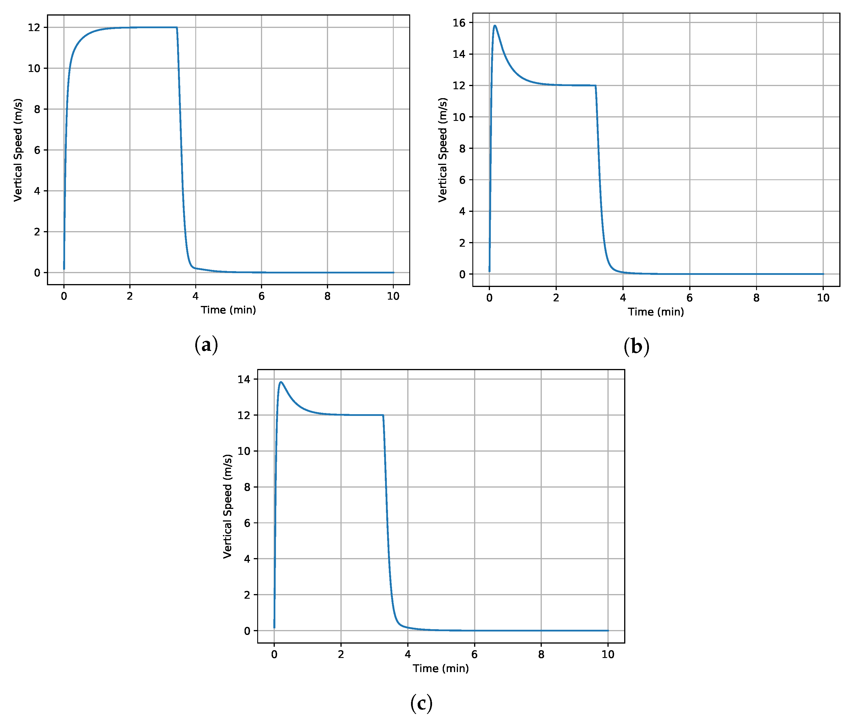
Figure 3.
Time history of vertical speed with different parameter uncertainties, = 12 m/s. (a) deviation for all parameters. (b) deviation for all parameters. (c) deviation for and deviation for the rest.
Overall, the altitude can be controlled without any overshoot or steady-state error. The deviations in the model parameters have almost no impact on the performance of the altitude control, as illustrated in Figure 2. However, there could be an overshoot on the vertical speed, which is controlled without a steady-state error. Especially, the uncertainty in can lead to an overshoot with almost no impact on the settling time.
4. AI-Aided Terrain Avoidance
The proposed model with a robust control structure can be used in any sampling-based algorithm to solve any problem related to trajectory-based operations and intelligent avionics. As a specific case study, we focus on the terrain avoidance problem to illustrate how the model can be used in these types of problems and provide an AI-assisted practical solution for terrain avoidance.
4.1. Model Training
The study benefits from artificial intelligence, specifically, the previously presented proximal policy optimization (PPO) algorithm, to train a policy neural network to be able to solve the terrain avoidance problem.
The RL algorithm is described in the previous section, and the closed-loop helicopter system is utilized to simulate the motion of the agent in the simulation environment. Next, the reward function, state, and action spaces must be defined to be able to train the RL agent for terrain avoidance.
The action space has to consist of the control inputs of the helicopter, which are defined as the target altitude , target vertical speed , target roll angle , and target rotor pitch angle . These variables are normalized between and 1. Then, the action space for the RL agent is defined as follows:
where and are the maximum altitude and vertical speed, respectively.
The state space has to contain all information about the task and the helicopter’s current state. It is specified as follows:
where is the current position of the helicopter, and is the target location. z is the altitude, and is the heading angle of the helicopter. L is the predefined distance to define the region of interest, and it is used to normalize the distances. and are the relative distance and relative course with respect to the destination. is a vector with 25 elements and presents the relative altitude of the helicopter with respect to the terrain elevations in 3 km perimeters.
In the focused problem, the helicopter aims to reach a target region by ensuring terrain avoidance. To increase the convergence speed in the training process, a reward function is defined based on the distance to the destination region as follows:
In this way, the helicopter approaches the target area by trying to decrease the high negative rewards.
When the helicopter reaches the destination area, the simulation is terminated, and a positive reward is given as follows:
Moreover, when the helicopter leaves the predefined area, a negative reward is given to prevent redundant searches in distant areas as follows:
The same negative reward is also given when the helicopter collides with the terrain. An episode is terminated whenever the agent leaves the predefined region, reaches the target, or collides with the terrain during training.
4.2. Simulation Results
The RL agent is trained using the terrain elevation map in Figure 4a. Initial and target positions are defined to describe a trajectory planning problem. The initial position and target location are also illustrated in Figure 4a with a black asterisk and blue asterisk, respectively. For the initial conditions and target position , the helicopter must fly over the mountain illustrated as a yellow area in Figure 4a to be able to reach the destination point. The horizontal projection of the generated trajectory by the trained agent is presented in Figure 4a,b. The output shows that the helicopter reaches the target region by using the shortest path. Additionally, the helicopter’s altitude and the corresponding terrain elevation are presented in Figure 4c. The results show that the helicopter is able to avoid the terrain and reach the target location successfully.
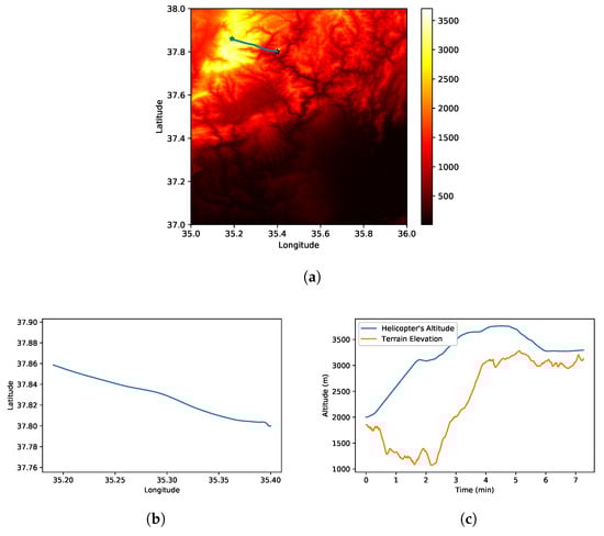
Figure 4.
Simulation results for helicopter terrain avoidance. (a) Terrain elevation map. (b) Horizontal projection of the trajectory. (c) Helicopter’s altitude and terrain height.
5. Conclusions
In this study, we presented a generic helicopter model that includes hover and forward flight regimes for helicopter applications that will be solved via sampling-based methods. A robust controller architecture was presented to enhance the generalizability of the proposed model and overcome the limitations of the open-loop model. The robustness was ensured by benefiting from reinforcement learning for tuning the controller parameters. The simulation results showed that the proposed system generates satisfactory outputs. Hence, it can be utilized in realistic applications. As an illustrative application, AI-assisted terrain avoidance was provided. It was shown that the proposed AI-assisted approach can be used efficiently with the developed model and that it generates practical results for a realistic problem.
The possible trajectories of the helicopter can be assessed by using the proposed model when it is required to evaluate the possible options in a safety-critical situation. It is mandatory for the sampling-based algorithms to check the dynamic limitations using a computationally efficient model. The proposed model ensures this requirement for trajectory-based helicopter operations. Although the main application is presented as terrain avoidance, the proposed system can be used in any trajectory-related helicopter operations or intelligent avionics. It can be utilized in any application that requires a fast, simple, and accurate helicopter dynamics model. It is also applicable to different types of helicopters.
Funding
This research received no external funding.
Data Availability Statement
The terrain elevation data used in this study can be downloaded from the EarthExplorer (http://earthexplorer.usgs.gov/).
Conflicts of Interest
The author declares no conflict of interest.
Abbreviations
The following abbreviations are used in this manuscript:
| AI | Artificial Intelligence |
| RL | Reinforcement Learning |
| PPO | Proximal Policy Optimization |
| NN | Neural Network |
| FF | Forward Flight |
| HV | Hover |
| P-controller | Proportional Controller |
| PID-controller | Proportional Integral Derivative Controller |
References
- Padfield, G.D. Helicopter Flight Dynamics: The Theory and Application of Flying Qualities and Simulation Modelling; John Wiley & Sons: Hoboken, NJ, USA, 2008. [Google Scholar]
- Johnson, W. Helicopter Theory; Courier Corporation: Chelmsford, MA, USA, 2012. [Google Scholar]
- Gavrilets, V.; Mettler, B.; Feron, E. Dynamic Model for a Miniature Aerobatic Helicopter; MIT-LIDS report # LIDS-P-2579; Massachusetts Institute of Technology: Cambridge, MA, USA, 2003. [Google Scholar]
- Tijani, I.B.; Akmeliawati, R.; Legowo, A.; Budiyono, A.; Abdul Muthalif, A. H∞ robust controller for autonomous helicopter hovering control. Aircr. Eng. Aerosp. Technol. 2011, 83, 363–374. [Google Scholar] [CrossRef]
- Ullah, I.; Pei, H.L. Fixed time disturbance observer based sliding mode control for a miniature unmanned helicopter hover operations in presence of external disturbances. IEEE Access 2020, 8, 73173–73181. [Google Scholar] [CrossRef]
- Halbe, O.; Spieß, C.; Hajek, M. Rotorcraft Guidance Laws and Flight Control Design for Automatic Tracking of Constrained Trajectories. In Proceedings of the 2018 AIAA Guidance, Navigation, and Control Conference, Kissimmee, FL, USA, 8–12 January 2018; p. 1343. [Google Scholar]
- Yomchinda, T.; Horn, J.; Langelaan, J. Flight path planning for descent-phase helicopter autorotation. In Proceedings of the AIAA Guidance, Navigation, and Control Conference, Portland, OR, USA, 8–11 August 2011; p. 6601. [Google Scholar]
- Senzig, D.A.; Boeker, E.R. Rotorcraft Performance Model (RPM) for Use in AEDT; Technical report; John A. Volpe National Transportation Systems Center (US): Cambridge, MA, USA, 2015. [Google Scholar]
- Mouillet, V.; Phu, D. BADA Family H-A Simple Helicopter Performance Model for ATM Applications. In Proceedings of the 2018 IEEE/AIAA 37th Digital Avionics Systems Conference (DASC), London, UK, 23–27 September 2018; pp. 1–8. [Google Scholar]
- Baspinar, B. A Generic Model of Nonlinear Helicopter Dynamics for Intelligent Avionics Systems and Trajectory Based Applications. In Proceedings of the AIAA SCITECH 2022 Forum, San Diego, CA, USA, 3–7 January 2022; p. 2100. [Google Scholar]
- Lee, A.Y.; Bryson, A.E., Jr.; Hindson, W.S. Optimal landing of a helicopter in autorotation. J. Guid. Control. Dyn. 1988, 11, 7–12. [Google Scholar] [CrossRef]
- Dooley, L.; Yeary, R. Flight Test Evaluation of the High Inertia Rotor System; Technical report; Bell Helicopter Textron Inc: Fort Worth, TX, USA, 1979. [Google Scholar]
- Dalamagkidis, K. Autonomous Vertical Autorotation for Unmanned Helicopters; University of South Florida: Tampa, FL, USA, 2009. [Google Scholar]
- Sastry, S. Nonlinear Systems: Analysis, Stability, and Control; Springer Science & Business Media: New York, NY, USA, 2013; Volume 10. [Google Scholar]
- Bellman, R. Dynamic Programming; Courier Corporation: North Chelmsford, MA, USA, 2013. [Google Scholar]
- Bellman, R. A Markovian decision process. J. Math. Mech. 1957, 6, 679–684. [Google Scholar] [CrossRef]
- Sutton, R.S.; Barto, A.G. Reinforcement Learning: An Introduction; MIT Press: Cambridge, MA, USA, 1998; Volume 1. [Google Scholar]
- Schulman, J.; Wolski, F.; Dhariwal, P.; Radford, A.; Klimov, O. Proximal policy optimization algorithms. arXiv 2017, arXiv:1707.06347. [Google Scholar]
- Tobin, J.; Fong, R.; Ray, A.; Schneider, J.; Zaremba, W.; Abbeel, P. Domain randomization for transferring deep neural networks from simulation to the real world. In Proceedings of the 2017 IEEE/RSJ international conference on intelligent robots and systems (IROS), Vancouver, BC, Canada, 24–28 September 2017; pp. 23–30. [Google Scholar]

Disclaimer/Publisher’s Note: The statements, opinions and data contained in all publications are solely those of the individual author(s) and contributor(s) and not of MDPI and/or the editor(s). MDPI and/or the editor(s) disclaim responsibility for any injury to people or property resulting from any ideas, methods, instructions or products referred to in the content. |
© 2023 by the author. Licensee MDPI, Basel, Switzerland. This article is an open access article distributed under the terms and conditions of the Creative Commons Attribution (CC BY) license (https://creativecommons.org/licenses/by/4.0/).