Numerical Simulation of Transonic Compressors with Different Turbulence Models

Abstract

One of the most commonly used techniques in aerospace engineering is the RANS (Reynolds average Navier–Stokes) approach for calculating the transonic compressor flow field, where the accuracy of the computation is significantly affected by the turbulence model used. In this work, we use SA, SST, k-ɛ, and the PAFV turbulence model developed based on the side-biased mean fluctuations velocity and the mean strain rate tensor to numerically simulate the transonic compressor NASA Rotor 67 to evaluate the accuracy of turbulence modeling in numerical calculations of transonic compressors. The simulation results demonstrate that the four turbulence models are generally superior in the numerical computation of NASA Rotor 67, which essentially satisfies the requirements of the accuracy of engineering calculations; by comparing and analyzing the ability of the four turbulence models to predict the aerodynamic performance of transonic compressors and to capture the details of the flow inside the rotor. The errors of the Rotor 67 clogging flow rate calculated by the SA, SST, k-ɛ, and PAFV turbulence models with the experimental data are 0.9%, 0.8%, 0.7%, and 0.6%, respectively. The errors of the calculated peak efficiencies are 2.2%, 1.6%, 0.9%, and 4.9%. The SA and SST turbulence models were developed for the computational characteristics of the aerospace industry. Their computational stability is better and their outputs for Rotor 67 are comparable. The k-ɛ turbulence model calculates the pressure ratio and efficiency that are closest to the experimental data, but the computation of its details of the flow field near the wall surface is not ideal because the k-ɛ turbulence model cannot accurately capture the flow characteristics of the region of high shear stresses. The PAFV turbulence model has a better prediction of complex phenomena such as rotor internal shock wave location, shock–boundary layer interaction, etc., due to the use of a turbulent velocity scale in vector form, but the calculated rotor efficiency is small.

1. Introduction

The high−load transonic compressor is one of the core components of an aero-engine. Complex phenomena include shock–boundary layer interaction, non−constant blade tip leakage vortices, and inter-stage disturbances in multi-stage pressured airflow in transonic compressors. Due to the complexity of the flow field inside the compressor, experimental investigations can capture part of the compressor’s critical data, but they are also often very expensive and unable to attain the flow details in the flow field’s rapidly changing conditions. Therefore, computational fluid dynamics (CFD) is increasingly being applied to the design and performance prediction of impellers [1]. Considering the timeliness and economy of engineering calculations, the RANS method is still the mainstream method for solving the N–S equation in practical engineering [2]. The accuracy of the RANS equations’ solution is significantly influenced by the turbulence model; hence, it is crucial to design effective turbulence models in a focused approach.

Spotts et al. [3] investigated the effects of six turbulence models on the numerical calculations of the NASA Rotor 67 transonic compressor based on the RANS method. The findings demonstrate that the turbulence models significantly influence predictions of the transonic compressor’s aerodynamic performance and the shock–boundary layer interaction; the SST and SA turbulence models produce better numerical simulation results close to the stall point, whereas the k-ɛ turbulence model exhibits poor computational stability close to the stall point. The TUDa−GLR−OpenStage data set, which is based on the transonic compressor Darmstadt test facility at the Technical University of Darmstadt, was made available by Klausmann et al. [4]. It offers a new generalized arithmetic example for numerical computing and algorithm verification of compressors. He et al. [5,6] performed numerical simulations of the transonic axial flow compressor NASA Rotor 67 using the SA−QCR model, SA−RC model, SA−H model, and SA−PG model to compare the effects of the latest modified Spalart–Allmaras turbulence model on the performance prediction of the compressor. It is demonstrated that the SA−H and SA−PG turbulence models still have some shortcomings despite having higher computational accuracy than the SA−QCR and SA−RC turbulence models. Using an optical aerodynamic test stand, Brandstetter et al. [7] investigated the operating circumstances, such as transonic and subsonic velocities, of high−speed compressors and identified several potential causes for rotational stall and blade chatter. Foret et al. [8] used a newly created variable stator in series with the BLISK rotor to study how different rotors affected the compressor’s aerodynamic properties. It has been demonstrated that fewer stator blades can produce a larger stator blade load while also increasing the rotor’s operating factor. Zhang et al. [9] investigated the impact of a magazine treatment system with various circumferential coverage ratios on the aerodynamic performance of a centrifugal compressor by performing a non−constant numerical simulation of a Krain impeller based on the RANS method. The results show that the stability of the flow inside the compressor can be improved by circumferential treatment of the magazine, and the stall margin improvement is becoming better with the increase of the circumferential coverage ratio. Using five turbulence models—the offset k-ω turbulence model for non-equilibrium effects proposed by Olsen and Coakley, the standard k-ω turbulence model, the RAG k-ω model, the SST−CC model, and the EARSM model—Liu et al. [10] numerically computed the SRV2-O transonic centrifugal impeller. The results show that the offset k-ω turbulence model for non-equilibrium effects gives better numerical simulation results for transonic centrifugal impellers. To study the performance of a centrifugal compressor machine with high curvature flow, among other things, Ali et al. [11] used three turbulence models. They found that the SST turbulence model was better at predicting the stall region while the SST−CC turbulence model was better at predicting the compressor machine performance curve. Using the Spalart–Allmaras turbulence model, Moreno et al. [12] carried out numerical simulations on an axial compressor and assessed the variables influencing the numerical results. It was shown that the destruction term in the SA model can have an impact on the stall margin loss. Simoes [13], Liu [14], Zhang [15], and Chen [16] et al. have conducted some further insightful investigations on the impact of turbulence models on the numerical simulation of transonic compressors.

The ability of the turbulence model to simulate the effects of all unsteadiness in the mean flow field, including the transfer and dissipation of turbulent energy and the evolution of turbulent vortices, has a significant impact on the accuracy of RANS-based transonic compressor performance prediction. The development of more effective and accurate turbulence models for complicated flow fields, such as transonic compressors, is a more active research subject because the majority of the existing turbulence models have certain flaws. In this paper, Numeca software was used for meshing, the Python program was used for numerical calculations, and Tecplot and Oringin were used for data post−processing. In this study, the newly developed PAFV turbulence model is programmed using a Python program, using PAFV, SA, SST, and k-ɛ turbulence models to numerically calculate the NASA Rotor 67 transonic compressor rotor under different operating conditions based on a grid−independent study. On the characteristic curves of the compressor, the radial temperature and pressure distribution of the rotor inlet and outlet, the distribution of the flow field, and the flow details, the effects of various turbulence models are compared and examined.

2. Computational Models

NASA Rotor 67, the first fan rotor in a two-stage fan designed and experimentally tested by NASA in the late 1980s, is a typical small spreading ratio transonic axial compressor rotor. The algorithm is frequently used to assess the computational accuracy of CFD software/codes due to the availability of considerably more specific geometrical parameters and experimental data, as well as the fact that the flow inside it is a representation of transonic fans. As shown in Figure 1 and Figure 2, Rotor 67 has 22 large−twisted blades with a cold model tip clearance of 1.016 mm, a design speed of 16,043 r/min, a design total pressure ratio of 1.63, and a design point air flow rate of 33.25 kg/s. The specific geometric and design point parameters are shown in

Table 1. NASA Rotor 67 geometry and design point parameters.

Parameter	Value	Parameter	Value
Inlet diameter	0.514 m	Rotational speed	16,043 RPM
Outlet diameter	0.485 m	Design pressure ratio	1.63
Imported wheel ratio	0.375	Blade tip tangent velocity	429 m/s
Export wheel ratio	0.478	Design of blade tip Ma	1.38
Spread–sine ratio	1.56	Total inlet temperature	15 °C [288 K]
Surface fineness	0.8 μm	Total inlet pressure	101,325 Pa
Radius of blade root guide circle	1.78 mm	Design flow	33.25 kg/s
Blade tip clearance	1 mm	Blockage flow	34.96 kg/s
Number of blades	22

[17,18,19].

3. Control Equations and Numerical Methods

3.1. Control Equations and Turbulence Models

The Favre-averaged Navier–Stokes (N–S) equations and the differential forms of the continuity, momentum, and energy equations in the Cartesian coordinate system serve as the governing equations for the calculations in this work:

$$\frac{\partial \rho }{\partial t}+\frac{\partial \rho u_i}{\partial x_i}=0,$$

(1)

$$\frac{\partial \rho u_j}{\partial t}+\frac{\partial }{\partial x_i}\left(\rho u_j{u}_i+p{\delta }_{ij}-{\tau }_{ij}\right)=S{m}_j,$$

(2)

$$\frac{\partial \rho E}{\partial t}+\frac{\partial }{\partial x_i}\left[\left(\rho E+p\right)u_i+q_i-u_i{\tau }_{ij}\right]=Se,$$

(3)

In the equation:

$${\tau }_{ij}=\left({\mu }_L+{\mu }_T\right){\epsilon }_{ij},$$

$${\epsilon }_{ij}=2S_{ij}-\frac{2}{3}\left(\nabla \cdot \mathit{u}\right){\delta }_{ij},$$

$$S_{ij}=\frac{1}{2}\left(\frac{\partial u_i}{\partial x_j}+\frac{\partial u_j}{\partial x_i}\right),$$

$$E=e+\frac{\mathit{u}·\mathit{u}}{2},$$

$$e=\frac{1}{k-1}RT=\frac{1}{k-1}\frac{p}{\rho },$$

$$q_i=-\lambda \frac{\partial T}{\partial x_i}=-\left(\frac{{\mu }_{\mathrm{L}}}{\mathrm{P}{\mathrm{r}}_{\mathrm{L}}}+\frac{{\mu }_{\mathrm{T}}}{\mathrm{P}{\mathrm{r}}_{\mathrm{T}}}\right)\frac{k}{k-1}\frac{\partial }{\partial x_i}\left(\frac{p}{\rho }\right),$$

Among them are: $\mathit{u}$, $p$, $\rho$, $E$, $e$, $\tau$, $\epsilon$, $S$, ${\mu }_{\mathrm{L}}$, ${\mu }_{\mathrm{T}}$, ${\mathrm{Pr}}_{\mathrm{L}}$, ${\mathrm{Pr}}_{\mathrm{T}}$, $k$. They are velocity, pressure, density, total energy, thermodynamic energy, stress, strain rate, deformation rate, laminar viscosity coefficient, turbulent viscosity coefficient, laminar Prandtl number, turbulent Prandtl number, and the specific heat ratio. $S{m}_j$ and $Se$ in Equations (2) and (3) represent the rotation terms of the momentum equation and the energy equation when calculating the compressor, respectively. The x−axis is the axis of rotation. Their specific expressions are as follows.

$$\left(\begin{array}{c}S{m}_x\\ S{m}_y\\ S{m}_z\end{array}\right)=\left(\begin{array}{c}0\\ \rho {\omega }^{2}y+2\rho \omega w\\ \rho {\omega }^{2}z-2\rho \omega v\end{array}\right),$$

$$Se=\rho {\omega }^2\left(vy+wz\right),$$

where $\omega$, x, y, and z are angular velocity and Cartesian coordinates, respectively.

In the RANS approach, the turbulent viscous coefficients are computed using the turbulence model equations and used to determine the turbulent viscous stresses. The turbulence model equations used in this paper are further described below. This paper develops a partial average fluctuation velocity (PAFV) turbulence model based on group averaging of turbulent fluctuation velocity to solve the set of Navier–Stokes equations after Reynolds averaging. The instantaneous velocity of turbulence can be expressed as $\mathit{u}=\overline{\mathit{u}}+{\mathit{u}}^{\prime }$, where $\overline{\mathit{u}}$ denotes the average velocity of the tether and ${\mathit{u}}^{\prime }$ denotes the corresponding fluctuations velocity. For compressible flows, where density is often coupled with other physical quantities, it is more convenient to use mass-weighted averaging (Favre averaging), and the velocity can be written as $\mathit{u}=\tilde{\mathit{u}}+{\mathit{u}}^{″}$, where $\tilde{\mathit{u}}$ denotes Favre average speed and ${\mathit{u}}^{″}$ denotes the corresponding fluctuations velocity. It is difficult to employ the physically real and significant first-order fluctuations velocities in the turbulence modeling process because the average value derived by coefficient averaging or Favre averaging of all fluctuation’s velocities at a place in space is zero. For this reason, ${\mathit{u}}^{″}$ is grouped into positive and negative groups based on the mean value $\tilde{\mathit{u}}$ and weighted in such a way that the average information of the non−zero first-order fluctuations velocity can be obtained and called the side-biased mean fluctuations velocity $\widehat{\mathit{u}}$. The side−biased mean fluctuations velocity in turn has a weighted symmetry concerning $\tilde{\mathit{u}}$ [20]. The turbulent velocity scale can be described by the side−biased mean fluctuations velocity, which also possesses vector features. The side−biased mean fluctuations velocity model is better at describing anisotropic fluctuations and transport characteristics of turbulence than the conventional turbulence model because it contains detailed information about the turbulence field.

The new model equations can be obtained by group−weighted averaging of the instantaneous fluctuations velocity equations and modeling the unknown correlation terms. The specific equations are of the form:

$$\frac{\partial \rho {\widehat{u}}_j}{\partial t}+\frac{\partial \rho \left({\widehat{u}}_j{u}_i+{\widehat{u}}_i{u}_j\right)}{\partial x_i}=\frac{\partial \left({\widehat{\tau }}_{ij}-{\tau }_{ij}\right)}{\partial x_i},$$

(4)

In the equation:

$${\widehat{\tau }}_{ij}=\left({\mu }_{\mathrm{L}}+{\mu }_{\mathrm{T}}\right){\widehat{\epsilon }}_{ij},$$

$${\widehat{\epsilon }}_{ij}=2{\widehat{S}}_{ij}-\frac{2}{3}\left(\nabla \cdot \widehat{u}\right){\delta }_{ij},$$

$${\widehat{S}}_{ij}=\frac{1}{2}\left(\frac{\partial {\widehat{u}}_i}{\partial x_j}+\frac{\partial {\widehat{u}}_j}{\partial x_i}\right),$$

where: $\widehat{\mathit{u}}$ is the mean lateral deflection fluctuations velocity; $\widehat{\tau }$, $\widehat{\epsilon }$ are the stress and strain rates constructed by the mean lateral deflection fluctuations velocity, respectively. Equation (2) reveals that the turbulent viscous force term and the molecular viscous diffusion term are responsible for the loss of mean flow volume. In Equation (4), these two terms turn into the sources of turbulent fluctuations velocity generation, converting the momentum of mean flow loss into that of turbulent fluctuations flow. In the three–dimensional flow, the PAFV turbulence model is a three–equation model, by solving the average fluctuations velocity of the side deviation in three directions, and then constructing the turbulent viscosity coefficient, and then obtaining the turbulent stress term, in this paper, constructing the turbulent viscosity coefficient of the form of:

$${\mu }_T=\beta \frac{\rho {\widehat{u}}_i{\widehat{u}}_i}{2S},$$

(5)

$$S=\sqrt{2S_{ij}{S}_{ij}},$$

(6)

In Equation (5), the coefficient $\beta$ is taken from 0.1 to 0.6.

To avoid redundancy, the relevant equations and detailed descriptions of the Spalart–Allmaras turbulence model, the SST k-ω turbulence model, and the k-ɛ turbulence model are described in detail in references [21,22,23]. On the k-ɛ model, the standard k-ɛ model [23] was used in the far field and the Wolfshtein model [24] was used in the near-wall region. The two models are blended according to Ref. [25].

3.2. Numerical Scheme

The Steger–Warming vector flux splitting method, which has the advantages of strong surge capture capability, high reliability, and high computational efficiency, is chosen for the computational transonic pressurizer problem in this paper, taking into account the characteristics of rotation, curvature, and excitation that appear in the computation. The set of turbulence equations is transformed in the general curvilinear coordinate system. The multi-step Runge–Kutta method is used to demonstrate the time advance solution approach for the constant flow problem of the compressor, and the local time step method is employed to increase computation efficiency while taking into account the non-uniformity of the calculation grid, and CFL number is taken as 0.05. The spatial discretization is in the third-order upwind scheme and the temporal discretization is in the third-order Runge–Kutta method. The computations were programmed in Python based on the discrete methods and control equations mentioned above.

Numerical calculations were performed for different operating conditions by giving the outlet radial equilibrium static pressure. The convergence of the steady-state simulations can be measured by observing the stability of the pressure ratio, efficiency, and mass flow rate of the Rotor 67 for a given backpressure, as well as the level of normalized residuals present at the end of the simulation. Typically, the calculated normalized residuals are reduced by at least 4-order.

3.3. Computational Grids and Boundary Conditions

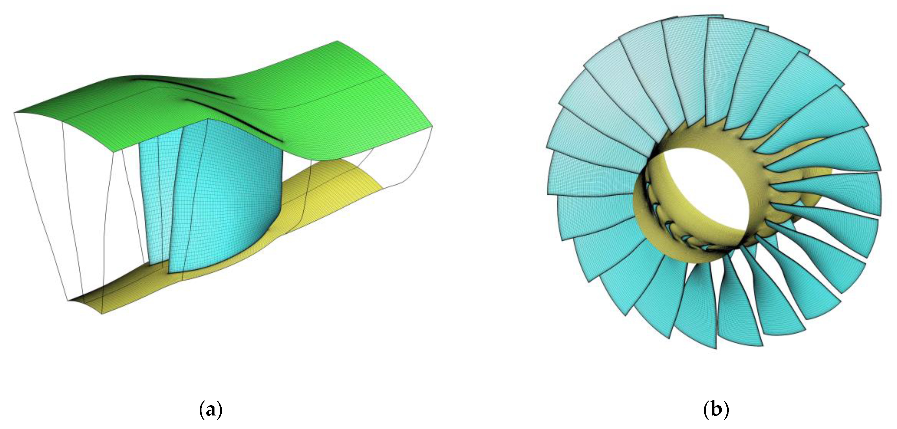
In this paper, a single-channel simulation is used in the calculation, the Rotor 67 rotor model is meshed using Numeca software, and a high–quality structured mesh is divided based on the multiple meshing technique. Figure 3 depicts the computational domain and wall meshes (grid lines are separated for easy inspection). The height of the first layer of the wall mesh satisfies 1.5 × 10⁻⁶, and the Y⁺ of the first layer of the blade wall, hub, cassette, and blade tip positions is between 1 and 10.

The inlet boundary, exit boundary, solid wall boundary, and periodic boundary make up the boundaries of the Rotor 67 rotor single–pass computational domain. The inlet boundary is set to subsonic axial inlet, given a total temperature of 288.15 K, a total pressure of 101,325 Pa, and an inverse static pressure, and the lateral deflection pulsation velocity in the turbulence model is set to 0. The lateral deflection pulsation velocity of the turbulence model is also extrapolated, and the outflow boundary is set to a specified mean static pressure, density, and velocity. The relative velocity is provided as 0, the static pressure and density are extrapolated, the hub and blades in the solid wall boundary are set to adiabatic no–slip in the rotating coordinate system, and the magazine is set to adiabatic no–slip in the stationary coordinate system. The single-channel computational domain grid is periodically matched, and linear interpolation is used on the rotating periodic boundary to obtain the parameters on the boundary. See Appendix A for more details on boundary conditions.

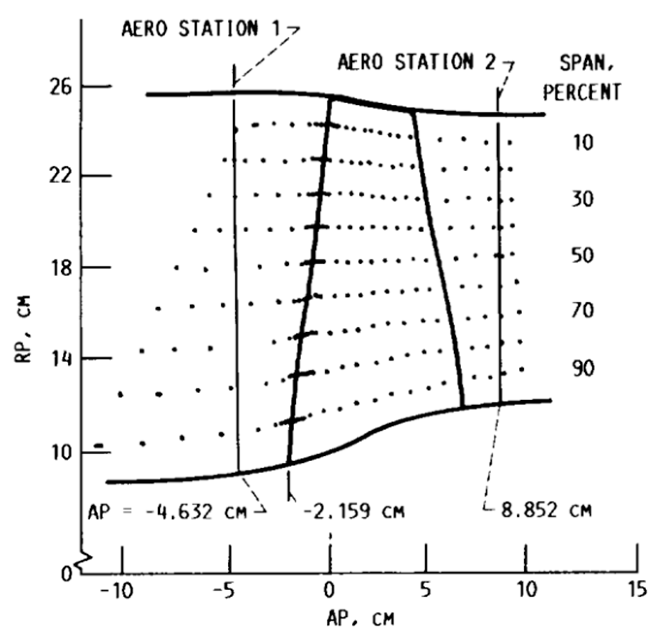
The inlet and outlet measurement sites for the Strazisar et al. [26]. Tests are depicted in Figure 4, and this is where the data for the characteristic line and radial exit parameters in this investigation are derived from.

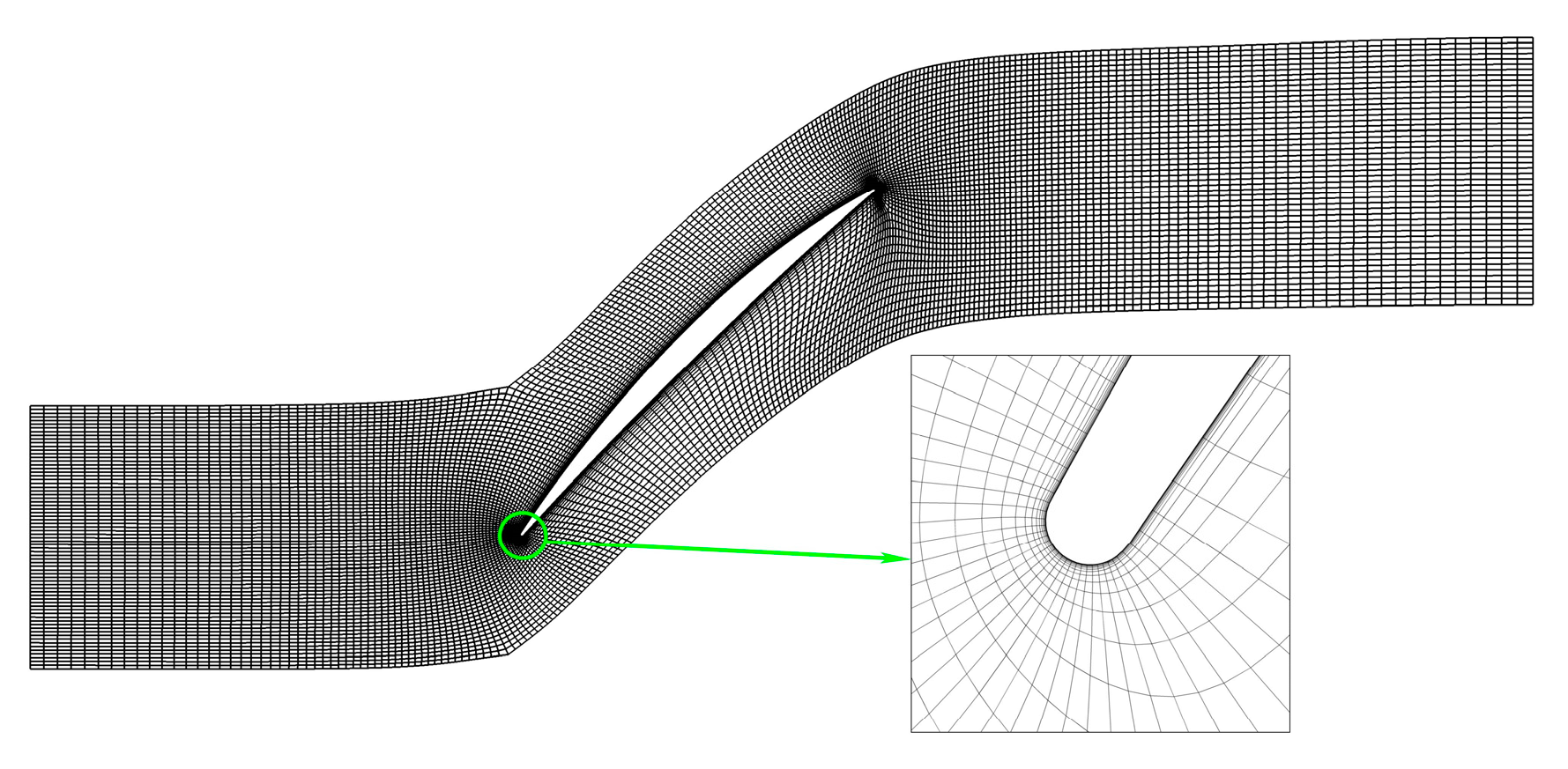
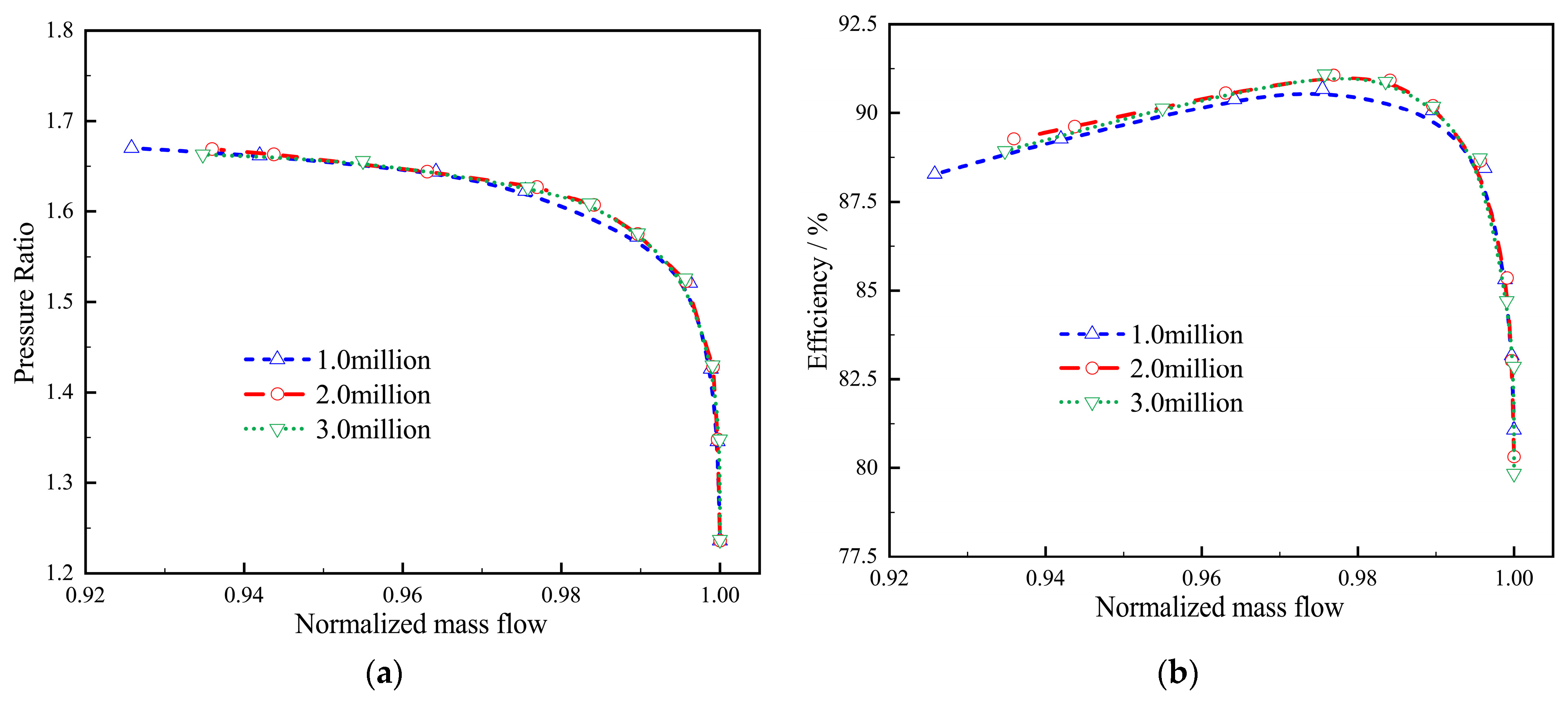
In this paper, numerical calculations were performed on a 32-core computer, using Microsoft MPI for parallel calculations. For a grid of 2 million, the computational time used for a given back pressure is about 3–4 h. To reduce the influence of the mesh on the calculation results, the mesh independence of the Rotor 67 model was verified for three sets of coarse, medium, and fine meshes, using the S−A model. The total grid numbers of the three sets of different sparsity grids are 1 million (69 × 73 × 217, circumferential × axial × radial grid numbers), 2 million (73 × 133 × 217), and 3 million (81 × 153 × 257), where the B2B surfaces and meridional of the 2 million grid are shown in Figure 5 and Figure 6. Figure 7 displays the Rotor 67 pressure ratio and efficiency characteristic lines. From Figure 7, it can be seen that the calculated results of the 1 million grid differ slightly from the other two sets of denser grids, while the results of the 2 million and 3 million grids are the same. Integrating computational accuracy and computational efficiency, this paper subsequently uses a grid of 2 million grid points.

4. Analysis of Calculation Results

4.1. Compressor Performance Curve

Table 2. Comparison of pressurizer performance data calculated from four turbulence models with experimental values.

	Blockage Flow (kg/s)	Near Stall Point Pressure Ratio	Maximum Efficiency	Design Point Efficiency
S-A	34.65	1.669	91.06%	90.21%
SST	34.66	1.683	91.70%	90.40%
k-ɛ	34.72	1.676	92.30%	91.00%
PAFV	34.76	1.661	88.60%	87.30%
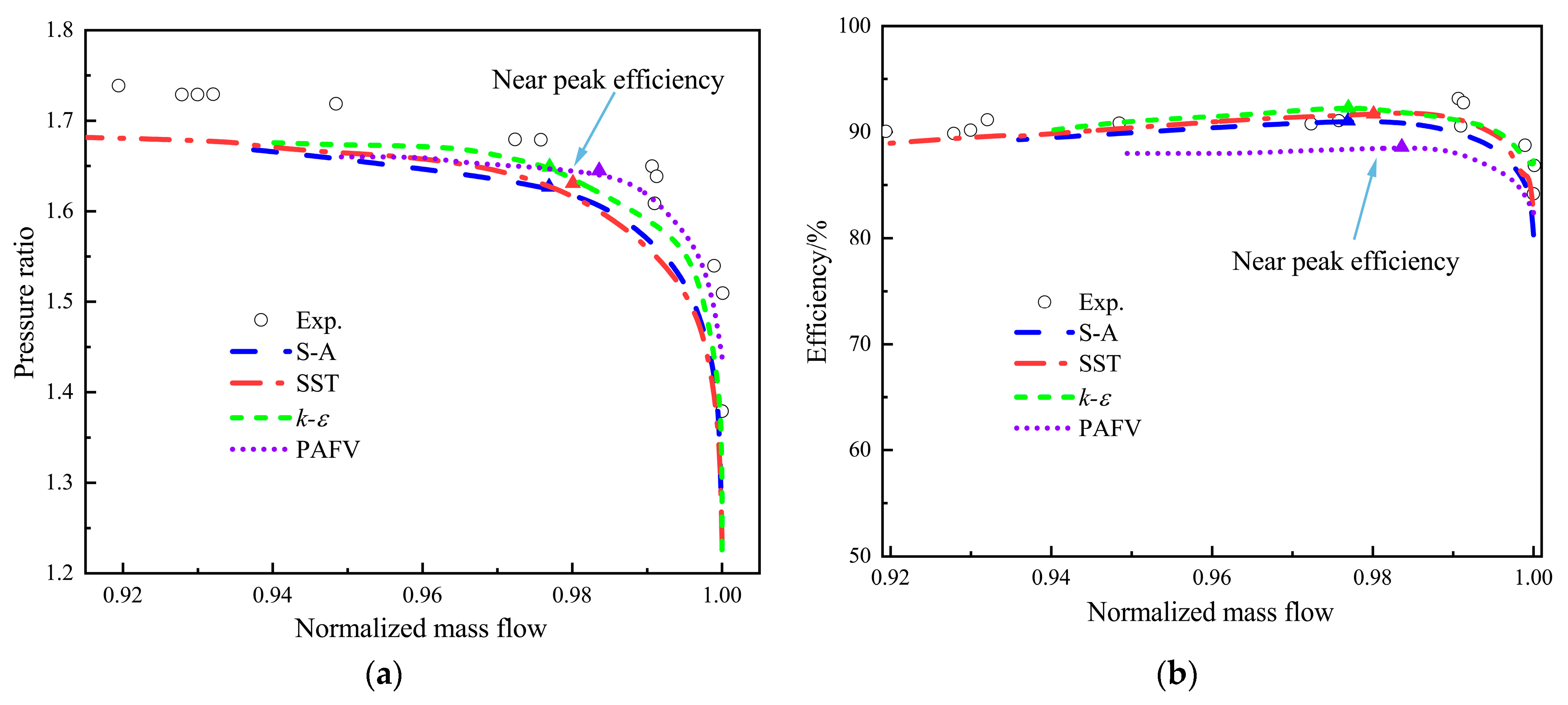
Exp.	34.96	1.728	93.18%	90.58%

lists the key performance information for the compressor derived from the four turbulence models, and Figure 8 displays the NASA Rotor 67 flow–total pressure ratio variation curves and flow–efficiency variation curves for the design settings. The efficiency curves typically match the experimental results, and the calculated total pressure ratio data are slightly lower than the experimental values, as can be seen in Figure 8, where the calculated results of the four turbulence models are generally more consistent with the experimental data. The k-ɛ turbulence model is closest to the experimental results, and the flow rate, as well as the pressure ratio range calculated by the SST turbulence model, is larger than the other three turbulence models. The S−A is close to the calculated results of the SST turbulence model but slightly smaller than the SST turbulence model, and the pressure ratio results calculated by the PAFV turbulence model are close to the k-ɛ turbulence model, but the efficiency curve is smaller than the other three turbulence models, which may be caused by the excessive friction loss on the blade surface and requires further improvement of the relevant parameters of the turbulence model subsequently. According to the performance curves, the peak efficiency of Rotor 67 predicted by the four turbulent models is approximately 98% of the blockage flow conditions, which is consistent with results predicted in the literature [3] and experimentally measured by Strazisar et al. [26] at 99% of the blockage flow conditions. The S−A turbulence model deviates the most from the experimental values with an error of about 0.9%, and the PAFV turbulence model is closest to the experimental values with an error of about 0.6%, as can be seen in Table 2. The numerically calculated Rotor 67 blockage flows are all slightly smaller than the experimental values. The experimentally measured near–stall point pressure ratio is slightly higher than the numerical calculation, and the SST is closest to the experimental value with an error of about 2.6%, followed by the k-ɛ and SA turbulence models, and the PAFV turbulence model has the largest difference from the experimental value. The SST turbulence model is the closest to the experimental results with an error of about 0.6%, and the PAFV turbulence model is the most different from the experimental values with an error of about 4%. For the efficiency of the Rotor 67 compressor design point, the calculated results of all three turbulence models are slightly lower than the experimental values, except the k-ɛ turbulence model, which is slightly higher.

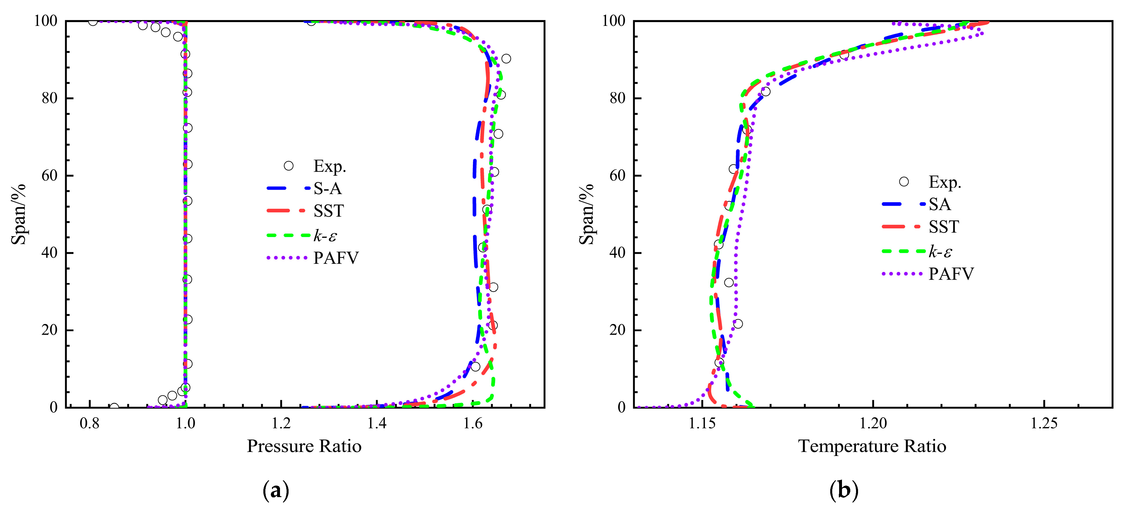
Figure 9 shows the radial distribution of the total pressure ratio and total temperature ratio calculated by the four turbulence models at near–peak efficiency conditions. Figure 9a shows the radial distribution of the inlet and outlet total pressure ratio under near peak efficiency conditions. Inlet and outlet pressure ratios derived by the four turbulence models at peak operating conditions do not significantly differ, as seen in Figure 9a, and the general trend coincides well with the actual results, with a few minor deviations in the specifics. The PAFV turbulence model’s pressure ratio curves are closest to the experimental results at the outlet, and the results of the other three turbulence models are also comparable. However, the k-ɛ turbulence model performs slightly worse at the root of the blade near the hub, which may be because it does not accurately represent the flow characteristics of the high–shear stress region close to the wall. Figure 9b shows the radial distribution of the total outlet temperature for near–peak efficiency conditions, and it can be seen from the figure that the total temperature ratios calculated by all four turbulence models are in good agreement with the experimental results.

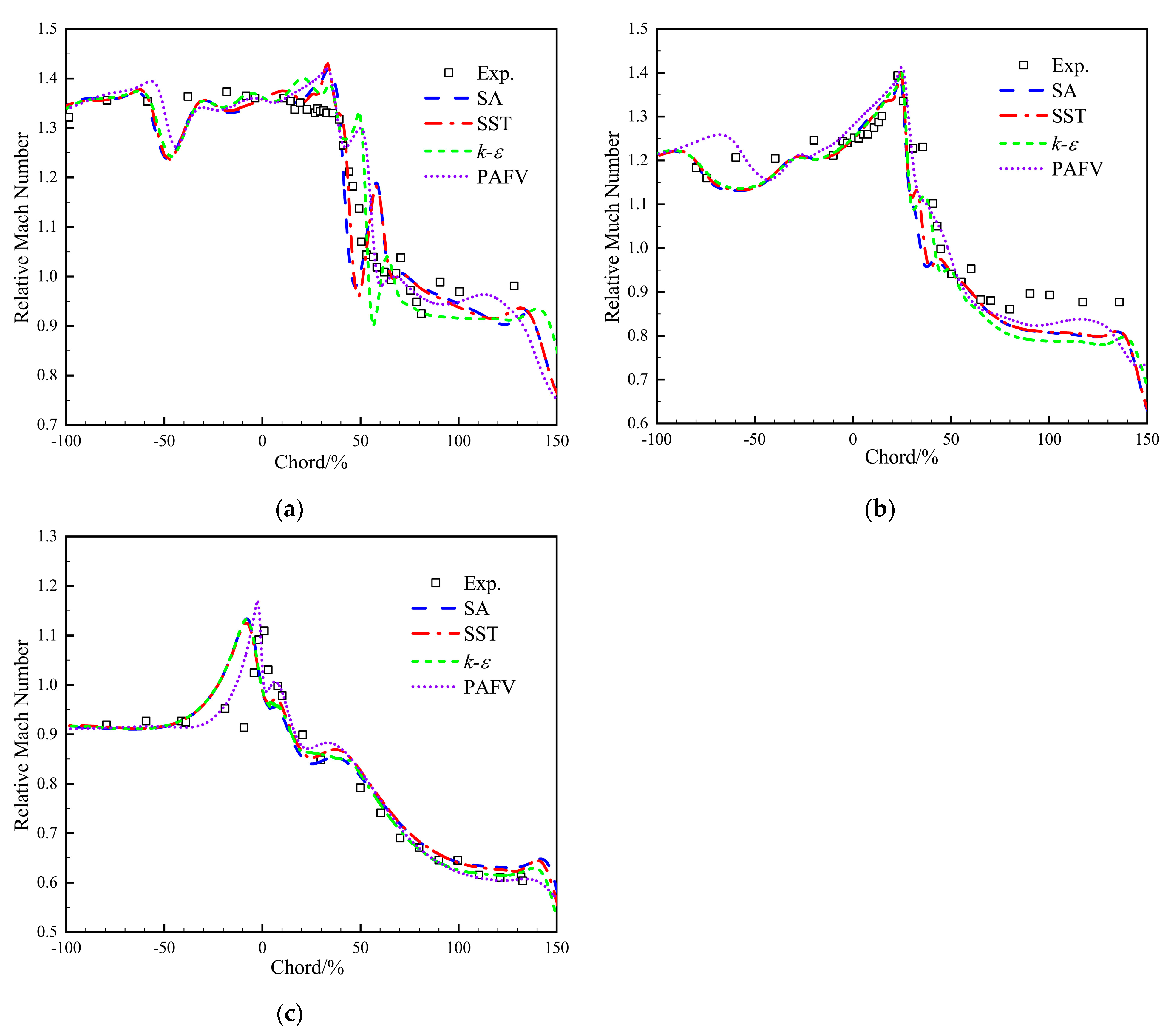
Figure 10 shows the Mach number distribution for different lobe heights at near peak efficiency points with 50% pitch and is also compared with experimental data. The relative Ma number distribution at 90% blade height, 70% blade height, and 30% blade height are shown in Figure 10a–c, respectively. The chord length of the blade of the corresponding section in the image makes the horizontal coordinates dimensionless, and 0% chord length and 100% chord length, respectively, indicate the leading edge and trailing edge portions of the blade. Overall, the Mach number distributions calculated by the four turbulence models are in good agreement with the experimental results, and all of them predict the fluctuation of Mach number along the flow direction more accurately, which may be because the cross–section of 50% grid pitch is farther away from the blade and less influenced by the flow field on the blade surface. The Mach number calculations for the wake region at 70% and 90% of the blade height for all four turbulence models contain some errors, indicating that they are unable to predict the flow field conditions in the wake region at higher blade heights, which is consistent with the calculation results reported in the literature [15]. There is a strong channel shock wave in the blade channel, and the higher the blade, the greater the velocity, the stronger the shock wave, and this situation is more clearly shown in Figure 10a,b. At 50% grid pitch and 30% blade height, the channel shock wave is in the leading edge area of the blade near 0% of the chord length. At 70% blade height, the channel shock wave develops to about 25% of the leading edge of the blade. At 90% blade height, the channel shock wave is further enhanced. In the area of about 40% of the middle of the blade, this channel shock wave results in a relatively large loss in the overall efficiency of the computer. At the 50% grid pitch, a weak shock wave gradually appears before the airflow enters the blade channel as the blade height increases and the velocity in the flow field increases, and this weak shock wave gradually increases with the increase of the blade height. The SA, SST, and k-ɛ turbulence models have similar calculations for this weak shock wave location, and the PAFV turbulence model is slightly worse than the other three turbulence models.

In Figure 10c, at 30% span from the hub, the calculated results of the PAFV turbulence model match the experimental data more closely than the other three turbulence models. Particularly at the channel shock wave, the PAFV turbulence model predicts the position of the channel shock wave more accurately, and the positions of the channel shock wave calculated by the SA, SST, and k-ɛ turbulence models are slightly earlier than the experimental value.

4.2. Computational Flow Field Analysis

Figure 11 shows the calculated results of the Mach number distribution inside the 70% blade height channel compared with the experimental results. The four turbulence models’ calculated results are consistent with the flow characteristics inside the transonic rotor, according to Mach number cloud plots at various blade heights. The numerical results are also in good agreement with the experimental results, and the flow field characteristics are essentially consistent with the development trend. In the flow field channel at 70% blade height, normal shock waves and oblique shock waves occur, and the pressurization of the transonic flow is accomplished by these two shock waves. The obvious interference phenomenon of the shock–boundary layer interaction also arises on the suction surface of the blade in the flow field channel at 70% of the blade height.

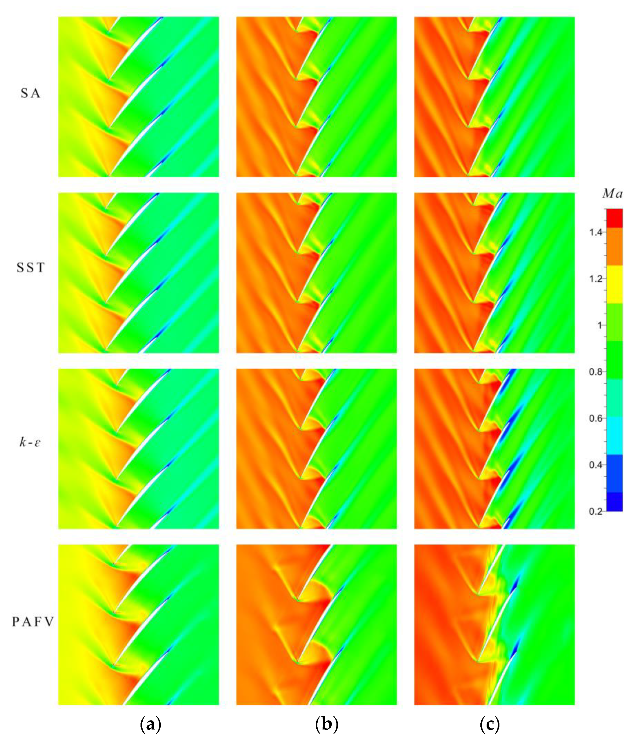
The Mach number cloud plots at 60% blade radius, 90% radius, and 95% radius as computed by several turbulence models are shown in Figure 12 at Rotor 67’s peak efficiency. The graphic shows that all four turbulence models compute the Mach number flow field more accurately and that as the radius grows, the shock wave phenomenon is significantly enhanced in all four turbulence models’ calculations. In addition to the shock wave at the blade’s leading edge, the shock wave in the blade channel is also more noticeable around 90% of the blade radius position, and there is a particular phenomenon known as shock–boundary layer interaction. The associated layers on both sides converge to form the trailing trail of the blade as the airflow moves from the blade’s concave side and the blade’s convex side to the trailing edge, respectively. Among the four turbulence models, the SA and SST turbulence models are closest to one another in terms of calculation outcomes, such as the placement of the shock waves in the flow field. Due to its inadequacy close to the wall, the k-ɛ turbulence model predicts the Rotor 67 blade wake area with a more noticeable low–speed section. The PAFV turbulence model predicts the details of the flow field in a richer way, especially in the portion of the gap near the top of the blade, which has a very complex flow field. The results of the PAFV turbulence model are more in line with the actual flow field, demonstrating that the PAFV turbulence model is capable of a better computation for the complex flow field of the transonic compressors.

When the Rotor 67 rotor is operating at a point close to its peak efficiency, as illustrated in Figure 13, the flow field at the top gap of the blade predicted using the PAFV turbulence model can be seen, and the tip leakage vortex is indicated by the red arrow in the figure. The second tip leakage vortex is shown by the black arrow, which is consistent with the two Mach number fluctuations fluctuating in the middle of the 30–70% blade at the 50% pitch 90% blade height in Figure 10a. The reason for its generation may be caused by the shock–boundary layer interaction. The shock–boundary layer interaction basically occurs at the same location where the second blade tip leakage vortex is generated. This interaction results in a local separation because of the shock–boundary layer interaction, and this separation causes the blade tip leakage flow to roll up the second blade tip leakage vortex.

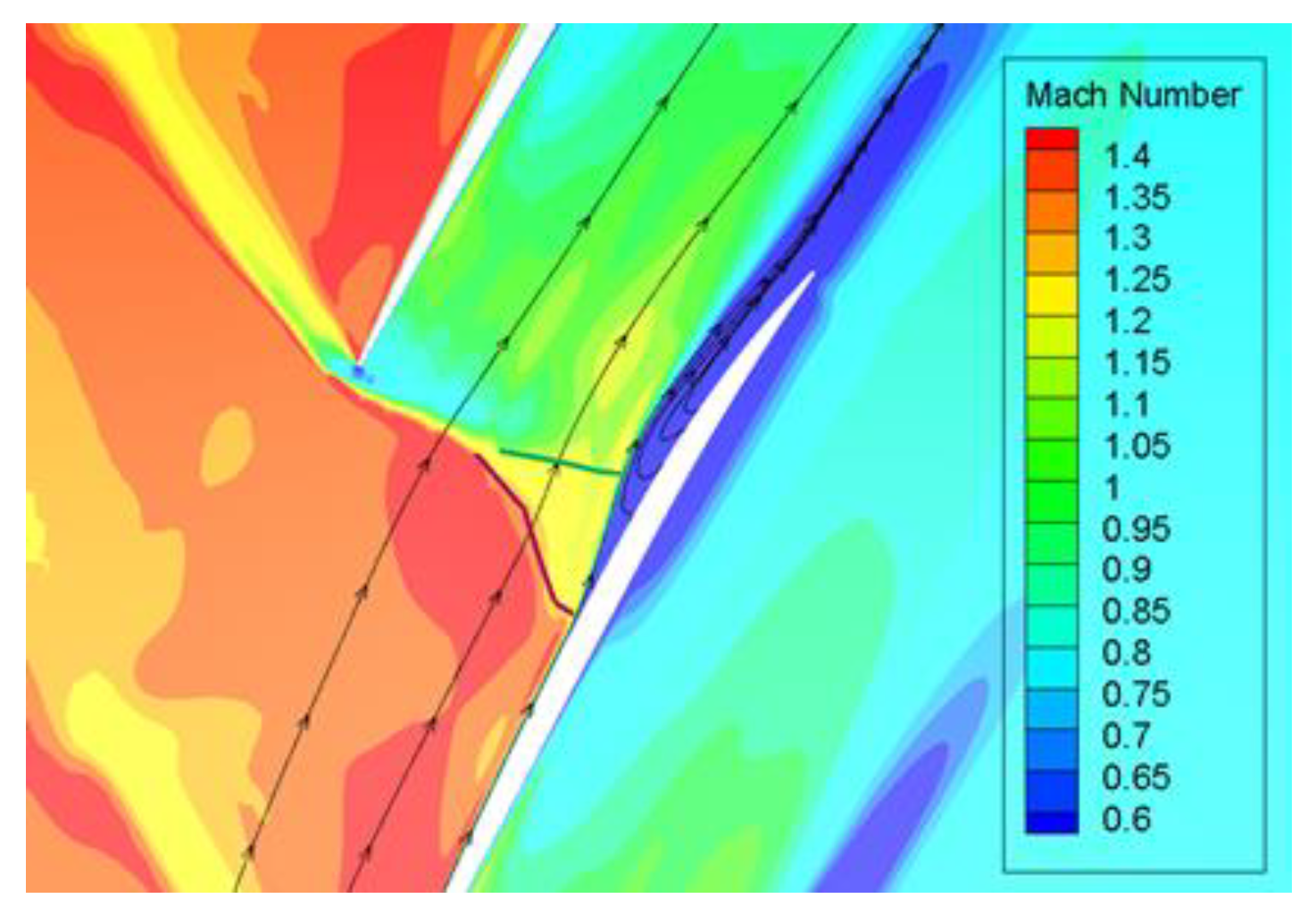
The shock–boundary layer interaction phenomenon on the blade suction surface at the peak efficiency point calculated using the PAFV turbulence model is seen in Figure 14. According to the calculation results, obvious transonic flow develops in the compressor under higher back pressure circumstances, and the shock–boundary layer interaction phenomenon is clearly visible on the suction surface of the blades. The inverse pressure gradient generated by the shock wave caused the boundary layer to thicken on the suction surface of the blade, and there is a certain separation so that the shock wave near the suction surface is firstly shifted upstream to form the first shock wave, and then the second shock wave is formed at the location of the maximum separation. The whole surge has a “λ” shape, which is a typical phenomenon in the shock–boundary layer interaction.

5. Conclusions

In this study, four turbulence models—SA, SST, k-ɛ, and the newly developed PAFV—have been used to computationally investigate the aerodynamic performance and flow field characteristics of NASA Rotor 67, a transonic compressor rotor. The following conclusions can be drawn by comparing the characteristic curves, radial distributions of inlet/outlet total pressure ratios, total temperature ratios, Mach-number distributions at various blade heights with a 50% pitch, and the tip flow structure of Rotor 67.

(1) The four turbulence models can generally predict the performance and flow field of the transonic compressor more precisely when the experimental data and calculation results are thoroughly compared. The errors of the Rotor 67 clogging flow rate calculated by the SA, SST, k-ɛ, and PAFV turbulence models with the experimental data are 0.9%, 0.8%, 0.7%, and 0.6%, respectively. The errors of the calculated peak efficiencies are 2.2%, 1.6%, 0.9%, and 4.9%, respectively, and the results of the numerical calculations basically satisfy the need for accuracy in engineering calculations at the design point of a transonic compressor.

(2) In calculating the performance curves of Rotor 67, the SST turbulence model can capture the turbulence structure more accurately in the near–wall region due to the hybrid form of k-ω and k-ɛ turbulence models and also provides better turbulence prediction in the free–flowing region. Therefore, the performance curve calculated by the SST turbulence model is generally slightly better than the other three turbulence models. The results of the PAFV turbulence model are similar to the SST when calculating the pressure ratio curves, but slightly worse than those of the other three turbulence models in the efficiency curves. The radial distributions of the inlet/outlet total pressure ratios and total temperature ratios calculated by the SA, SST, and PAFV turbulence models are more in line with the experimental results. The k-ɛ turbulence model gives slightly poorer predictions of the total pressure ratio near the hub wall due to its poor ability to capture flow details in the high shear stress region near the wall.

(3) Due to the use of a velocity scale in vector form, the PAFV turbulence model more accurately captures the anisotropy of the turbulence. As a result, the PAFV turbulence model predicts the channel shock waves more accurately at low blade heights and provides better calculation of the flow details related to the interaction between the leakage vortex and the shock waves in the tip section. Both the SA and SST turbulence models are more accurate in their calculations and similarly predict the position of the shock wave. On the other hand, the k-ɛ turbulence model predicts a larger wake thickness near the tip of the blade compared to the experimental results.

References

1. Sandberg, R.D.; Michelassi, V. Fluid dynamics of axial turbomachinery: Blade-and stage-level simulations and models. Ann. Rev. Fluid Mech. 2022, 54, 255–285. [Google Scholar] [CrossRef]
2. Mani, M.; Dorgan, A.J. A perspective on the state of aerospace computational fluid dynamics technology. Ann. Rev. Fluid Mech. 2023, 55, 431–457. [Google Scholar] [CrossRef]
3. Spotts, N.; Gao, X. Comparative Study of Turbulence Models for RANS Simulations of Rotor 67. In Proceedings of the 54th AIAA Aerospace Sciences Meeting, San Diego, CA, USA, 4–8 January 2016. [Google Scholar]
4. Klausmann, F.; Franke, D.; Foret, J.; Schiffer, H.P. Transonic compressor Darmstadt-Open test case Introduction of the TUDa open test case. J. Glob. Power Propuls. Soc. 2022, 6, 318–329. [Google Scholar] [CrossRef]
5. He, X.; Zhao, F.; Vahdati, M. Uncertainty Quantification of Spalart-Allmaras Turbulence Model Coefficients for Simplified Compressor Flow Features. J. Fluids Eng. 2019, 142, 9. [Google Scholar] [CrossRef]
6. He, X.; Zhao, F.; Vahdati, M. Evaluation of Spalart-Allmaras Turbulence Model Forms for a Transonic Axial Compressor. In Proceedings of the GPPS Chania20, Chania, Greece, 7–9 September 2020. [Google Scholar]
7. Brandstetter, C.; Juengst, M.; Schiffer, H.P. Measurements of Radial Vortices, Spill Forward, and Vortex Breakdown in a Transonic Compressor. J. Turbomach. 2018, 17, 12–18. [Google Scholar] [CrossRef]
8. Foret, J.; Franke, D.; Klausmann, F.; Klausmann, F.; Schneider, A.; Schiffer, H.P.; Becker, B.; Muller, H. Experimental Aerodynamic and Aeroelastic Investigation of a Highly-Loaded 1.5-Stage Transonic Compressor with Tandem Stator. Int. J. Tubomach. Propuls. Power 2021, 6, 21. [Google Scholar] [CrossRef]
9. Zhang, H.; Wang, H.; Li, Q.; Jing, F.; Chu, W. Mechanism Underlying the Effect of Self-Circulating Casings with Different Circumferential Coverage Ratios on the Aerodynamic Performance of a Transonic Centrifugal Compressor. Aerospace 2023, 10, 312. [Google Scholar] [CrossRef]
10. Liu, Z.; Wang, P.; Zhao, B.; Yang, C. Assessment of a novel k–ω turbulence model for transonic centrifugal impeller simulations. Trans. Can. Soc. Mech. Eng. 2022, 46, 3. [Google Scholar] [CrossRef]
11. Ali, S.; Elliott, K.J.; Savory, E.; Zhang, C.; Martinuzzi, R.J.; Lin, W. Investigation of the Performance of Turbulence Models with Respect to High Flow Curvature in Centrifugal Compressors. J. Fluids Eng. 2016, 138, 5. [Google Scholar] [CrossRef]
12. Moreno, J.; Dodds, J.; Vahdati, M.; Stapelfeldt, S. Deficiencies in Turbulence Modelling for the Prediction of the Stability Boundary in Highly Loaded Compressors. In Proceedings of the ASME Turbo Expo 2019: Turbomachinery Technical Conference and Exposition, Phoenix, AZ, USA, 17–21 June 2019. [Google Scholar]
13. Simoes, M.R.; Montojos, B.G.; Moura, N.R.; Su, J. Validation of turbulence models for simulation of axial flow compressor. In Proceedings of the 20th International Congress of Mechanical Engineering, Gramado, Brazil, 15–20 November 2009. [Google Scholar]
14. Liu, Y.; Yan, H.; Liu, Y.; Lu, L.; Li, Q. Numerical study of corner separation in a linear compressor cascade using various turbulence models. Chin. J. Aeronaut. 2016, 29, 639–652. [Google Scholar] [CrossRef]
15. Zhang, Q.; Huang, X.; Wang, D. Evaluation of Different Spalart–Allmaras Turbulence Models for Turbomachinery Flow Field Analysis. J. Propuls. Tech. 2022, 43, 4. (In Chinese) [Google Scholar]
16. Chen, X.; Koppe, B.; Lange, M.; Chu, W.; Mailach, R. Comparison of turbulence modeling for a compressor rotor at different tip clearances. AIAA J. 2022, 60, 1186–1198. [Google Scholar] [CrossRef]
17. Urasek, D.C.; Gorrel, W.T.; Cunnan, W.S. Performance of Two-Stage Fan Having Low-Aspect-Ratio, First-Stage Rotor Blading; Technical Paper 1493; NASA: Cleveland, OH, USA, 1979.
18. Cunnan, W.S.; Stevans, W.; Urasek, D.C. Design and Performance of a 427-Meter-per-Second-Tip-Speed Two-Stage Fan Having a 2.40 Pressure Ratio; Technical Paper 1314; NASA: Cleveland, OH, USA, 1978.
19. Suder, K.L.; Hathaway, M.D.; Okiishi, T.H.; Strazisar, A.J.; Adamczyk, J.J. Measurements of the Unsteady Flow Field within the Stator Row of a Transonic Axial-Flow Fan: I—Measurement and Analysis Technique; Technical Memorandum 88945; NASA: Cleveland, OH, USA, 1987.
20. Gao, G.; Yong, Y. On incompressible turbulent flow: Partial average based theory and applications. J. Hydraul. Res. 2005, 43, 399–407. [Google Scholar] [CrossRef]
21. Spalart, P.R.; Allmaras, S.R. A one-equation turbulence model for aerodynamic flows. In Proceedings of the AIAA 30th Aerospace Sciences Meeting and Exhibit, Reno, NV, USA, 6–9 January 1992. [Google Scholar]
22. Menter, F.; Rumsey, C. Assessment of two-equation turbulence models for transonic flows. In Proceedings of the Fluid Dynamics Conference, Colorado Springs, CO, USA, 20–23 June 1994. [Google Scholar]
23. Launder, D.B.; Spalding, D.B. The numerical computation of turbulent flows. Comput. Methods Appl. Mech. Eng. 1974, 3, 2. [Google Scholar] [CrossRef]
24. Wolfshtein, M. The Velocity and Temperature Distribution in one-Dimensional Flow with Turbulence Augmentation and Pressure Gradient. Int. J. Heat Mass Transfer 1969, 12, 301–308. [Google Scholar] [CrossRef]
25. Jongen, T. Simulation and Modeling of Turbulent Incompressible Flows. Ph.D. Thesis, EPF Lausanne, Lausanne, Switzerland, 1992. [Google Scholar]
26. Strazisar, A.J.; Wood, J.R.; Hathaway, M.D.; Suder, K.L. Laser Anemometer Measurements in a Transonic Axial-Flow Fan Rotor; Technical Paper 2879; NASA: Cleveland, OH, USA, 1989. [Google Scholar]
Figure 1. Photograph of NASA Rotor 67.
Aerospace 10 00784 g001
Figure 2. Geometric model of NASA Rotor 67.
Aerospace 10 00784 g002
Figure 3. Computational domain and overall grid of NASA Rotor 67 (a) channel grid; (b) NASA Rotor 67 integral grid.
Aerospace 10 00784 g003
Figure 4. Laser measurement map of NASA Rotor 67 meridian plane [26].
Aerospace 10 00784 g004
Figure 5. B2B surface mesh.
Aerospace 10 00784 g005
Figure 6. Meridian mesh.
Aerospace 10 00784 g006
Figure 7. Performance curves for NASA Rotor 67 were calculated using three different sets of grids. (a) Pressure ratio; (b) efficiency.
Aerospace 10 00784 g007
Figure 8. Performance curves of NASA Rotor 67 calculated by four turbulence models versus experimental values. (a) Pressure ratio (b) efficiency.
Aerospace 10 00784 g008
Figure 9. Radial distribution of total pressure ratio and total temperature ratio for near-peak efficiency conditions. (a) Radial distribution of the total pressure ratio of inlet and outlet; (b) radial distribution of the total outlet temperature.
Aerospace 10 00784 g009
Figure 10. Radial distribution of total pressure ratio and total temperature ratio for near–peak efficiency conditions. (a) 90% span from the hub; (b) 70% span from the hub; (c) 30% span from the hub.
Aerospace 10 00784 g010
Figure 11. Mach number distribution in the 70% blade height channel. (a) SA model; (b) SST model; (c) k-ɛ model; (d) PAFV model; (e) Exp.
Aerospace 10 00784 g011
Figure 12. Mach number clouds at peak efficiency are calculated by different turbulence models. (a) 60% span from the hub; (b) 90% span from the hub; (c) 95% span from the hub.
Aerospace 10 00784 g012
Figure 13. Flow field distributions in the blade top gap are calculated by the PAFV turbulence model.
Aerospace 10 00784 g013
Figure 14. Surge boundary layer interference phenomena in PAFV turbulence model calculations.
Aerospace 10 00784 g014