Article

Multi-Objective Bayesian Optimization Design of Elliptical Double Serpentine Nozzle

School of Power and Energy, Northwestern Polytechnical University, Xi’an 710129, China
*
Author to whom correspondence should be addressed.
Aerospace 2024, 11(1), 48; https://doi.org/10.3390/aerospace11010048
Submission received: 16 November 2023 / Revised: 18 December 2023 / Accepted: 29 December 2023 / Published: 31 December 2023

Abstract

:
The use of traditional optimization methods in engineering design problems, specifically in aerodynamic and infrared stealth optimization for engine nozzles, requires a large number of objective function evaluations, therefore introducing a considerable challenge in terms of time constraints. In this paper, this limitation is addressed by using a sample-efficient multi-objective Bayesian optimization that takes Kriging as a surrogate model and Expected Hypervolume Improvement as the infill criterion. Using this approach, the probabilistic model is continuously established and updated, and the approximate Pareto front is obtained at a relatively small computational budget. The objective of this work is to evaluate the applicability of employing a multi-objective Bayesian optimization framework for the aerodynamic-infrared shape optimization of an elliptical double serpentine nozzle at 6 km flight condition, where the objective functions are evaluated by means of high-fidelity computational fluid dynamics and reversed Monte Carlo ray tracing simulations. We achieve good results in both infrared radiation signature reduction and aerodynamic performance improvement with a reasonable number of evaluations, indicating that the proposed method is effective and efficient for tackling the computationally intensive optimization challenges in the aircraft design.

1. Introduction

With the development of infrared (IR) tracking and detection technology, the infrared stealth characteristics of the new-generation fighter will meet new challenges. As an important component of the engine, the nozzle provides the majority of the thrust, while the high-temperature, high-velocity plume and hot parts inside the nozzle make it the primary infrared radiation within the aircraft [1]. In order to enhance the survivability and overall combat proficiency, extensive research [2,3,4] has been conducted on their infrared radiation signature and aerodynamic characteristics, which have naturally become the focus of research.
Traditionally, aircraft nozzle typically feature a circular inlet and circular exit with a straight transition of flow from inlet to exit. However, the growing demands for stealth capabilities in fighter aircraft and the drive to reduce noise in civil aircraft have shifted researchers’ attention from the conventional axisymmetric nozzle to the asymmetric nozzle [5]. The potential of serpentine nozzles for IR suppression has led to their implementation in a series of stealth bombers and unmanned aerial vehicles (UAVs) [6,7,8]. The asymmetric shape of these nozzles allows for better mixing between the hot exhaust gas and the surrounding atmosphere, which can result in a shorter high-temperature potential core length of the exhaust plume [9,10]. Additionally, the curved design of the nozzle helps hide the major hot sections of the engine, such as the turbine section and central cone, thereby further contributing to the reduction of the IR signature [11]. On average, the IR radiation intensity can be reduced by at least 70 % compared to a circular nozzle [12]. Typically, for the serpentine nozzle, there is often a significant reduction in the IR signature in the axial direction, while relatively higher signature levels are observed on the sides and below the nozzle when the aspect ratio of the nozzle increases [13].
According to the literature mentioned above, it is known that the serpentine nozzle with a non-circular exit can effectively decrease the infrared radiation emitted by the high-temperature walls and exhaust gases. However, the transition from a circular inlet to a non-circular exit, as well as the axial centerline curvature, can induce secondary flows inside the nozzle [5]. These secondary flows can significantly complicate the flow field, potentially leading to detrimental effects on the aerodynamic performance of the nozzle. Rajkumar et al. [14] conducted an experiment to analyze the flow characteristics of a shallow single serpentine curved convergent nozzle under different pressure ratios. The results indicated an initial deceleration of the flow due to the turning of streamlines caused by the nozzle curvature, as well as an acceleration of the core flow due to the geometric transition. Furthermore, the vortices induced by separation from the tailcone and the sidewall vortices have a significant impact on the temperature distribution of the nozzle [15,16]. This effect becomes particularly prominent in the instance of double serpentine nozzles, where regions with high temperature, often termed as hot streaks, tend to develop along the nozzle surface. These high-temperature zones will cause material degradation of the nozzle and adversely affect the IR stealth capabilities of the nozzle [17,18].
Generally, simulations of the aerodynamic and IR characteristics of the nozzle require high-performance computing resources and advanced numerical methods. Simultaneously altering the values of all design factors of interest, while considering both aerodynamic and infrared characteristics, would considerably increase the computational workload. Therefore, most previous research on the elliptical double serpentine nozzle has focused on analyzing the influence of a single design factor or objective, which makes the conclusion limited. However, with the growing need for advanced stealth technology, there is an increasing demand for multi-objective design approaches that can simultaneously improve aerodynamic performance and reduce IR signatures [19,20]. Conventional multi-objective optimization methods, such as Genetic Algorithms (GAs) require a considerably large number of objective function evaluations, rendering them impractical for this optimization problem due to the associated computational intensity [21,22].
This study aims to present a sample-efficient hybrid design optimization framework based on multi-objective Bayesian optimization (BO) to improve the infrared stealth characteristics of the serpentine nozzle while still emphasizing the enhancement of aerodynamic performance, which has significant engineering application potential and exploration value. The lengths of the first and second “S” sections and the aspect ratio of the nozzle exit are selected as the design variables. These are changed simultaneously during the iteration of the optimization. The rest of the paper is organized as follows: the parametric design of an elliptical double serpentine nozzle is first outlined in Section 2. A comprehensive optimization framework based on Bayesian optimization is presented in Section 3. A Bayesian-based multi-objective optimization framework is applied to optimize the shape of the elliptical double serpentine nozzle and the optimized models are compared with the baseline model in Section 4. Finally, the conclusions are summarized in Section 5.

2. Model

2.1. Nozzle Design Methodology

The exhaust system under investigation comprises three primary sections: the exhaust mixer, the serpentine nozzle and the straight section. Based on a two-spool mixed flow turbofan engine at the design point, the exhaust mixer with two ducts is established. The hot gases flow through the core, while the low-temperature fluids flow through the bypass. Notably, the elliptical serpentine nozzle improves the stealth performance of the exhaust system in two ways. Firstly, the internal components of the exhaust system are obscured by the nozzle wall, and therefore, the infrared radiation and radar echo received by the detectors are reduced. Secondly, the elliptical-shaped outlet enhances the mixing of external and internal airflow, reducing the high-temperature exhaust gas temperature and thus lowering its infrared radiation. Figure 1 provides a brief description of the geometric parameters of the elliptical exit double serpentine nozzle.
The double serpentine nozzle with an elliptical exit can be divided into two individual single serpentine nozzles by the key section at the first bend. The axial length of the first serpentine section is denoted as L 1 with a vertical offset indicated by Δ Y 1 . The axial length of the second serpentine nozzle is L 2 with vertical offset Δ Y 2 . Then, the offset of the double serpentine nozzle can be expressed as Δ Y 2 Δ Y 1 . Interfacing with the exit of the second serpentine nozzle is the straight section, which can restrict the gas flow and prevent non-uniform flow at the exit, with the length being L 3 . Detailed geometric parameters of the elliptical double serpentine nozzle are shown in Table 1.
Lee [23] proposed three distribution types which have superior aerodynamic performance in the subsonic diffusers. The so-called Lee curve is essentially a series of uniformly changing polynomial curves regulated by Equation (1), which is characterized by a slope of zero at both ends as shown in Figure 2. Given this characteristic, the distribution of area and curvature along the streamwise direction can also be governed by the Lee curve, as defined in Equations (2) and (3), respectively. The secondary flow inside the nozzle is influenced by the transverse pressure gradient, which is controlled by the centerline shapes. The streamwise pressure gradient that caused the flow separation is controlled by area distributions. The curvature distribution regulates the rate of transition from the circular inlet to the elliptical exit. In Equations (2)–(4), L denotes the axial length of the nozzle and x refers to the location of the center along the axis. A i and A e represent the nozzle inlet area and exit area, respectively. κ e and κ i stand for the curvature of the nozzle exit and inlet, respectively. Δ Y is the offset of the serpentine nozzle and y signifies the offset of the i-th section corresponding to the x coordinate. To reduce the loss instigated by flow separation at the first inflection section, the distribution of the centerline of the first serpentine section and the second serpentine section rapidly changes at the entrance and rapidly changes at the exit, respectively. In addition, a moderate area distribution is applied to acquire the section area and curvature for the serpentine nozzle. The specific coefficients for the Lee curve for the area, curvature, and centerline distribution are presented in Table 2.
y = Δ y A x L 2 + B x L 3 + C x L 4
A n A i A e A i = A x L 2 + B x L 3 + C x L 4
κ n κ i κ e κ i = A x L 2 + B x L 3 + C x L 4
y Δ Y = A x L 2 + B x L 3 + C x L 4

Parametrization of Elliptical Serpentine Nozzle
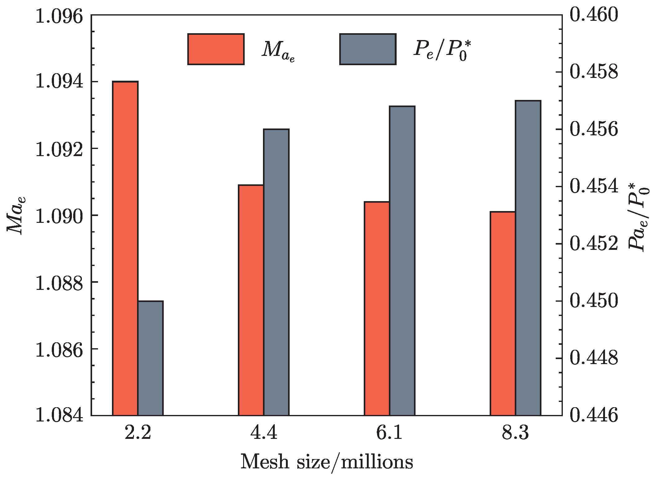
A curvature-based control methodology is employed to generate the sections transitioning from a circular inlet to an elliptical exit. Given a specific nozzle inlet area A i n , nozzle exit area A o u t , and aspect ratio A R of exit ellipse, the inlet and exit can be characterized by N discrete points, respectively.
In order to ensure the smoothness of the solid surface of the elliptical double serpentine nozzle generated in the 3-d construction, the discrete points of the curve imported into the CAD software must be evenly distributed. The uniform distribution of points on the elliptical nozzle exit is achieved by identifying the root of equal arcs length equation for the angle Φ .
To facilitate the transition from circular inlet to the elliptical exit, the curvature κ of inlet and outlet must first be resolved as follows:
κ = ( θ i + 1 θ i ) s a r c , i = [ 0 , 1 , , N 1 ]
where s a r c corresponds to the arc length divided by N points. In this study, N is set to 2000. Subsequently, the curvature of the j - th cross section is represented as:
κ j = κ i n + c j · [ κ o u t κ i n ]
where κ i n and κ o u t denote the curvature of the nozzle inlet and exit, respectively, and c j refers to the curvature distribution controlled by Equation (1). In this study, Equation (4) with coefficients of A = 3, B = −2, C = 0 and A = 4, B = 4 , C = 1 is utilized to govern the curvature distribution of the first section and second section, respectively. It is worth noting that, due to truncation errors, the sum of the radians of each discrete arc length κ j · s may not equal 2 π . This discrepancy implies that the cross section curve is not closed, which can prevent the successful generation of the nozzle wall. This issue can be addressed by applying a minor correction coefficient to each cross section. Once the curvature at each point along the cross section has been established, the coordinate of discrete points along the j-th curve can be iteratively calculated as follows:
θ i = θ i 1 + s j , i 1 · κ j , i 1 x i = x i 1 + s j , i 1 · cos θ i y i = y i 1 + s j , i 1 · sin θ i
Following this, the coordinates of each cross-section are isotropically scaled to the desired area while retaining the same curvature. The area A for each cross-section is defined by Equation (4) with A = 3, B = 2 , C = 0 for the two sections. Finally, based on the nozzle length L, nozzle offset Δ Y , and geometric parameters of the centerline, the final parametric characteristic curve of the serpentine nozzle can be derived by translating and rotating the section curves.

2.2. CFD Method

The outer mold lines around the nozzle are designed to represent an embedded propulsion system, and are aligned with the inflow boundary of the computational domain. A high-precision hexahedral structure grid is used to discretize the computational domain of the elliptical serpentine nozzle. The computational domain includes a rectangular far field bounding box containing free stream flow, with dimensions defined as 10 D × 10 D × 30 D , where D is the diameter of the nozzle entrance, as shown in Figure 3a. Detailed grid configurations on the nozzle inlet and wall are shown in Figure 3b. Spalart–Allmaras (SA), standard k ϵ and shear-stress transport (SST) k ω turbulence model are used to carry out the numerical simulation for the elliptical double serpentine nozzle. Comparative analyses suggest that the SST k ω model can accurately capture the characteristics of the pressure gradient flow and transonic shock wave with high convergence stability. In addition, many previous studies [1,15] have applied a SST k ω turbulence model to the simulation of serpentine nozzles at different boundary conditions and obtained reasonable results. Therefore, the SST k ω turbulence model in the Ansys FLUENT is adopted to simulate the flow characteristics of the elliptical double serpentine nozzle.
The energy, momentum, density, turbulent kinetic energy, and turbulent dissipation rate are discretized using a second-order upwind scheme and the convergence accuracy of each equation is set to 1 × 10 4 . The boundary conditions of the domains in the simulation are defined as follows: no-slip and adiabatic wall boundary conditions are imposed on the solid walls of the nozzle. The discrete ordinates (DO) radiation model is adopted to capture the radiation energies emitted from the solid wall. The external emissivity is set to 0.85 for the nozzle wall, cone and mixer. Pressure-inlet with total pressure and total temperature is applied to the core and bypass of the nozzle. The interior sections are meshed and set as the interior boundary, which is used to monitor the flow during the simulation. All simulations employ a nozzle pressure ratio (NPR) of 3.5 and an entrance temperature ratio of 0.4. The ambient domain is defined as pressure-far-field and the Reynolds number of the nozzle is 4.7 × 10 6 . The simulation is conducted at a flight altitude of 6 km and a cruising Mach number of 0.7, with the nozzle oriented at a zero angle of attack. The detailed values of the boundary conditions are presented in Table 3. A species transport model is selected to determine the spatial distribution of the absorption-emitting gas. The gas from the bypass section is considered to be air, whereas the exhaust gas from the core section is considered to be burned gas, with species properties detailed in Table 4. The arrangement of IR sensors is depicted in Figure 4. Sensors are strategically positioned on the x O y and y O z planes in a circular pattern, spaced at 2-degree intervals around the circumference and located 5 km from the center of the nozzle exit.
In order to satisfy the requirements of the SST k ω turbulence model, a boundary layer has been constructed near the solid wall inside the serpentine nozzle to ensure that y + < 5 . As CFD simulations are time-intensive within the optimization process, solution convergence is accelerated by using the full multi-grid (FMG) initialization, which provides superior initial solutions. During the FMG initialization phase, the inviscid Euler equations are solved using first-order discretization to obtain an approximate solution.
To evaluate the grid size dependence of the numerical results, a grid-sensitive analysis for the serpentine nozzle is carried out. Four grids with different numbers of cells, where the total number of grids escalates from 2 million to 8 million, are simulated to characterize the aerodynamic characteristics of the serpentine nozzle. The ratio of static pressure at the exit to the total pressure at the nozzle inlet, denoted as p e / p 0 , and the Mach number at the exit, represented as M a e , for different grids are extracted and exhibited in Figure 5. It is observed that the values of M a e and p e / p 0 are almost indistinguishable between the medium mesh, dense mesh, and extremely dense mesh. Given that the infrared radiation calculation for the nozzle entails a highly complex ray tracing process, coupled with time-consuming database queries and transmissivity calculations, an increase in the number of cells will significantly escalate the computation time. Therefore, to strike a balance between computational cost and precision, the mesh comprising 4.4 million cells has been selected to accurately capture the flow characteristics and temperature distribution of the elliptical double serpentine nozzle in the optimization process. It is worth noting that the CFD simulation for the grid with 4.4 million cells takes 8 h, whereas the infrared radiation calculation lasted 31 h. Consequently, the entire cycle for one nozzle model requires a total of 39 h. This computational task is executed on a 5.1 GHz Intel Raptor Lake i5-13600K CPU, equipped with 64 GB DDR5 Ram.

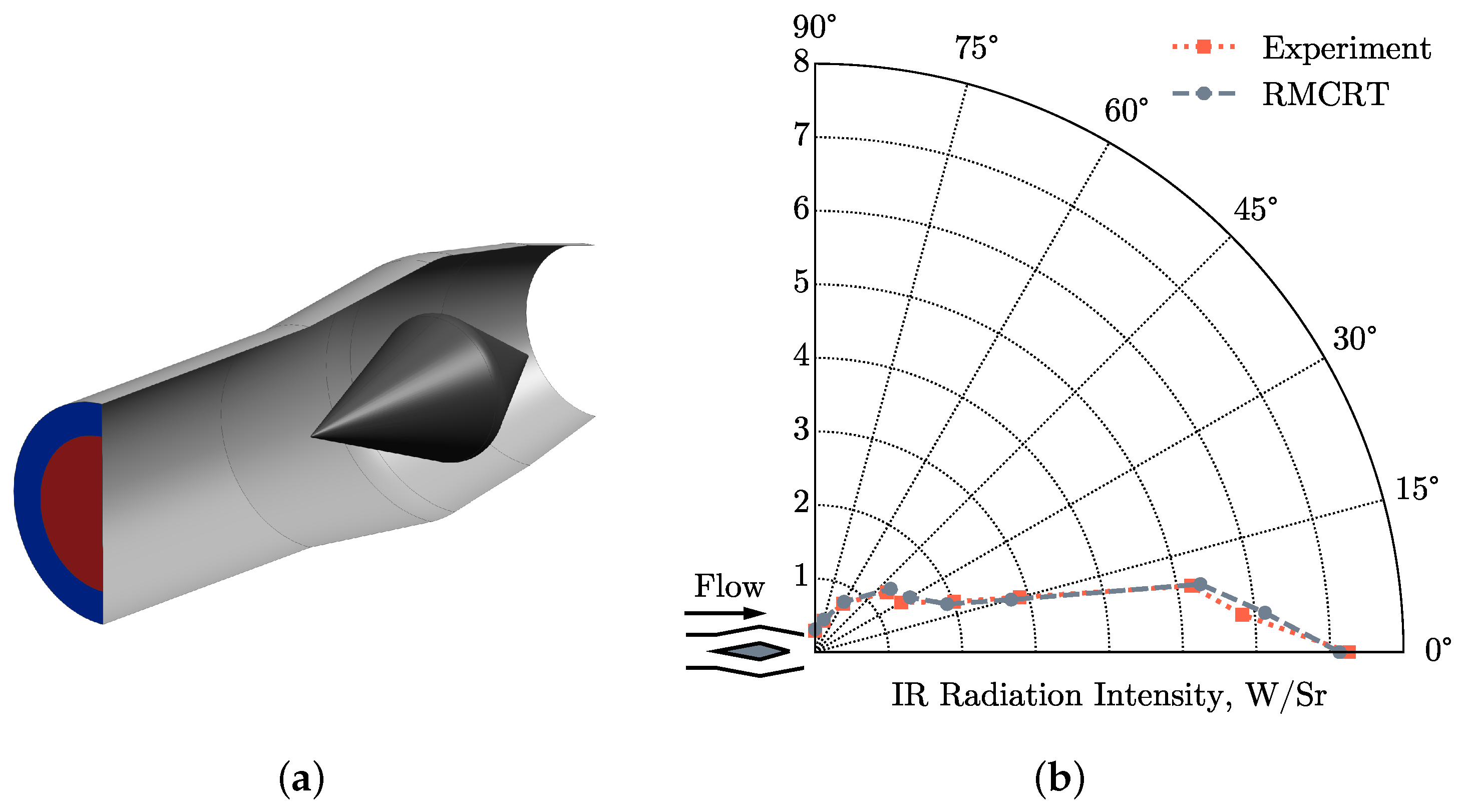
2.3. IR Radiation Calculation

The Reverse Monte Carlo ray tracing (RMCRT) method is adopted to calculate the infrared radiation of the serpentine nozzle. RMCRT is a stochastic method developed from the Monte Carlo Ray Tracing (MCRT) method, which can explicitly obtain solutions for the domain of interest without the need for the solution on the entire domain [24]. Therefore, RMCRT is much faster than MCRT when simulating the IR signature of a large scene with a complex shape, like the exhaust system of an aircraft. Based on the three-dimensional flow field data obtained via CFD simulation, inclusive of the temperature, pressure and component concentration of absorbing-emitting gas on the face and voxel, RMCRT can calculate the IR radiation characteristics of the target via ray tracing.
Generally, the IR sensor is positioned at a considerable distance from the aircraft, which significantly exceeds the aircraft’s characteristic length. This allows the aircraft to be treated as a point object emitting radiation. The radiant intensity emitted from the aircraft can be calculated as follows:
I = λ 1 λ 2 I λ d λ = λ 1 λ 2 E λ · R 2 d λ
where R is the distance from sensor to the target and λ 1 and λ 2 denote the boundaries of the detection waveband. E λ signifies the spectral irradiance directed toward the sensor, which can be determined by
E λ = Ω L λ ( s ) cos θ d Ω
Unlike the traditional and widely adopted discrete transfer method (DTM) [25,26], the RMCRT method does not discretize the incident solid angle. Instead, it randomly emits N rays within the stereo angle space, employs a probability density function to determine the final absorption location of the rays, and substitutes the actual radiation target with N statistically significant radiation sources. Consequently, the irradiance can be written as
E λ = i = 1 N L b λ ( i ) cos θ i N · Ω d
where L b λ ( i ) denotes the black body spectral radiance at the absorption point of the i-th random ray, where θ i is the angle between the ray and the normal direction of the detection surface. Since the sensor is far away from the target, cos θ i 1 , Equation (10) can be written as
I = λ 1 λ 2 A d i = 1 N L b λ ( i ) N · Ω d
In order to solve Equation (11) and calculate the radiance over a certain spectral band of wavelength, the most precise approach to this involves looping through the waveband of interest and calculating the radiance at each wave point. This requires calculating the contribution of each spectral line for all molecules in the atmospheric layer; this is called a line-by-line (LBL) calculation. Although it is acknowledged as the most accurate model for simulating thermal radiative transfer, the LBL calculation is exceptionally time-consuming due to the small spectral resolution [27]. To reduce the computation time, the statistic narrow band (SNB) model [28,29,30] is developed, wherein the spectral resolution is generally set between 5 and 50 cm 1 . Subsequently, Equation (11) can be simplified as
I = A d Δ λ N j = 1 M i = 1 N L b λ ( i , λ j )
where Δ λ is the spectral bandwidth and M denotes the number of discrete points in the waveband.
For the purpose of verifying the precision of the IR signature calculation code, the IR radiation characteristics of an experimental nozzle model proposed by Luo [31], as depicted in Figure 6 have been calculated and compared. The experimental nozzle is a scaled circular nozzle with a rear cone, making it suitable for comparison and validation. The simulation is conducted with parameters that mirror the experimental setup, where IR sensors are positioned 15 m from the nozzle exit in a circular arrangement. A comparison of experimental data and outcomes derived from the RMCRT is depicted in Figure 6. The experimental and simulated results only have a minor deviation at a few observation angles. For instance, at an observation angle of 20 , the maximum deviation of 7.46% can be observed. Despite these minor discrepancies, the overall agreement between the results acquired from the reversed Monte Carlo ray tracing method and the experimental data demonstrates the reliability of the RMCRT method in predicting the IR radiation signature of the elliptical double serpentine nozzle.

3. Optimization Method and Process

The comprehensive optimization of the aerodynamic characteristic and infrared radiation signature of the elliptical double serpentine nozzle is a multi-disciplinary and multi-objective optimization problem. In this section, the definition of Pareto concepts involved in multi-objective optimization is restated. Then, the general framework of Bayesian Optimization (BO) is presented. Moreover, the key driver of adaptive sampling in multi-objective Bayesian optimization, acquisition function, is introduced. Finally, the description of the optimization problem of this study and a detailed flowchart of the optimization process are presented.

3.1. Background on Multi-Objective Optimization

In general, there are conflicts between objectives in most multi-objective optimization tasks. In the Pareto method, we say a solution is Pareto-optimal if it is not possible to move from that point and improve at least one objective function without having a detrimental effect on any other objective function. Herein, we consider minimizing M 2 objective functions f m ( x ) : X R for m = 1 , 2 , , M where X R x d i m is the design space domain and x d i m is the number of design parameters. We say a solution f ( x ) = [ f ( 1 ) ( x ) , , f ( M ) ( x ) ] dominates another solution f ( x ) f ( x ) if f ( m ) ( x ) f ( m ) ( x ) for m = 1 , , M and m { 1 , , M } s . t . f ( m ) ( x ) > f ( m ) ( x ) . Then, the Pareto frontier can be defined as
P = f ( x ) : x X , x X s . t . f ( x ) f ( x )
and the set of Pareto-optimal designs can be denoted as
X = x : f ( x ) P

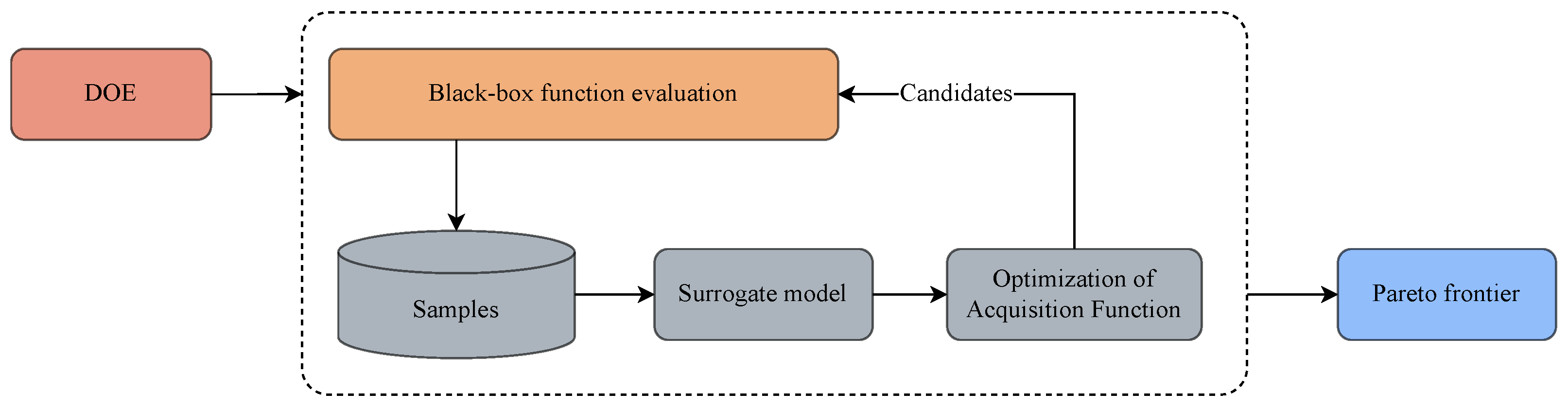
3.2. General Framework of Bayesian Optimization

During the past three decades, a large number of multi-objective optimization algorithms have been proposed, such as Evolutionary Algorithms (EA, e.g., NSGA-II) and Swarm Intelligence (SI, e.g., MOPSO), which show strong robustness to many problems. However, these algorithms require a large number of function evaluations [21,22], rendering them infeasible for solving the optimal problems with expensive-to-evaluate “black-box” functions (e.g., CFD simulation, hyper-parameter tuning in Machine Learning, etc.). The shape optimization of an elliptical double serpentine nozzle in this study involves numerous CFD simulations and infrared radiation calculations, which is suitable to be solved under multi-objective Bayesian optimization (MOBO). MOBO offers a sample-efficient method by generating the candidate solutions that best balance the predicted value and the uncertainty given all previous data [32].
The general framework of MOBO is shown in Figure 7. A probabilistic surrogate model is initially constructed once the initial sampling is completed by acquiring the corresponding objective values by implementing the black-box function. Typically, the surrogate is a Gaussian process regression (GPR), which is a flexible, non-parametric model known for its well-calibrated predictive uncertainty [33]. Subsequently, based on the posterior distribution P ( f | D ) over the true function values f provided by the GPR, the probabilistic surrogate model is updated via adaptive sampling, where the infill design point is determined by finding the maximum of the acquisition function x = arg max x X α ( x ) . This process is repeated for a fixed number of iterations, determined by the computational budget. Once the BO is finished, the probabilistic model is optimized to obtain the Pareto set of the optimization problem. The key to the success of BO is that the acquisition function is cheaper to evaluate than the black-box function [34]. In this study, the black-box function is the CFD simulation and IR calculation of the nozzle. Therefore, this can save a lot of expensive evaluations.

3.3. Expected Hyper-Volume Improvement

During each iteration of MOBO, an infill point is selected to enhance the surrogate model’s accuracy. This selection is based on optimizing a predifined acquisition function. The expected improvement (EI) criterion is a widely used acquisition function in Bayesian optimization, quantifying the potential improvement of the surrogate model at a specific input location. There are several variants of acquisition functions based on EI, such as Euclidean-based EI (EEI) [35], expected hypervolume improvement (EHVI) [36], ParEGO [37], and expected inverted penalty boundary intersection improvement (EIPBII) [38]. Among these variants, EHVI has been shown to perform well when applied to both artificial and aerodynamic problems, which makes it a highly promising MOBO method for multi-objective aerodynamic design optimization [39].
EHVI was first proposed by Emmerich [36] at 2006, and it is grounded in two fundamental concepts: hypervolume (HV) and hypervolume improvement (HVI). Both are utilized as general performance indicators in multi-objective optimization [40]. The hypervolume indicator of a finite approximate Pareto frontier P is the M-dimensional Lebesgue measure λ M of the space dominated by P and bounded from below by a reference point r :
HV ( P | r ) = λ M ( υ P r , υ )
where r , υ denotes the hyper-rectangle bounded by vertices r and υ . Typically, the reference point r is specified by the decision maker [41]. In this paper, the reference point was set to [1, 1] after the objective functions were normalized using the minimum and maximum values from the current experimental design. The HVI of a set of points P with reference to an existing approximate Pareto frontier P and reference point r is defined in Equation (16) and an illustration that depicts computing the HVI with new candidate f ( x ) is shown in Figure 8.
HVI ( P | P , r ) = HV ( P P | r ) HV ( P | r )
EHVI is the expected value of how much hypervolume improvement (HVI) can be obtained considering the current non-dominated solutions, the reference point, the Kriging prediction, and the Kriging estimation error. The analytical expression of EHVI can be formulated as
EHVI = E HVI f 1 ( x ) , f 2 ( x ) , , f M ( x ) = r 1 r 2 r M HVI f 1 ( x ) , f 2 ( x ) , , f M ( x ) × ϕ 1 ( f 1 ) ϕ 2 ( f 2 ) ϕ M ( f M ) d f 1 d f 2 d f M
where M is the number of objectives and ϕ ( f ) is the probability density function.
To verify the feasibility of the qEHVI acquisition function, we evaluate one synthetic benchmark, the Branin–Currin problem [42] ( d = 2 , M = 2 ), and one real-world benchmark, the Vehicle Safety problem [43] ( d = 5 , M = 3 ). The log hypervolume difference, which is defined as the difference between the hypervolume of the true Pareto front and the hypervolume of the approximate Pareto front based on the current observed data, is used as the evaluation criterion. The maximum hypervolume, reference point, search space and detailed problem definitions are presented in Appendix A. Four algorithms, including random search (Sobol), NSGA-II, and Bayesian optimization with qParEGO and qEHVI acquisition functions, respectively, are carried out on the two benchmark functions. In each run of the experiments, all algorithms are provided with 10 initial evaluations, and these initial inputs are shared across all algorithms. The experiments employed the Bayesian optimization model and acquisition function from the BoTorch framework [44], while the default implementations of the NSGA-II algorithm provided by the pymoo library [45].
Figure 9 illustrates the mean logHV difference over 20 runs. It can be seen that qEHVI outperforms the qParEGO, NSGA-II, and Sobol in terms of sequential optimization performance for the two optimization problems. Following the random initialization phase, the logHV difference of MOBO with qEHVI rapidly decreases. This indicates an increase in the HV and a closer proximity between the obtained Pareto frontier and the true frontier. The final experimental HV after 100 iterations and ideal HV for the two problems are shown in Table 5. It can be observed that qEHVI achieves a final HV that is very close to the theoretical HV. Compared to the Sobol, NSGA-II and qParEGO methods, qEHVI exhibits HV improvements of 38.84%, 2.69%, and 0.07% for the Branin–Currin problem, and 30.54%, 4.37%, and 0.264% for the vehicle safety problem, respectively. In addition, it is worth highlighting that the Bayesian algorithm demonstrates the lowest variance among the algorithms across multiple runs, which is particularly significant in practical applications where the expensive nature of the setting precludes the ability to perform multiple runs. This characteristic of the Bayesian algorithm makes it an attractive choice for the aerodynamic and stealth design, where computational resources are limited.
HV log _ diff = log ( HV max HV cur )

3.4. Formalizing the Problem

The aerodynamic performance of the elliptical double serpentine nozzle can be evaluated using the thrust coefficient C f , which is defined as the ratio of the actual thrust of the nozzle F x to the ideal thrust F i of the one-dimensional isentropic fully expanded flow, as shown in Equation (19). The closer the thrust coefficient is to 1, the smaller the flow loss inside the nozzle and the better aerodynamic performance of the nozzle.
C f = F x F i
and the F x and F i can be formulated as
F x = ρ e V e 2 + p e p b d A e
F i = m ˙ i 2 k k 1 R T i n 1 p b / p i n k 1 k , if NPR < 1.893 m ˙ i 2 k k + 1 R T i n + p i n / 1.893 p b A e , if NPR 1.893
where subscripts i n and e represent the inlet and exit sections of the nozzle, respectively. m ˙ i is the mass flow rate, which can be formulated as
m ˙ i = 2 k R ( k 1 ) p b / p i n 2 k p b / p i n k + 1 k p i n T A e , if NPR < 1.893 k R 2 k + 1 k + 1 k 1 p i n T A t , if NPR 1.893
In this study, the thrust coefficient of the serpentine nozzle C f is used as the objective function to evaluate the aerodynamic performance of the nozzle.
The objective function of the infrared radiation signature of the nozzle is a weighted summation of the infrared intensity mean values at different detection angles in different wavebands, as defined in Equation (23). The smaller the infrared intensity, the better the stealth performance of the elliptical double serpentine nozzle.
f i r = 1 2 N i = 1 N I i , M W I R + I i , L W I R
where N is the number of sensors, I is the infrared radiation intensity in the MWIR and LWIR band of the nozzle simulated by RMCRT. The primary objective of the elliptical double serpentine nozzle is to mitigate the IR signature by providing shielding for the high-temperature section and facilitating the thorough mixing of the high-temperature exhaust with the cool ambient air. However, this inevitably affects the aerodynamic performance of the engine exhaust system. Therefore, in order to search for the good infrared radiation suppression effect while taking into account the aerodynamic performance of the elliptical double serpentine nozzle, the following multi-objective optimization problem can be defined:
find : A R , L 1 min : C f , f I R s . t . A R 2 , 8 L 1 550 , 800   mm
where C f and f i r represent the thrust coefficient and infrared radiation objective function as defined in Equations (19) and (23), respectively. A R is the aspect ratio of the elliptical exit of the nozzle; L 1 is the length of the first serpentine section.

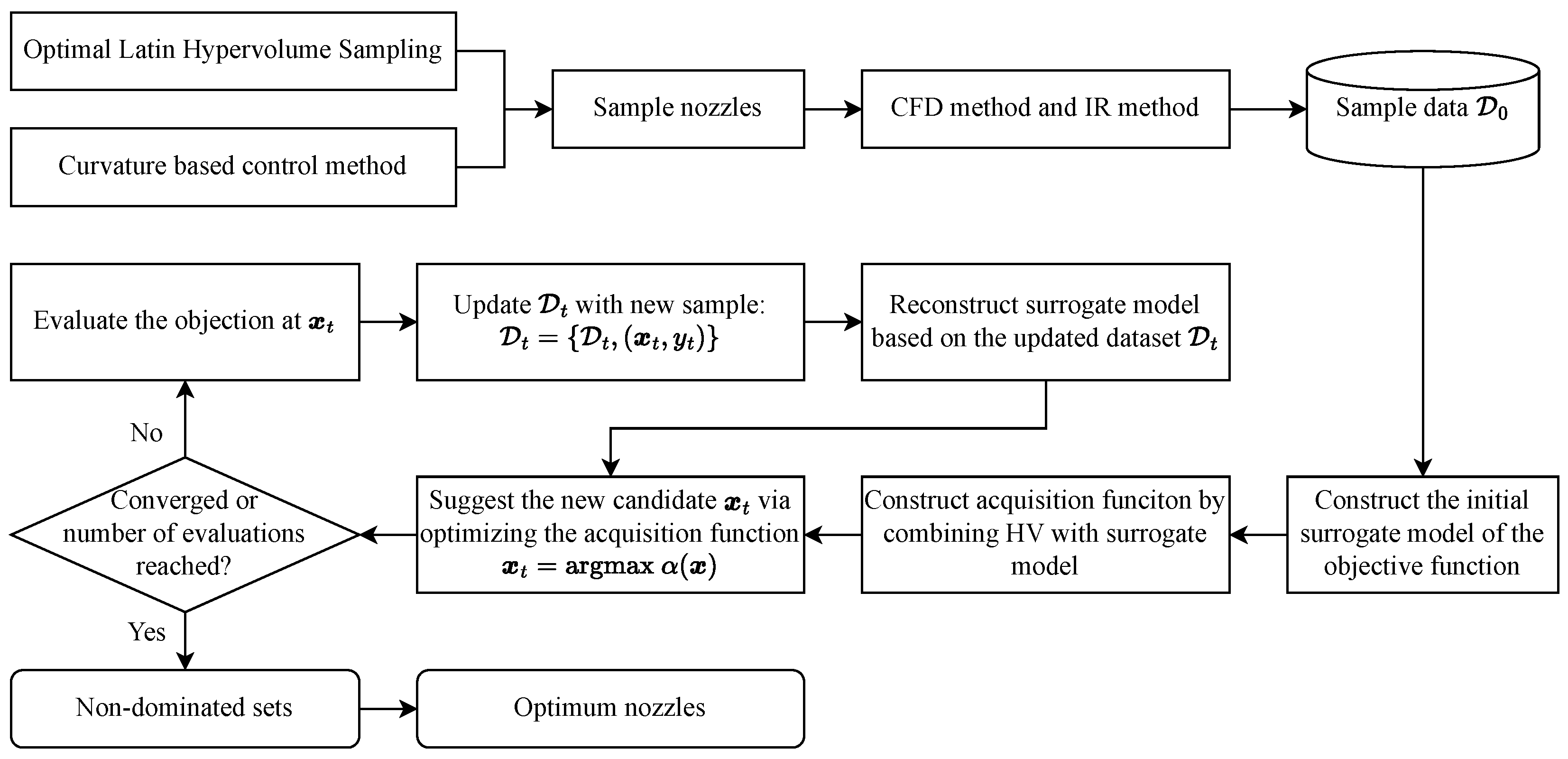
3.5. Optimization Procedure

Despite the existence of several space-filling techniques that are well suited for the design of experiment (DOE), Latin Hypercube Sampling (LHS) has attracted the most attention in recent years [46,47]. The Latin hypercube sampling (LHS) technique allows designers to freely select the number of design parameters and observations, rendering it an appealing option for optimization problems involving computationally expensive objective functions, such as aerodynamic simulations. In this study, an optimal Latin hypercube sampling (OLHS) is adopted to generate initial samples within the search space. This approach enhances LHS’s space-filling properties by utilizing a columnwise–pairwise algorithm to optimize the distribution of samples based on the S-optimality criterion [48,49].
The overall optimization procedure is shown in Figure 10. Firstly, 40 DOE points are generated as the initial samples in the search space. Subsequently, the aerodynamic characteristics and IR properties of 40 nozzles are then evaluated using the CFD and RMCRT method, respectively. Based on these data, a probabilistic surrogate model is constructed using the Kriging model to sequentially update the solution towards the Pareto frontier. At each iteration of MOBO, a new sample is generated according to the optimization of the acquisition function. This iterative process continues until the termination criteria are met. Finally, the non-dominated sets are obtained, from which the optimal serpentine nozzles are selected.

4. Results and Discussion

4.1. Optimization Details

Following the OLHS DOE process, a total of 40 samples are obtained, and both the aerodynamic characteristics and IR signature are simulated for each sample. The optimization objective functions, as defined in Equations (19) and (23), are subsequently computed, forming the initial dataset with which the probabilistic surrogate model is constructed. Prior to the optimization process, the Kriging surrogate model is assessed for its ability to generalize given data. The leave-one-out cross-validation (LOOCV) method is adopted to evaluate the Kriging surrogate model’s ability to predict objective values at unobserved locations. A detailed description of the LOOCV procedure can be found in [50].
The diagnostic plots from the LOOCV procedure for the C f and f i r surrogate models are presented on the left side of Figure 11, where values on the horizontal axis denote the exact results obtained through numerical simulation, and values on the vertical axis represent the prediction results from the Kriging model when the corresponding sample is omitted. A high-performing surrogate model would be characterized by samples located in close proximity to the diagonal line. In other words, the closer the samples are to the diagonal line, the better the surrogate model’s performance when it comes to capturing the underlying patterns and accurately predicting objective values at unobserved locations. It can be seen that the majority of observations cluster closely around the diagonal line, with only a few observations slightly deviating from the ideal location, suggesting that the model is capable of providing reliable predictions for both the thrust coefficient and IR signature of the elliptical double serpentine nozzle.
The right panel of Figure 11 depicts the distributions of the cross-validated residuals. The standardized residuals within a three-sigma range, denoted by the red shaded areas, correspond to a 99.7 % confidence interval for Gaussian processes like Kriging [51]. For the aerodynamic Kriging model, all samples fall within the desired interval, signifying the robust performance of the constructed surrogate model in predicting the thrust coefficient of the elliptical double serpentine nozzle. With respect to the IR surrogate model, three observations marginally exceed the desired boundaries. Nevertheless, apart from these anomalies, the majority of the residuals of the observations are distributed around the zero standard, indicating the model’s sufficiency in accurately predicting the IR signature of the serpentine nozzle.
In summation, the findings confirm the sufficient accuracy of the surrogate models constructed to predict both the aerodynamic performance and the IR characteristics of the elliptical double serpentine nozzle. These models, therefore, represent valuable tools for optimizing the nozzle’s design parameters and assessing their impact on the thrust coefficient and IR signature. This, in turn, contributes to the advancement of high-performance nozzle development for a range of applications.
In this study, due to the high computational cost of the CFD and IR simulations, only one new candidate is generated per iteration (q = 1) of Bayesian optimization. A straightforward initialization heuristic is employed to select 20 restart initial locations from a pool of 256 randomly generated points. A multi-start optimization of the qEHVI acquisition function is undertaken using LBFGS-B, with exact gradients computed via auto-differentiation powered by PyTorch.
Figure 12 presents the entire set of solutions projected into the infrared intensity and C f space. This includes both the initial samples and candidate observations accumulated throughout the iterations of Bayesian optimization. Since the multi-objective optimization problem defined above is a minimization problem, the x-axis denotes the negative C f . The brightness of the solutions’ color increases as the iterations progress in the BO. Such visualization of the results, preferably including interactive features, is particularly important to analyze in multi-objective optimization, as it can provide valuable insights for designers or decision-makers when evaluating different design option. It can be observed that the whole set of candidates obtained using the Bayesian algorithm appears to cluster in a more favorable area (the lower left corner of the Figure 12), which reflects the advantage of incorporating prior domain knowledge into Bayesian algorithms. This finding, together with the previous observations made on the respective performance of the algorithms in Figure 9, suggests that the Bayesian algorithm is capable of finding higher-quality trade-offs among the aerodynamic performance and infrared stealth performance of the elliptical double serpentine nozzle.

4.2. Comparison of Baseline and Optimal Nozzles

Furthermore, in order to highlight the characteristics of the elliptical double serpentine nozzle, the simulation results of an ordinary single serpentine nozzle with an elliptical exit are also presented for comparison. The geometric details of these models are shown in Figure 13. All four models have the same vertical offset. Compared to the Optimal-1 and Optimal-2 model, the first bend length of the Baseline model is smaller. Notably, the Optimal-2 model has a significantly larger aspect ratio than the others.
To highlight the superiority of each model, a thorough analysis of the aerodynamic and infrared radiation characteristics for each model, as presented in Figure 13, is conducted. The comparative simulation outcomes, detailed in Table 6, reveal that the Optimal-1 model exhibits enhanced aerodynamic characteristics and infrared stealth performance compared to the Baseline model. Specifically, the thrust coefficient C f improves by 0.27 % and the infrared radiation intensity f I R declines by 10.08 % . In contrast, the thrust coefficient of the Optimal-2 model has deteriorated due to its considerable aspect ratio. Nevertheless, this model achieves a more significant reduction in IR intensity than Optimal-1, with an average infrared intensity reduction of 18.12 % across MWIR and LWIR. This reduction is attributed to the larger aspect ratio of the nozzle exit, which better shields the engine’s hot components and enhances the blending of the hot plume with ambient air. The aerodynamic performance of the single serpentine nozzle improves by 0.61 % compared with the Baseline model. However, since the nozzle wall cannot fully block the hot part inside the nozzle, the mean IR intensity has been increased by 9.36 % . Furthermore, a substantial IR intensity peak is observed at ϕ = 80 , where the hot components such as the turbine section are directly exposed to the IR sensor, as depicted in Figure 14. It is noteworthy that while the double serpentine nozzle can detrimentally impact the aerodynamic performance of the nozzle flow field, the complete shielding of the high-temperature part and hot plume inside the nozzle can effectively reduce the infrared radiation signature. The data presented in Table 6 suggest that there is a trade-off between aerodynamic performance and infrared stealth performance for the elliptical double serpentine nozzle. By optimizing the nozzle shape, it is feasible to achieve an overall performance enhancement relative to the Baseline model.
The z-axis time-averaged vorticity distribution across different cross sections of each model is presented in Figure 15, allowing us to analyze the internal flow field within the nozzle. As illustrated, the presence of the central cone results in an augmented rotational velocity of the time-averaged vorticity as the radius of the cone decreases, in accordance with the law of conservation of angular momentum. Consequently, a concentrated vortex is formed downstream of the central cone. The vortex generated by the central cone then accelerates the expansion of the core flow, thereby enhancing the mixing of the core and bypass flows. Furthermore, the shear effect between the core and bypass flows induces a pronounced streamwise vortex within the elliptical nozzle. The intensity of these streamwise vortexes is notably higher in the double serpentine nozzle compared to the single serpentine nozzle due to its curved geometric configuration. In the case of the Baseline model, where the length of the first bend is shorter than the other two double serpentine models, a substantial flow deflection occurs within this section. Consequently, two distinct streamwise vortexes develop within the first bend and persist until they reach the exit of the nozzle. In contrast, the Optimal-1 and Optimal-2 models, which have longer first bend sections, develop two pairs of streamwise vortexes in the second bend of the nozzle. As a result, the flow at the nozzle exit becomes more uniform, and the aerodynamic performance of the nozzle improves.
The IR radiation intensity distributions of the single serpentine nozzle and Baseline model are illustrated in Figure 14. The polar lines on the left represent the total IR radiation intensity, which is the summation of the IR radiation of the solid wall of the nozzle (right) and the IR radiation of gas (middle). The IR radiation intensity of the wall received by the detector is the radiation emitted from the solid wall boundaries of the nozzle, including the nozzle wall, the nozzle mixer, and the nozzle central cone, which has been attenuated by the gas. The IR radiation intensity from the nozzle wall is determined by the visibility of the nozzle’s hot part and the wall itself to the detector. Given that the IR radiative power E is significantly sensitive to the temperature ( E = σ T 4 ), the temperature distribution of the visible wall is the primary determinant of the nozzle’s IR radiation characteristic. This sensitivity results in a noticeable peak in the IR intensity for the single serpentine nozzle, as the single serpentine nozzle does not fully block the hot part inside the nozzle.
The primary effect of the double serpentine nozzle is to shield the high-temperature components inside the nozzle, such as the nozzle central cone and turbo section. The IR intensity of the Baseline model remains relatively low at most detection angles, with the exception of when the detection angle θ falls within the range of 90 140 . This exception is attributable to the hot streak located at the upper nozzle wall, a phenomenon which will be further explained in the following discussions. The hot exhausted gas produced by the engine can be divided into two parts: gas inside the nozzle exit and gas outside the nozzle exit. The single serpentine configuration would require a significant offset for complete internal component shielding, a requirement that presents substantial design and integration challenges, as noted by Cheng et al. [1].
The top panel of Figure 16 displays the temperature contours across the cross sections of the Baseline model, Optimal-1 and Optimal-2 models. As the flow develops, the high-temperature core flow consistently mixes with the bypass flow, gradually reducing the temperature of the core flow. The wall curvature and the transition from circular to elliptical induce the formation of two vortices at the sides of the nozzle. This leads to a distinct temperature distribution pattern at the elliptical exit of the elliptical double serpentine nozzle. Notably, the non-uniformity at the nozzle exit of Optimal model is appreciably diminished.
The temperature distributions of each model’s nozzle wall are depicted in the bottom panel of Figure 16. Notably, a band-like distribution of localized high-temperature regions, also known as a “hot streak”, is evident on the upper wall of the nozzle. In the Baseline model, this hot streak originates at the second bend of the nozzle and extends into the straight sections. Conversely, the hot streak in the Optimal models is primarily confined to the straight sections. In comparison to the Baseline model, not only is the area of these hot streaks smaller, but their temperature is also significantly reduced. The temperature manifests a gradual decrease from the central region towards the side in the cross-sectional direction of the nozzle.
Figure 17 depicts the angular distribution of the infrared intensity of the elliptical double serpentine nozzle on the pitch detection plane. The top panel represents the infrared radiation in the middle-wavelength band (3–5 µm), while the bottom panel corresponds to the infrared radiation in the long-wavelength band (8–14 µm). There is a clear distinction between the distribution patterns of the MWIR intensity and those in the LWIR. In the MWIR range, the infrared radiation is dominated by the hot plume of the nozzle, while the solid radiation accounts for a relatively small part. As the detector shifts away from the aft end of the nozzle ( θ = 90 ), the MWIR intensity gradually increases, as demonstrated in Figure 17b. This rise is attributable to the increasing projected area of the hot plume on the detector focal plane as the detector moves away, thereby increasing the infrared intensity. When the detector is positioned directly above ( θ = 0 ) or below ( θ = 180 ) the nozzle, only the infrared radiation emitted from the plume is accessible to the detector.
It can be observed that the hot streak has a significant impact on the infrared radiation characteristic of the three elliptical double serpentine nozzles. The peak solid infrared radiation within both the MWIR (Figure 17c) and LWIR (Figure 17f) occurs at a detection angle around 110 in the vertical detection plane. This is because the infrared radiation emitted from the hot streak can be received by the IR sensors, and the projected area is maximized at this detection angle. In addition, the solid LWIR intensity is larger than the MWIR intensity, which can be explained by Wein’s displacement law. Given the area and temperature of the hot streak in Optimal-1 and Optimal-2 model, these models exhibit a noticeable decrease in solid infrared radiation, which is consistent with the temperature distribution pattern of the hot streak shown in Figure 16.
Observing Figure 17b, it is noticeable that in the middle waveband, the gas radiation of the Optimal-2 model (blue line) is smaller than the gas radiation of the Optimal-1 model (gray line) at most detection angles. This reduction is attributed to the larger exit aspect ratio of the Optimal-2 model, which enhances the mixing of the hot exhaust flame with ambient cool air, thereby reducing the temperature of the tail flame core area (as shown in Figure 18) and consequently decreasing its radiation energy. On the other hand, the larger aspect ratio of Optimal-2 model results in a somewhat stronger hot spot in the Optimal-2 model compared to the Optimal-1 model. Figure 17f reveals that the solid radiation of the Optimal-2 model is slightly higher than that of the Optimal-1 model. Simultaneously, the stronger vortex caused by the larger aspect ratio in the Optimal-2 nozzle leads to a minor reduction in the aerodynamic characteristics compared to the Baseline model and the Optimal-1 model. Moreover, in our study, we found that for the serpentine nozzle, due to the complete shielding of high-temperature components by the double S-bend design of the nozzle, the solid radiation emanates predominantly from the nozzle wall. At most detection angles, the radiation from other components is virtually negligible. This finding underscores the effectiveness of the double S-bend nozzle in protecting against infrared radiation from the internal high-temperature sections.
Figure 18 reveals the infrared radiation intensity images within the MWIR and LWIR bands for different models. These images provide an intuitive view of the variations in high-temperature areas of different nozzles. The left side of Figure 18 presents the infrared radiation intensity images observed from above the nozzle ( θ = 90 , ϕ = 0 ). It is evident that there is an alternation between high- and low-temperature zones at the nozzle exit generated by shock waves. The Optimal-1 model exhibits a high-temperature tail flame length nearly identical to that of the Baseline model. However, the exhaust flame length of the Optimal-2 model is noticeably shorter, with bifurcation evident in the plume. This is because the Optimal-2 model’s nozzle exit has a larger aspect ratio ( A R = 7.8 ), which enhances the mixing of the plume with the ambient cold air, resulting in the strong 3-D effect of the fluid. Thereby, the high-temperature core length of Optimal-2 is shorter than that of the other two models. Correspondingly, the IR radiation intensity of gas is also reduced, as shown in Figure 17. The right side of Figure 18 features the infrared radiation intensity images from the rear perspective ( θ = 90 , ϕ = 90 ). The Baseline model exhibits a significantly higher hot streak intensity compared to the Optimal-1 and Optimal-2 models, resulting in a notably dimmer appearance for the latter. This observation corroborates the quantitative findings presented earlier in Figure 17 and Table 6.

5. Conclusions

In this paper, a state-of-the-art multi-objective Bayesian optimization algorithm was adapted to an aerodynamic and infrared stealth optimization problem for the elliptical double serpentine nozzle. Based on the curvature control method, a series of nozzles were designed to perform the Bayesian optimization. The Pareto frontier was finally obtained and two non-dominated solutions on the PF were selected to obtain the optimal model. A detailed comparison of the characteristics of these two models with the Baseline model and one single serpentine nozzle was carried out. The main conclusions can be drawn as follows:
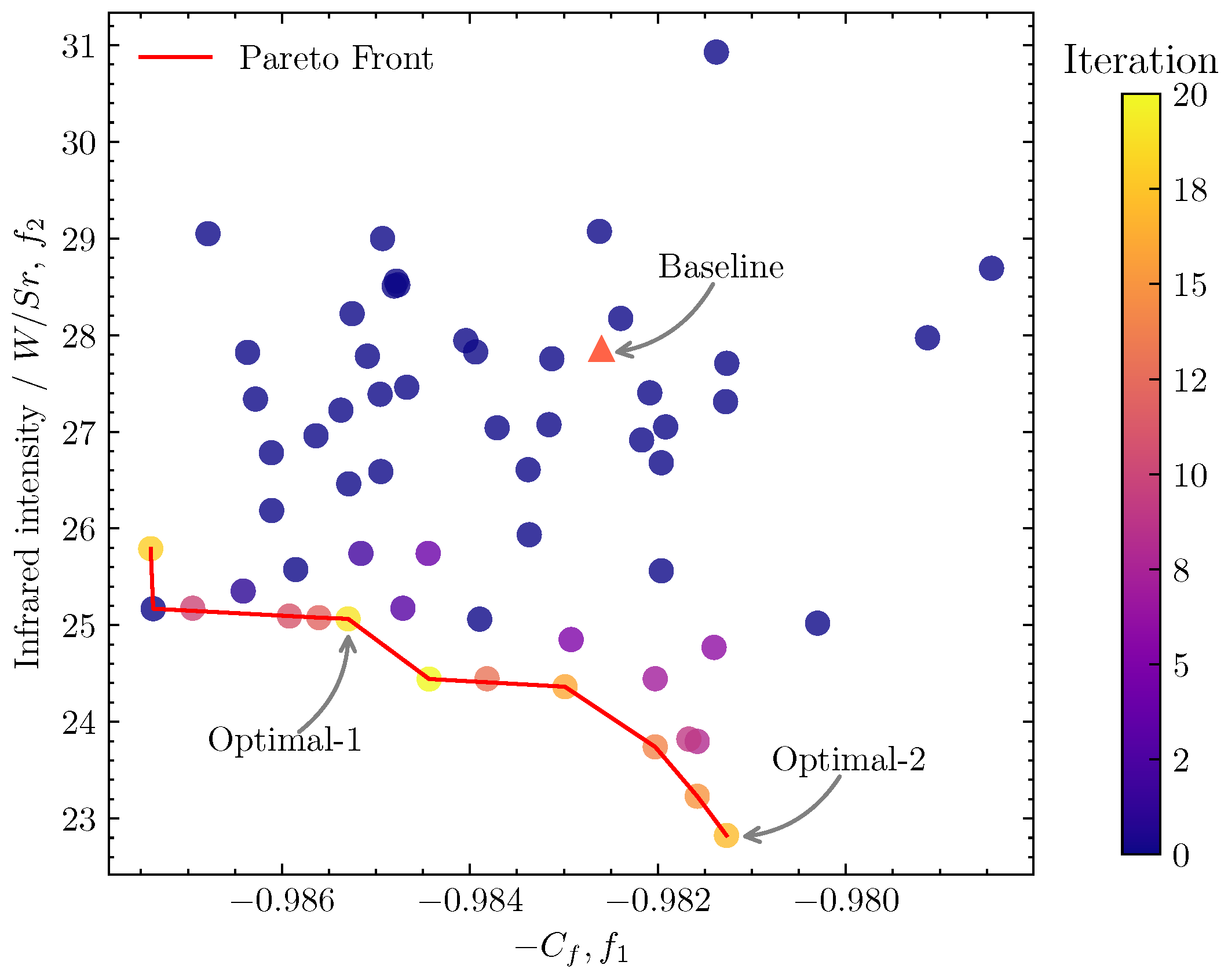
  • The length of the first bend and the aspect ratio of the elliptical double serpentine nozzle have an important influence on the performance of the nozzle. Notably, the Optimal-1 model demonstrated enhanced infrared radiation and aerodynamic performance following the optimization, with a 10.08 % decrease in infrared radiation intensity and a 0.27 % improvement in the thrust coefficient.
  • The Optimal-2 model, with a larger aspect ratio, showed an impressive improvement in the infrared radiation performance, demonstrated by an 18.12 % reduction in infrared radiation intensity. However, the larger transition from circular inlet to elliptical exit also deteriorated the flow field of the Optimal-2 model, while the thrust coefficient decreased by 0.14 % .
  • The optimization framework introduced in this paper effectively tackles the complex multi-objective optimization problems of the elliptical double serpentine nozzle. This framework not only provides reliable technical guidance for future research, but is also a promising approach to complex and costly optimization challenges in aircraft design, including the improvement of aerodynamic, radar, and infrared stealth capabilities.

Author Contributions

Conceptualization, S.Z. and Q.Y.; methodology, S.Z.; software, S.Z. and R.W.; validation, S.Z.; formal analysis, Q.Y.; investigation, S.Z.; resources, S.Z. and Q.Y.; data curation, S.Z.; writing—original draft preparation, S.Z. and R.W.; writing—review and editing, Q.Y. and X.W.; visualization, S.Z. and X.W.; supervision, Q.Y. All authors have read and agreed to the published version of the manuscript.

Funding

This work was supported by the Natural Science Basic Research Program of Shaanxi (Program No. 2022JQ-052).

Data Availability Statement

Data are contained within the article.

Conflicts of Interest

The authors declare no conflicts of interest.

Nomenclature

Abbreviations
ARAspect Ratio.
BOBayesian Optimization.
CFDComputational Fluid Dynamic.
DOEDesign of Experiment.
DTMDiscrete Transfer Method.
EAEvolutionary Algorithms.
EHVIExpected Hypervolume Improvement.
EIExpected Improvement.
HVHypervolume.
IRInfra-Red.
LBLLine by Line.
LHSLatin Hypercube Sampling.
LOOCVLeave One Out Cross Validation.
LWIRLong Wavelength Infrared.
MOBOMulti-Objective Bayesian Optimization.
MWIRMiddle Wavelength Infrared.
NSGANon-dominated Sorting Genetic Algorithm.
OLHOptimal Latin Hypercube.
RMCRTReversed Monte Carlo Ray Tracing.
PFPareto Frontier.
SNBStatistic Narrow Band.
UCAVUnmanned Combat Aerial Vehicle.
Others
P Approximated Pareto front.
p b Back pressure.
mDimension of an objective space.
IInfrared intensity.
m ˙ i Mass flow rate of nozzle.
μ Mean value of predictive distribution.
ϕ Pitch detection angle.
σ Standard deviation of predictive distribution.
C f Thrust coefficient of nozzle.
λ Wavelength.
θ Yaw detection angle.

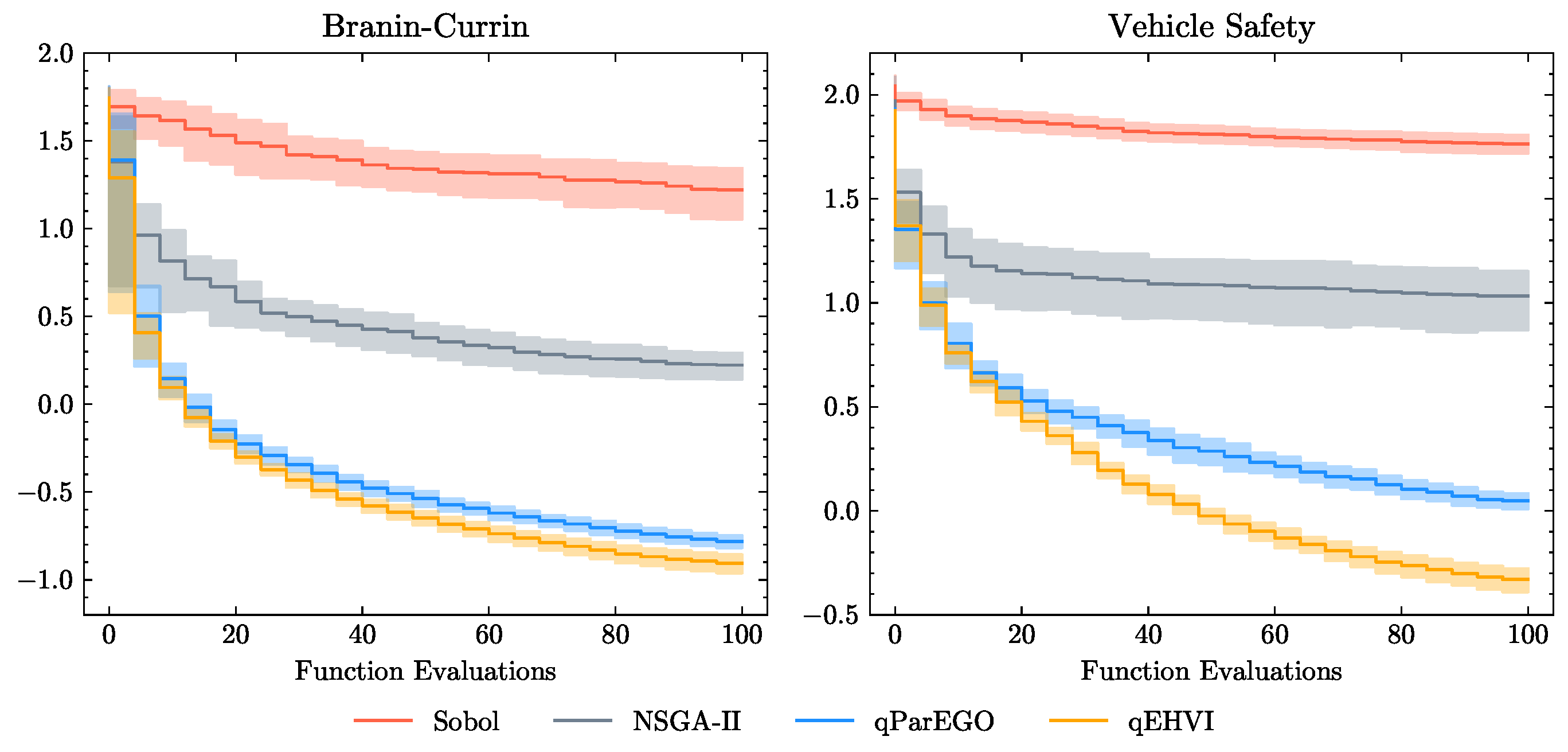
Appendix A. Benchmark Problems

Appendix A.1. Branin–Currin Function

f 1 ( x 1 ) = ( x 2 5.1 4 π 2 x 1 2 + 5 π x 1 r ) 2 + 10 ( 1 1 8 π ) cos ( x 1 ) + 10 f 2 ( x 2 ) = 1 exp 1 ( 2 x 2 ) 2300 x 1 3 + 1900 x 1 2 + 2092 x 1 + 60 100 x 1 3 + 500 x 1 2 + 4 x 1 + 20
where x 1 , x 2 [ 0 , 1 ] , x 1 = 15 x 1 5 , and x 2 = 15 x 2 . Reference point is [18.0, 6.0]. Max HV = 59.36.

Appendix A.2. Vehicle Safety Function

Vehicle crash safety is an important consideration in the structural design of cars. The goal is to minimize: (1) the mass of the vehicle; (2) the collision acceleration in a full frontal crash; and (3) the toe-board intrusion—a measure of the most extreme mechanical damage to the vehicle in an off-frontal collision. For this problem, the surrogate model we used are given by [43]:
f 1 ( x ) = 1640.2823 + 2.3573285 x 1 + 2.3220035 x 2 + 4.5688768 x 3 + 7.7213633 x 4 + 4.4559504 x 5 f 2 ( x ) = 6.5856 + 1.15 x 1 1.0427 x 2 + 0.9738 x 3 + 0.8364 x 4 0.3695 x 1 x 4 + 0.0861 x 1 x 5 + 0.3628 x 2 x 4 + 0.1106 x 1 2 0.3437 x 3 2 + 0.1764 x 4 2 f 3 ( x ) = 0.0551 + 0.0181 x 1 + 0.1024 x 2 + 0.0421 x 3 0.0073 x 1 x 2 + 0.024 x 2 x 3 0.0118 x 2 x 4 0.0204 x 3 x 4 0.008 x 3 x 5 0.0241 x 2 2 + 0.0109 x 4 2
where x [ 1 , 3 ] 5 . Reference point is [1864.72022, 11.81993945, 0.2903999384]. Max HV = 246.82.

References

  1. Cheng, W.; Wang, Z.; Zhou, L.; Sun, X.; Shi, J. Influences of shield ratio on the infrared signature of serpentine nozzle. Aerosp. Sci. Technol. 2017, 71, 299–311. [Google Scholar] [CrossRef]
  2. Nangia, R.; Ghoreyshi, M.; van Rooij, M.P.; Cummings, R.M. Aerodynamic design assessment and comparisons of the MULDICON UCAV concept. Aerosp. Sci. Technol. 2019, 93, 105321. [Google Scholar] [CrossRef]
  3. Li, M.; Bai, J.; Li, L.; Meng, X.; Liu, Q.; Chen, B. A gradient-based aero-stealth optimization design method for flying wing aircraft. Aerosp. Sci. Technol. 2019, 92, 156–169. [Google Scholar] [CrossRef]
  4. Wang, B.; Cong, W.; Wang, C.; Yang, Y.; Huang, J. Infrared radiation characteristics calculation and infrared stealth effect analysis of stealth fighter. Trans. Beijing Inst. Technol. 2019, 39, 365–371. [Google Scholar]
  5. Rao, A.N.; Kushari, A.; Jaiswal, G.K. Effect of nozzle geometry on flowfield for high subsonic jets. J. Propuls. Power 2018, 34, 1596–1608. [Google Scholar] [CrossRef]
  6. Feng, N. Development and application of stealth technique. Int. Technol. 2012, 119, 86–102. [Google Scholar]
  7. Born, G.A.; Roberts, T.A.; Boor, P.M. Infrared Suppression Exhaust Duct System for a Turboprop Propulsion System for an Aircraft. U.S. Patent 5,699,662, 23 December 1997. [Google Scholar]
  8. Johansson, M. FOT25 2003–2005 Propulsion Integration Final Report; Report No. FOI; Swedish Defence Research Agency (FOI): Stockholm, Sweden, 2006.
  9. Ho, C.M.; Gutmark, E. Vortex induction and mass entrainment in a small-aspect-ratio elliptic jet. J. Fluid Mech. 1987, 179, 383–405. [Google Scholar] [CrossRef]
  10. Miller, R.; Madnia, C.; Givi, P. Numerical simulation of non-circular jets. Comput. Fluids 1995, 24, 1–25. [Google Scholar] [CrossRef]
  11. Baranwal, N.; Mahulikar, S.P. Review of Infrared signature suppression systems using optical blocking method. Def. Technol. 2019, 15, 432–439. [Google Scholar] [CrossRef]
  12. Liu, C.; Ji, H.; Huang, W.; Yang, F. Numerical simulation on infrared radiation characteristics of serpentine 2-D nozzle. J. Aerosp. Power 2013, 28, 1482–1488. [Google Scholar]
  13. An, C.; Kang, D.; Baek, S.; Myong, R.; Kim, W.; Choi, S. Analysis of plume infrared signatures of S-shaped nozzle configurations of aerial vehicle. J. Aircr. 2016, 53, 1768–1778. [Google Scholar] [CrossRef]
  14. Rajkumar, P.; Chandra Sekar, T.; Kushari, A.; Mody, B.; Uthup, B. Flow characterization for a shallow single serpentine nozzle with aft deck. J. Propuls. Power 2017, 33, 1130–1139. [Google Scholar] [CrossRef]
  15. Crowe, D.S.; Martin, C.L. Effect of geometry on exit temperature from serpentine exhaust nozzles. In Proceedings of the 53rd AIAA Aerospace Sciences Meeting, Kissimmee, FL, USA, 5–9 January 2015; p. 1670. [Google Scholar]
  16. Crowe, D.S.; Martin, C.L. Hot streak characterization in serpentine exhaust nozzles. In Proceedings of the 52nd AIAA/SAE/ASEE Joint Propulsion Conference, Salt Lake City, UT, USA, 25–27 July 2016; p. 4502. [Google Scholar]
  17. Crowe, D.S.; Martin, C.L., Jr. Hot streak characterization of high-performance double-serpentine exhaust nozzles at design conditions. J. Propuls. Power 2019, 35, 501–511. [Google Scholar] [CrossRef]
  18. Cheng, W.; Wang, Z.; Zhou, L.; Shi, J.; Sun, X. Infrared signature of serpentine nozzle with engine swirl. Aerosp. Sci. Technol. 2019, 86, 794–804. [Google Scholar] [CrossRef]
  19. Singh, L.; Singh, S.; Sinha, S. Effect of Reynolds number and slot guidance on passive infrared suppression device. Aerosp. Sci. Technol. 2020, 99, 105732. [Google Scholar] [CrossRef]
  20. Liu, J.; Yue, H.; Lin, J.; Zhang, Y. A simulation method of aircraft infrared signature measurement with subscale models. Procedia Comput. Sci. 2019, 147, 2–16. [Google Scholar] [CrossRef]
  21. Deb, K.; Pratap, A.; Agarwal, S.; Meyarivan, T. A fast and elitist multiobjective genetic algorithm: NSGA-II. IEEE Trans. Evol. Comput. 2002, 6, 182–197. [Google Scholar] [CrossRef]
  22. Coello, C.C.; Lechuga, M.S. MOPSO: A proposal for multiple objective particle swarm optimization. In Proceedings of the 2002 Congress on Evolutionary Computation. CEC’02 (Cat. No. 02TH8600), Honolulu, HI, USA, 12–17 May 2002; Volume 2, pp. 1051–1056. [Google Scholar]
  23. Lee, C.; Boedicker, C. Subsonic diffuser design and performance for advanced fighter aircraft. In Proceedings of the Aircraft Design Systems and Operations Meeting, Colorado Springs, CO, USA, 14–16 October 1985; p. 3073. [Google Scholar]
  24. Sun, X.; Smith, P.J. A Parametric Case Study in Radiative Heat Transfer Using the Reverse Monte-Carlo Ray-Tracing with Full-Spectrum k-Distribution Method. J. Heat Transf. 2009, 132, 024501. [Google Scholar] [CrossRef]
  25. Lockwood, F.; Shah, N. A new radiation solution method for incorporation in general combustion prediction procedures. Symp. Int. Combust. 1981, 18, 1405–1414. [Google Scholar] [CrossRef]
  26. Versteeg, H.K.; Henson, J.C.; Malalasekera, W. Spatial discretization errors in the heat flux integral of the discrete transfer method. Numer. Heat Transf. Part B Fundam. 2000, 38, 333–352. [Google Scholar]
  27. Schenker, G.N.; Keller, B. Line-by-line calculations of the absorption of infrared radiation by water vapor in a box-shaped enclosure filled with humid air. Int. J. Heat Mass Transf. 1995, 38, 3127–3134. [Google Scholar] [CrossRef]
  28. Malkmus, W. Random Lorentz Band Model with Exponential-Tailed S—1 Line-Intensity Distribution Function. J. Opt. Soc. Am. 1967, 57, 323–329. [Google Scholar] [CrossRef]
  29. Young, S.J. Nonisothermal band model theory. J. Quant. Spectrosc. Radiat. Transf. 1977, 18, 1–28. [Google Scholar] [CrossRef]
  30. Zheng, S.; Yang, Y.; Zhou, H. The effect of different HITRAN databases on the accuracy of the SNB and SNBCK calculations. Int. J. Heat Mass Transf. 2019, 129, 1232–1241. [Google Scholar] [CrossRef]
  31. Luo, M. Investigation of Infrared Stealth Technology of the Exhaust System for Unmanned Aerial Vehicle. Ph.D. Thesis, Nanjing University of Aeronautics and Astronautics, Nanjing, China, 2006. [Google Scholar]
  32. Shahriari, B.; Swersky, K.; Wang, Z.; Adams, R.P.; de Freitas, N. Taking the Human Out of the Loop: A Review of Bayesian Optimization. Proc. IEEE 2016, 104, 148–175. [Google Scholar] [CrossRef]
  33. Seeger, M. Gaussian processes for machine learning. Int. J. Neural Syst. 2004, 14, 69–106. [Google Scholar] [CrossRef] [PubMed]
  34. Fernández-Sánchez, D.; Garrido-Merchán, E.C.; Hernández-Lobato, D. Improved max-value entropy search for multi-objective bayesian optimization with constraints. Neurocomputing 2023, 546, 126290. [Google Scholar] [CrossRef]
  35. Keane, A.J. Statistical improvement criteria for use in multiobjective design optimization. AIAA J. 2006, 44, 879–891. [Google Scholar] [CrossRef]
  36. Emmerich, M.T.; Giannakoglou, K.C.; Naujoks, B. Single-and multiobjective evolutionary optimization assisted by Gaussian random field metamodels. IEEE Trans. Evol. Comput. 2006, 10, 421–439. [Google Scholar] [CrossRef]
  37. Knowles, J. ParEGO: A hybrid algorithm with on-line landscape approximation for expensive multiobjective optimization problems. IEEE Trans. Evol. Comput. 2006, 10, 50–66. [Google Scholar] [CrossRef]
  38. Namura, N.; Shimoyama, K.; Obayashi, S. Expected improvement of penalty-based boundary intersection for expensive multiobjective optimization. IEEE Trans. Evol. Comput. 2017, 21, 898–913. [Google Scholar] [CrossRef]
  39. Zuhal, L.R.; Palar, P.S.; Shimoyama, K. A comparative study of multi-objective expected improvement for aerodynamic design. Aerosp. Sci. Technol. 2019, 91, 548–560. [Google Scholar] [CrossRef]
  40. Yang, K.; Emmerich, M.; Deutz, A.; Bäck, T. Efficient computation of expected hypervolume improvement using box decomposition algorithms. J. Glob. Optim. 2019, 75, 3–34. [Google Scholar] [CrossRef]
  41. Yang, K.; Emmerich, M.; Deutz, A.; Bäck, T. Multi-objective Bayesian global optimization using expected hypervolume improvement gradient. Swarm Evol. Comput. 2019, 44, 945–956. [Google Scholar] [CrossRef]
  42. Belakaria, S.; Deshwal, A.; Doppa, J.R. Max-value entropy search for multi-objective Bayesian optimization. Adv. Neural Inf. Process. Syst. 2019, 32. [Google Scholar]
  43. Tanabe, R.; Ishibuchi, H. An easy-to-use real-world multi-objective optimization problem suite. Appl. Soft Comput. 2020, 89, 106078. [Google Scholar] [CrossRef]
  44. Balandat, M.; Karrer, B.; Jiang, D.; Daulton, S.; Letham, B.; Wilson, A.G.; Bakshy, E. BoTorch: A framework for efficient Monte-Carlo Bayesian optimization. Adv. Neural Inf. Process. Syst. 2020, 33, 21524–21538. [Google Scholar]
  45. Blank, J.; Deb, K. pymoo: Multi-Objective Optimization in Python. IEEE Access 2020, 8, 89497–89509. [Google Scholar] [CrossRef]
  46. Liu, H.; Ong, Y.S.; Cai, J. A survey of adaptive sampling for global metamodeling in support of simulation-based complex engineering design. Struct. Multidiscip. Optim. 2018, 57, 393–416. [Google Scholar] [CrossRef]
  47. Viana, F.A. Things you wanted to know about the Latin hypercube design and were afraid to ask. In Proceedings of the 10th World Congress on Structural and Multidisciplinary Optimization, Orlando, FL, USA, 19–24 May 2013; Volume 19. [Google Scholar]
  48. Joseph, V.R. Space-filling designs for computer experiments: A review. Qual. Eng. 2016, 28, 28–35. [Google Scholar] [CrossRef]
  49. Santner, T.J.; Williams, B.J.; Notz, W.I.; Santner, T.J.; Williams, B.J.; Notz, W.I. Space-filling designs for computer experiments. In The Design and Analysis of Computer Experiments; STAT Center of Excellence: Dayton, OH, USA, 2018; pp. 145–200. [Google Scholar]
  50. Drezek, P.S.; Kubacki, S.; Zoltak, J. Kriging-Based Framework Applied to a Multi-Point, Multi-Objective Engine Air-Intake Duct Aerodynamic Optimization Problem. Aerospace 2023, 10, 266. [Google Scholar] [CrossRef]
  51. Jones, D.R.; Schonlau, M.; Welch, W.J. Efficient global optimization of expensive black-box functions. J. Glob. Optim. 1998, 13, 455–492. [Google Scholar] [CrossRef]
Figure 1. Schematic diagram of the exhaust system under examination. The exhaust system comprises three main components: the mixing chamber, the double serpentine nozzle, and the straight section. For detailed geometrical parameters, refer to Table 1.
Aerospace 11 00048 g001
Figure 2. Different distributions of area, curvature, and centerline of Lee curve [23].
Aerospace 11 00048 g002
Figure 3. Computational grid of the elliptical double serpentine nozzle. (a) global computational grid. (b) nozzle grid.
Aerospace 11 00048 g003
Figure 4. Arrangement of infrared sensors. IR sensors are strategically positioned on the x O y and y O z planes in a circumferential pattern. They are spaced at 2-degree intervals around the circumference, with each sensor located 5 km from the nozzle.
Aerospace 11 00048 g004
Figure 5. Grid sensitivity analysis across four distinct grid sizes. To balance computational load with precision, the grid comprising 4.4 million cells was selected.
Aerospace 11 00048 g005
Figure 6. Verification of RMCRT. Panel (a) Model of the experimental nozzle depicts a scaled model with a rear cone proposed by Luo [31]. Panel (b) Comparison of the simulation result and experimental data for IR validation, validates the accuracy of the RMCRT method in simulating the infrared radiation signature of the nozzle.
Aerospace 11 00048 g006
Figure 7. General framework of multi-objective Bayesian optimization.
Aerospace 11 00048 g007
Figure 8. The illustration of computing the hypervolume improvement with infill point f ( x ) when there are two objectives. The current Pareto frontier P is given by the green points and the red area is the hypervolume surrounded by the P and given reference point r . The white rectangles S 1 , , S K represent a disjoint box decomposition of the non-dominated space, which can be utilized to compute the hypervolume improvement efficiently.
Aerospace 11 00048 g008
Figure 9. A comparison of different algorithms used for synthetic test function (left) and a real-world problem (right). The hypervolume indicator is shown with regard to the number of function evaluations. Every experiment has a batch size of 4 and 25 iterations in total. The means and one standard error across 10 trials are plotted.
Aerospace 11 00048 g009
Figure 10. Procedure of nozzle optimization.
Aerospace 11 00048 g010
Figure 11. Validation of the Kriging surrogate models. Top: cross validation of C f surrogate model. Bottom: cross validation of f i r surrogate model. (Left) LOOCV plots for the C f and f i r Kriging models. The dashed diagonal line represents the locations of perfect predictions. (Right) Plots of standardized cross-validated residuals for C f and f i r Kriging models. Red region indicates the interval of 3 standard deviations.
Aerospace 11 00048 g011
Figure 12. Collection of MOBO solutions projected to the objective space where the color corresponds to the MOBO iteration at which the point was collected. It includes an initial set of 40 sample points, with an additional 20 points derived via the optimization of the acquisition function. The red line delineates the Pareto frontier achieved through iterative optimization. The baseline model is represented by the triangular marker. Two optimal models are chosen for in-depth analysis: one excelling in aerodynamic performance and the other in infrared stealth performance.
Aerospace 11 00048 g012
Figure 13. Geometric outlines of the baseline model, single serpentine nozzle, Optimal-1, and Optimal-2 model. The top panel presents the side view of the nozzles, the middle panel illustrates the exit profiles of the nozzles, and the bottom panel provides an isometric perspective of the nozzles.
Aerospace 11 00048 g013
Figure 14. Comparison of infrared intensity between the baseline model and single serpentine model. (a) Total infrared radiation intensity in MWIR range. (b) Gas infrared radiation intensity in MWIR range. (c) Solid infrared radiation intensity in MWIR range. (d) Total infrared radiation intensity in LWIR range. (e) Gas infrared radiation intensity in LWIR range. (f) Solid infrared radiation intensity in LWIR range.
Aerospace 11 00048 g014
Figure 15. Time-averaged vorticity distributions of each model. (a) Single serpentine. (b) Baseline. (c) Optimal-1. (d) Optimal-2.
Aerospace 11 00048 g015
Figure 16. Temperature distributions of each model. Top panel: The temperature on the cross sections of the nozzle. Bottom panel: The temperature distribution of the nozzle wall. (a) Baseline. (b) Optimal-1. (c) Optimal-2. (d) Baseline. (e) Optimal-1. (f) Optimal-2.
Aerospace 11 00048 g016
Figure 17. Comparison of infrared intensity between each model. (a) Total infrared radiation intensity in MWIR range. (b) Gas infrared radiation intensity in MWIR range. (c) Solid infrared radiation intensity in MWIR range. (d) Total infrared radiation intensity in LWIR range. (e) Gas infrared radiation intensity in LWIR range. (f) Solid infrared radiation intensity in LWIR range.
Aerospace 11 00048 g017
Figure 18. Comparison of infrared radiance image between each model. (Left) Observed from above the nozzle. (Right) Observed from directly behind the nozzle.
Aerospace 11 00048 g018
Table 1. Design parameters of the elliptical serpentine nozzle.
VariablesValue
Nozzle inletArea of nozzle inlet A i n
Area of bypass duct, A b 0.46 A i n
Area of core duct, A c 0.54 A i n
Nozzle exitArea of nozzle exit, A e 0.64 A i n
Aspect ratio, A R variable
Nozzle lengthDiameter of nozzle inletD
Length of mixer, L m 0.46 D
Length of first bend section, L 1 variable
Length of second bend section, L 2 variable
Length of straight section, L 3 0.27 D
Length of nozzle, L 1 + L 2 + L 3 3.17 D
Nozzle offsetOffset, Δ Y 0.44 D
Offset of first bend section, Δ Y 1 0.38 D
Offset of second bend section, Δ Y 2 0.82 D
Table 2. Distribution parameters of the elliptical serpentine nozzle.
First SectionSecond Section
Area, A A = 3 ,   B = 2 ,   C = 0 A = 3 ,   B = 2 ,   C = 0
Curvature, κ A = 3 ,   B = 2 ,   C = 0 A = 4 ,   B = 4 ,   C = 1
Centerline, s A = 5 ,   B = 6 ,   C = 2 A = 1 ,   B = 2 ,   C = 2
Table 3. Boundary conditions.
Far FieldNozzle Inlet
Core Bypass
   Ma = 0.7p = 46,563 Pa
T = 250 K
p = 129,378 Pa
T = 977.4 K
p = 131,452 Pa
T = 401.8 K
Table 4. Properties of the exhaust gas (mass fraction).
SpeciesCore FlowBypass Flow
C O 2 0.07180.0004
C O 0.00010
H 2 O 0.02940.0040
others ( O 2 , N 2 , etc.)0.89870.9956
Table 5. Mean hypervolume across 20 runs per algorithm at the final evaluation.
Benchmark FunctionsSobolNSGA-IIqParEGOqEHVIMax HV
Branin-Currin42.6657.6859.1959.2359.36
Vehicle Safety188.85236.21245.88246.53246.82
Table 6. Parameters and results of each model.
ParameterBaselineSingle SerpentineOptimal-1Optimal-2
L 1 (mm)538-780777
AR5.155.25.227.69
C f 0.98260.9886 ( 0.61 % ) 0.9853 ( 0.27 % ) 0.9812 ( 0.14 % )
I θ , MWIR (W/Sr) 50.6761.44 ( 24.20 % ) 47.29 ( 4.41 % ) 43.84 ( 11.38 % )
I ϕ , MWIR (W/Sr) 22.0626.10 ( 25.12 % ) 20.64 ( 1.05 % ) 14.99 ( 28.14 % )
I θ , LWIR (W/Sr) 22.7217.79 ( 17.33 % ) 16.83 ( 21.79 % ) 17.22 ( 19.98 % )
I ϕ , LWIR (W/Sr) 20.8316.57 ( 15.59 % ) 15.49 ( 21.09 % ) 15.23 ( 22.41 % )
I (W/Sr) 29.0730.48 ( 9.36 % ) 25.06 ( 10.08 % ) 22.82 ( 18.12 % )
Disclaimer/Publisher’s Note: The statements, opinions and data contained in all publications are solely those of the individual author(s) and contributor(s) and not of MDPI and/or the editor(s). MDPI and/or the editor(s) disclaim responsibility for any injury to people or property resulting from any ideas, methods, instructions or products referred to in the content.

