Abstract
With the rapid growth in space-imaging demands, the scheduling problem of multiple agile optical satellites has become a crucial problem in the field of on-orbit satellite applications. Because of the considerable solution space and complicated constraints, the existing methods suffer from a huge computation burden and a low solution quality. This paper establishes a mathematical model of this problem, which aims to maximize the observation profit rate and realize the load balance, and proposes a multi-pointer network to solve this problem, which adopts multiple attention layers as the pointers to construct observation action sequences for multiple satellites. In the proposed network, a local feature-enhancement strategy, a remaining time-based decoding sorting strategy, and a feasibility-based task selection strategy are developed to improve the solution quality. Finally, extensive experiments verify that the proposed network outperforms the comparison algorithms in terms of solution quality, computation efficiency, and generalization ability and that the proposed three strategies significantly improve the solving ability of the proposed network.
1. Introduction
Agile optical satellites (AOS), as a new generation of Earth-observation platforms, have flexible attitude maneuverability and advanced imaging capabilities, which can adjust attitudes by rolling, pitching, and yawing. Over past years, AOSs have played an increasingly significant role in agricultural production [1], resource exploration [2], military reconnaissance [3], and other fields. In the current Earth-observation satellite-management system, the ground operation center collects observation requests from users daily and then generates task schedules in a centralized processing way [4]. A task schedule consists of a task allocation plan and observation instructions for satellites, and the observation instructions are uploaded to the corresponding satellites through ground stations. In the operation center, an effective and efficient scheduling algorithm is crucial for improving the scheduling effect of the whole system.
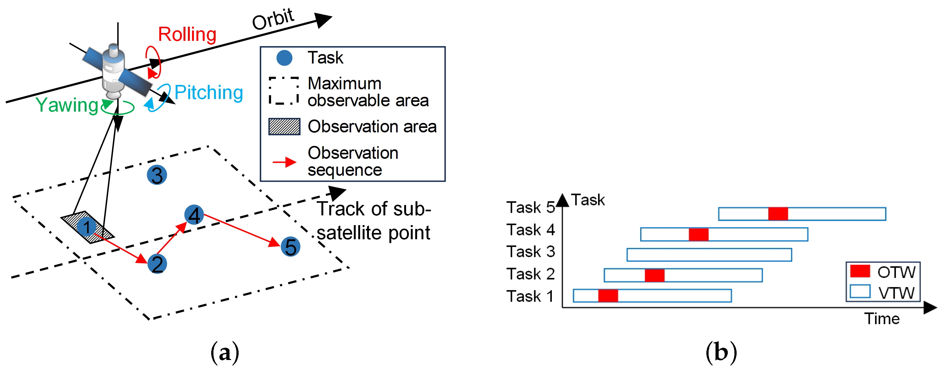
The multiple agile optical satellite scheduling problem (MAOSSP) aims to allocate observation tasks to AOSs and arrange their observation actions, satisfying complex constraints. As illustrated in Figure 1, an AOS executes observation tasks according to the scheduled order in the arranged time windows when flying over ground targets. The time window when the target is visible to the AOS is the visible time window (VTW), and the duration of the actual observation action is the observation time window (OTW). The agile attitude maneuverability of the AOSs expands the range of their observable areas and extends the length of the VTWs. However, MAOSSP is a complex scheduling problem whose complexity stems from three aspects. First, apart from conventional constraints, such as memory and energy limits, more complicated attitude maneuver constraints should be considered due to the agile characteristic of AOSs. For an AOS, the observation start time depends on its observation attitude, and the time interval between two adjacent observation actions must be sufficient enough for attitude adjustment, resulting in that the current observation action can influence the subsequent one [5]. Second, this problem has been proven as an NP-hard (non-deterministic polynomial hard) combination optimization problem [6], whose solution space grows dramatically with the rise of the problem scale. For one thing, the increase in the number of satellites provides more observation opportunities for each task but leads to a huge solution space with higher complexity. For another, the increase in the number of tasks turns this problem into an oversubscribed one [7,8], in which massive tasks are allocated to the limited satellite resources and can only be partially completed. Finally, the task allocation of satellites needs to consider not only the maximization of overall observation profit but also the load balance, which helps rationalize the daily management of satellites and prolong their lifetime [9].
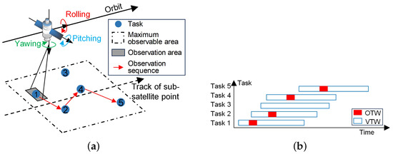
Figure 1.
Observation process of an AOS. (a) Determining the observation sequence of tasks. (b) Determining the observation time for tasks.
Existing methods for satellite scheduling can be generally classified into three categories: exact algorithms, heuristic algorithms, and deep reinforcement learning (DRL) algorithms. Exact algorithms can obtain the optimal solution by searching throughout the entire solution space but require a significant amount of computation time [10]. Thus, exact algorithms are only applicable to single-orbit or single-satellite scheduling scenarios. Heuristic algorithms can search for approximate solutions through population iteration. However, they can hardly tackle large-scale problems because the population iteration results in extensive constrain-check steps and enormous computation burden. In addition, premature convergence and local optimum are common problems for heuristic algorithms [11]. Differing from heuristic algorithms, DRL algorithms provide a non-iterative way to solve this problem, which constructs policy networks to generate solutions directly. DRL-based satellite scheduling methods can be divided into reinforcement learning (RL) approaches [12,13,14] and sequence-to-sequence (seq2seq) models [15,16]. The RL methods formulate the satellite scheduling process as a Markov decision process (MDP), which is an interaction process of agents and the environment, and a reward is given every time an agent chooses an action. In this process, the policy of the agent is continuously optimized through trial and error. The actions of agents only depend on the current environment state, making it hard to ensure the final action sequence can obtain a high-quality solution. Furthermore, the expansion of the problem scale leads to a rise in the decision dimensions, and it is challenging for MDP models to address the high-dimension problems. The seq2seq models use deep neural networks (DNN) based on the encoder-decoder structure [17] to construct a sequence in an auto-regressive way, which has superior abilities to handle long task sequences with high-dimension features. However, the current research can only achieve the “single-sequence-to-single-sequence” application and apply the seq2seq models to the single-satellite scheduling problems. Therefore, the seq2seq models need to be further explored to apply to the multi-satellite scheduling instances.
In this paper, we expand the current seq2seq models and propose a “single-sequence-to-multiple-sequence” model to solve the MAOSSP. In the proposed model, an unordered task sequence is input, and multiple task observation action sequences are output, each belonging to the corresponding satellite. The major contributions are summarized as follows.
- A mathematical model of the MAOSSP is established, whose optimization objective is to maximize the observation profit rate and realize the load balance. Meanwhile, a series of complex constraints are considered, such as the lighting condition, the flexible attitude maneuverability, the limitation of memory energy, and so on.
- A multi-pointer network is designed to construct high-quality scheduling solutions in an auto-regression manner, which provides a competitive DRL-based algorithm for this practical problem. Specifically, the network adopts multiple attention layers as the pointers to construct observation action sequences for multiple satellites. Furthermore, a local feature-enhancement strategy, a remaining time-based decoding sorting strategy, and a feasibility-based task selection strategy are proposed to improve the solving ability of the proposed network.
- Extensive experiments are conducted to verify the effectiveness of the proposed method. The experimental results validate that the proposed method has superior performance in solution quality, computational efficiency, and generalization ability in comparison with the state-of-the-art algorithms.
The remainder of this paper is organized as follows. Section 2 presents the recent research on the satellite scheduling problem. Section 3 gives a detailed description of the MAOSSP and builds the corresponding mathematical model. In Section 4, a multi-pointer network is proposed, and its architecture, components, and training algorithm are elaborated. Section 5 presents the experimental results, and Section 6 presents the conclusions of the study with a summary and directions for future work.
2. Related Work
In recent years, the Earth-observation satellite scheduling problem has received wide attention in the research literature, which can be roughly divided into exact methods, heuristic methods, and DRL methods.
When the problem scale is not too large, such as single-orbit or single-satellite scheduling scenarios, the exact algorithms can obtain the optimal solutions. Lemaître et al. [6] gave the general description of the agile satellite scheduling problem for the first time and proposed a dynamic programming algorithm. Chu et al. [18] presented a branch-and-bound algorithm with a look-ahead method and three pruning strategies to tackle the simplified agile satellite scheduling problem in a small-size instance. Peng et al. [5] considered the time-dependent profits and presented an adaptive-directional dynamic programming algorithm with decremental state space relaxation for the single-orbit scheduling of the single agile satellite. Qu et al. [19] developed a mixed integer linear programming model of the satellite scheduling problem and proposed an imitation learning framework for branch and bound to solve this model. The above studies summarily prove that exact algorithms can explore the whole search space and obtain the optimal solution, and they are applicable to single-orbit or small-scale satellite scheduling. However, as the problem scale expands, the computational cost of the exact algorithms tends to be unacceptable because of the NP-hard characteristic and the complex constraints.
Heuristic algorithms have been widely used to address the agile satellite scheduling problem owing to their outstanding search ability, such as the genetic algorithm (GA) [20,21], the particle swarm optimization (PSO) algorithm [22,23], the ant colony optimization (ACO) algorithm [24,25], the artificial bee colony (ABC) algorithm [26,27], and so on. Chatterjee and Chatterjee [28] established a mixed integer non-linear programming model to formulate the agile satellite scheduling problem with energy and memory constraints and proposed an elitist mixed coded genetic algorithm with a hill-climber mechanism to solve this problem. Zhou et al. [29] investigated the agile satellite scheduling problem of multiple observations with various durations and proposed an improved adaptive ant colony algorithm (IAACO) to solve this problem. This algorithm consisted of an adaptive task assignment layer with four operators and an observation time determination algorithm based on an improved ACO algorithm. Yang et al. [27] developed a hybrid discrete artificial bee colony algorithm (HDABC) for the imaging satellite mission planning problem. This algorithm improved the three search phases of the basic ABC algorithm to balance the exploitation exploration abilities of this algorithm and achieve population co-evolution. These heuristic algorithms exhibit satisfactory performance in solution quality through the iterative search of the population. However, heuristic algorithms suffer from the issues of long computation time and premature convergence. For one thing, each individual in the population needs complex constraint-checking steps, and the iterations of the population significantly increase the computational burden. For another, heuristic algorithms are prone to converge to the local optima because of the limitation of the search mechanisms.
In addition to these improvements for heuristic algorithms, some scholars have tried to utilize DRL approaches to improve population initialization and search operator selection. Wu et al. [30] presented a data-driven improved genetic algorithm to address the agile satellite scheduling problem, which adopted an artificial neural network to build the initial population, a frequent pattern mining approach to discover specific patterns from elite solutions, and three competition-based adaptive local adjustment strategies to maintain the diversity of the population. Song et al. [31] studied the electromagnetic detection satellite scheduling problem and proposed a genetic algorithm based on reinforcement learning (RLGA), which used Q-learning to guide the GA in choosing appropriate evolution operators. Based on this work, Song et al. [32] further investigated the multi-type satellite observation scheduling problem and developed a deep reinforcement learning-based genetic algorithm (DRL-GA). This algorithm used a dueling deep Q network to initialize the population, an individual update mechanism with an elite individual retention strategy to update the population, and a fast local search method with a DRL-assisted approach to construct neighborhood solutions. The applications of DRL have improved the exploration ability and computational efficiency of the heuristic algorithms, but the inherent issues of massive time consumption and premature convergence have not been thoroughly resolved.
Apart from combining the DRL methods with the heuristic algorithms, some attempts have been made to apply DRL algorithms to the agile satellite scheduling problem directly. Some research has formulated the agile satellite scheduling process as a Markov decision process and adopted RL algorithms to solve this problem. Specifically, Herrmann and Schaub [13] established an MDP model of the single agile satellite scheduling problem and adopted Monte Carlo tree search (MCTS) and supervised learning to train the policy networks of agents. The testing results showed that the performance of the trained policy networks approximated that of the MCTS policy, but its computational time was significantly reduced. Zhang et al. [33] presented a multi-agent MDP model of the multi-satellite collaborative scheduling problem and proposed a multi-agent reinforcement learning (MARL) method with the multi-agent proximal policy optimization (MAPPO) algorithm to solve this problem. Notably, the existing RL algorithms for satellite scheduling only adopt multi-layer fully connected neural networks as the policy networks, which can only handle the fixed-scale satellite scheduling problem. Once the number of tasks changes, the policy networks must be re-conducted and retrained. Therefore, these RL algorithms cannot be applicable to satellite scheduling problems with various scales. Inspired by the applications of seq2seq models in classical combination optimization fields, some scholars have developed excellent seq2seq models for the agile satellite scheduling problem. Zhao et al. [34] adopted the pointer network [35] to generate a permutation of executable tasks for the single-satellite scheduling problem. Wei et al. [17] studied the multi-objective agile satellite scheduling problem and constructed an encoder-decoder structure neural network to generate high-quality schedules. The constructed network consisted of a task encoder with a gated recurrent unit (GRU), a feature encoder with a convolution neural network (CNN), and a decoder with two attention layers. Long et al. [16] proposed a Transformer-based encoder-decoder network with temporal encoding for the Earth-observation scheduling problem with various scales. Due to the use of more advanced neural networks as policy networks, these seq2seq models can handle various satellite scheduling instances with different task scales. However, they can only generate one sequence for one satellite owing to the limitation of the network structures, so they cannot address the multi-satellite scheduling problems.
3. Problem Statement
The MAOSSP allocates tasks to satellites and arranges an observation action sequence for each satellite. A series of complex constraints must be considered in this problem, and its optimization objective is to maximize the observation profit rate and realize the load balance. In this section, we first make some simplifications and assumptions to standardize the MAOSSP and define some notions for the description of this problem. Then, a mathematical model is established to formulate this problem with complicated constraints and an optimization objective regarding the observation profit rate and the load balance.
3.1. Simplification and Assumption
The actual satellite scheduling process is complicated, and many complex practical factors make this problem difficult to describe [36,37], some of which do not need to be considered within the scope of the problem model [32]. For the convenience of problem modeling, some reasonable simplifications and assumptions are made based on the actual engineering background and the previous literature [16,32,37,38,39], which are listed as follows:
- Every task is a point target or a small strip, which can be covered through a single observation and cannot be decomposed or clustered.
- Every task can be executed at most once, and the execution process cannot be interrupted.
- Once a task is successfully scheduled, no uncertain factors will occur to affect its execution.
- The energy and memory of each satellite can recover to their maximum values at the beginning of each orbital period.
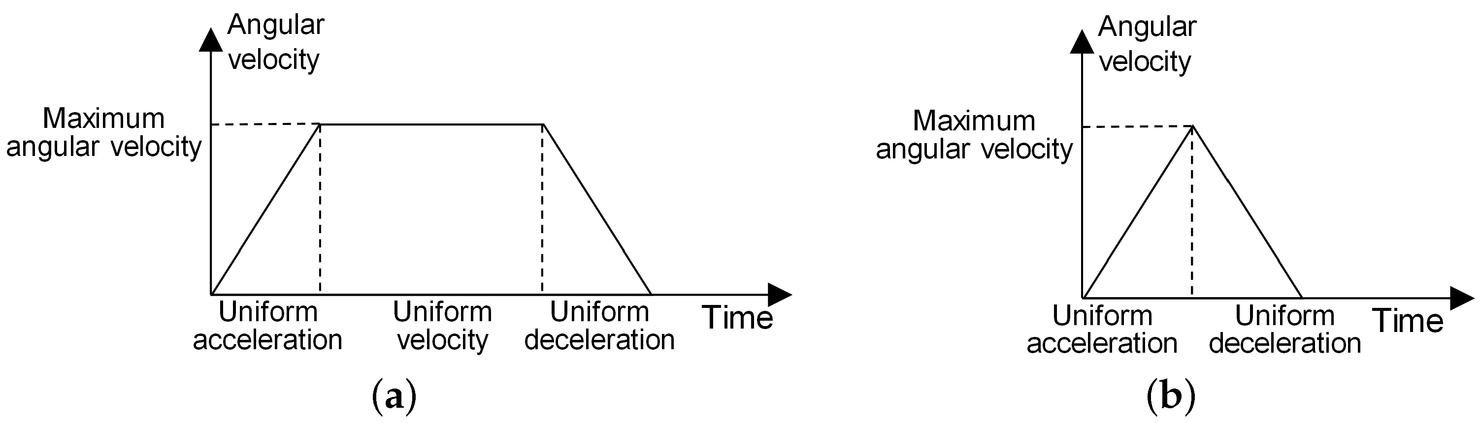
- For an AOS, the adjustment process of its pitch angle or roll angle is a “uniform acceleration-uniform velocity-uniform deceleration” process or a “uniform acceleration-uniform deceleration” process, as shown in Figure 2.
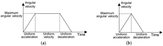 Figure 2. Angular adjustment process. (a) Uniform acceleration-uniform velocity-uniform deceleration. (b) Uniform acceleration-uniform deceleration.
3.2. Variable and Definition
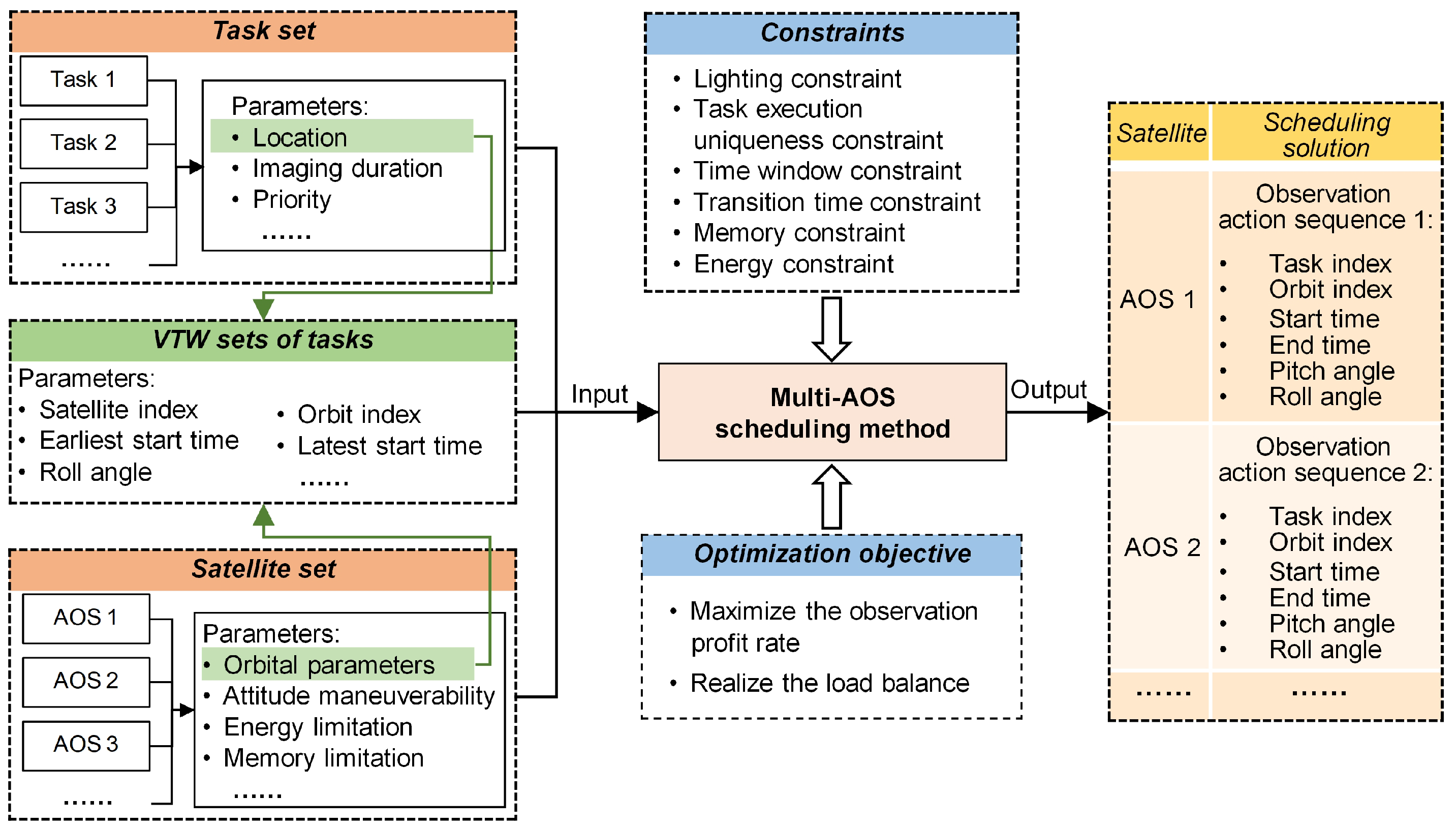
As shown in Figure 3, the inputs of the MAOSSP include a task set, a satellite set, and VTW sets of tasks, and the output scheduling solution consists of multiple observation action sequences. Before the formal solution, the VTW sets of all tasks are obtained according to the task location and the orbital parameters of satellites in the simulation system. In the solving process, the Multi-AOS scheduling method must fully consider a series of constraints, and its optimization objective is to maximize the observation profit rate and realize the load balance simultaneously.
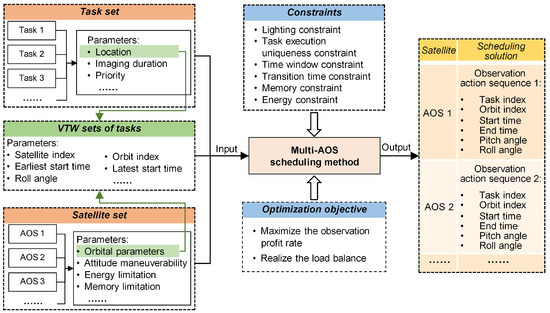
Figure 3.
Framework of MAOSSP.
To ease the description of the MAOSSP, the relevant variables are defined as follows:
- is the set of tasks, where is the number of tasks, and i is the task index. For the task i, the requirement information is denoted by , whose parameters are defined:
- −
- is the requested imaging duration;
- −
- is the priority, representing the observation profit.
- is the set of satellites, where is the number of satellites, j is the satellite index. For the satellite j, the following parameters are defined:
- −
- is the orbit set of the satellite j;
- −
- is the set of the periods that satisfy the lighting condition;
- −
- is the pitch angle range;
- −
- is the roll angle range;
- −
- a is the angular acceleration;
- −
- w is the maximum angular velocity;
- −
- is the angular adjustment time function, which is formulated as follows:where is the adjusted angle value on one axis; the derivation process of this function is presented in Appendix A;
- −
- M is the maximum memory for the storage of images;
- −
- is the memory consumption rate duration observation;
- −
- E is the maximum energy value used for observation and attitude adjustment;
- −
- is the energy consumption rate during observation;
- −
- is the energy consumption rate during angular adjustment.
- is the VTW set of the task i, and is the VTW set of the task i from satellite j, where is the number of VTWs, k is the VTW index. For the VTW , the following parameters are defined:
- −
- is the index of the orbit where this VTW is located;
- −
- is the earliest start time of this VTW;
- −
- is the latest start time of this VTW;
- −
- is the requested observation roll angle of this VTW.
- denotes the final multi-satellite scheduling solution, consisting of the observation action sequences of all satellites. is the observation action sequence of the satellite j. is the number of observation actions, which is also the number of tasks assigned to this satellite. is the lth observation action, whose parameters are defined as follows:
- −
- is the index of the task executed by this observation action;
- −
- is the index of the orbit where this observation action is executed;
- −
- is the OTW, where is the observation start time, and is the observation end time;
- −
- is the observation pitch angle;
- −
- is the observation roll angle.
- is the state vector of the satellite j after the observation action , where the observation end time is also the idle start time of this satellite, is the remaining memory, and is the remaining energy; is the initial state of the satellite j. and are formulated as follows:
- is a decision variable used to determine which VTW is selected for the task i, as formulated in Equation (4). Furthermore, the observation action () is a decision vector used to determine the observation action of the task i in the selected VTW.
3.3. Mathematical Model
According to the above variables, the observation profit rate is formulated in Equation (5), which is the ratio of the total profit of the executed tasks to the total profit of all tasks. The load balance is formulated in Equation (6) and denoted by a coefficient of variation of the number of tasks assigned to satellites, which is the ratio of the standard deviation to the average. The lower value of denotes that the scheduling solution performs better in load balance.
where is the average number of assigned tasks.
The optimization objective F is denoted by the difference between and , which is formulated as . The mathematical model of the MAOSSP is presented as follows:
Subject to:
Equation (7) denotes the optimization objective, and the higher value indicates that the scheduling solution is better. Equation (8) denotes the task execution uniqueness constraint that each task cannot be executed more than once. Equation (9) denotes the lighting constraint that each OTW must satisfy the lighting condition. Equation (10) denotes the time window constraint that every observation action must start in the corresponding VTW. Equation (11) denotes the transition time constraint that the time interval between two adjacent observation actions must be sufficient enough for angle adjustment. Equation (12) denotes the memory constraint that the remaining memory after an observation action must not be less than zero. Equation (13) denotes the energy constraint that the remaining energy after an observation action must not be less than zero.
4. Method
In this section, we propose a multi-pointer network for the MAOSSP. The architecture of the multi-pointer network, its components, and its training algorithm are elaborated in turn.
4.1. Architecture of the Multi-Pointer Network
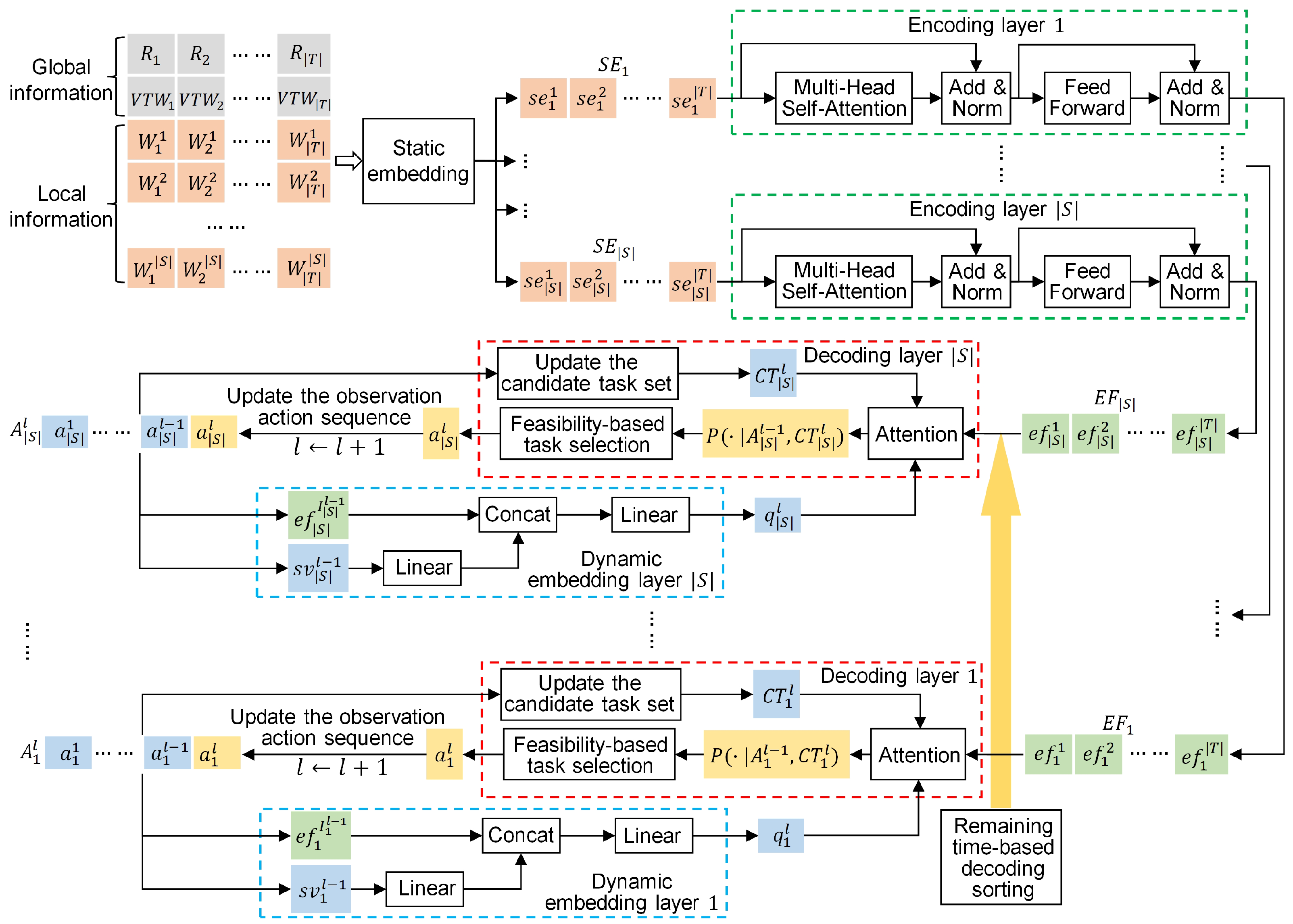
The existing seq2seq models [16,17,34] for satellite scheduling can only generate one observation action sequence for the single satellite. The core of these models is applying an attention model as a pointer to select an appropriate task for the satellite at every decoding step. To construct multiple observation action sequences for multi-satellite scheduling, we develop a multi-pointer network (MPN), as shown in Figure 4.
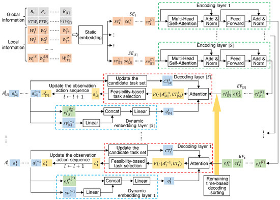
Figure 4.
The architecture of the multi-pointer network.
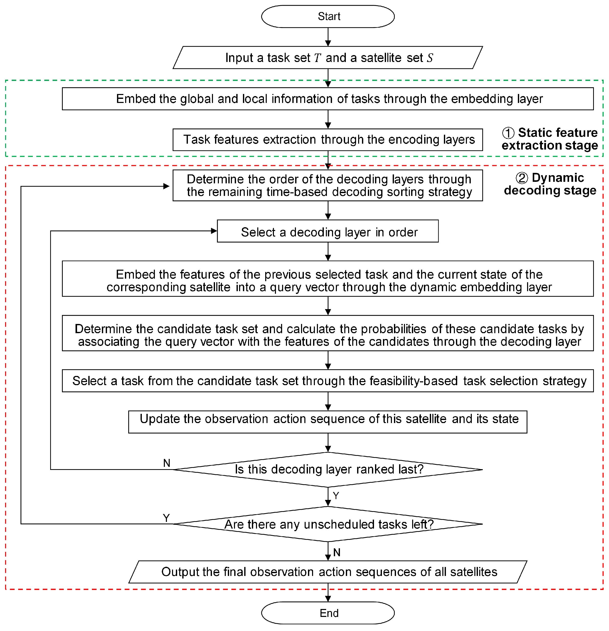
The most critical part of the MPN is that it adopts multiple attention layers as the multiple pointers, each of which is used to generate an observation action sequence for a different satellite. These attention layers belong to different decoding layers, and the number of decoding layers is equal to that of the satellites. In addition to the decoding layers, the important components of the MPN include a static embedding layer, multiple encoding layers, and multiple dynamic embedding layers. As shown in Figure 5, the workflow of this network model can be divided into two stages: a static feature extraction stage and a dynamic decoding stage, which is elaborated as follows:
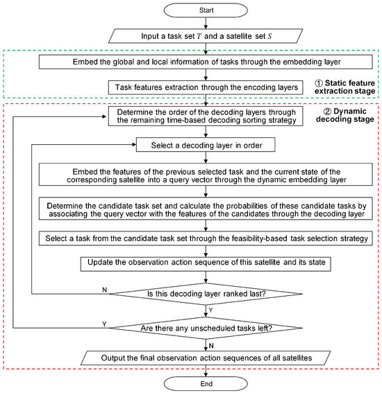
Figure 5.
The workflow of the multi-pointer network.
- Static feature extraction stage. In this stage, encoding layers with a static embedding layer are used to extract distinctive features from the input task information and provide them to the corresponding decoding layers. The input task information contains the requirements and VTW sets of the tasks. Considering that the VTWs of a task originate from different satellites, we classify the task information into global information and local information. For the task i, its global information contains its requirement information and the overall set of all its VTWs , and the VTW set that originates from the satellite j is the local information. A local feature-enhancement strategy is proposed to handle the input task information, which is described as follows:
- Local feature-enhancement strategy—First, the static embedding layer fuses the global information with the local information from different satellites and embeds the fusion results into a high-dimensional vector space. Then, the encoding layers further extract distinctive features from the embedding results with different local information. The local information embedding facilitates the local feature enhancement and can provide richer task features for decision-making.
- Dynamic decoding stage. In this stage, decoding layers, each equipped with a dynamic embedding layer, are used to construct the observation action sequences for the satellites. At every decoding step, the decoding process of these decoding layers is the same, and each decoding layer selects a task in turn. At the decoding step l, the dynamic embedding layer j is responsible for embedding the features of the previously selected task and the current state of the satellite j into a high-dimensional query vector. Next, the decoding layer j generates a set of candidate tasks and calculates the probabilities of candidate tasks by associating the query vector with the extracted task features provided to this decoding layer. The generation rule of the candidate task set is that the unscheduled task will be put into the candidate task set if it has at least one VTW in the remaining scheduling period of this satellite. Then, a candidate task is selected based on the probability distribution, and its observation action is determined through the earliest start time (EST) strategy, which sets the earliest feasible time as its observation start time. Finally, this observation action is placed at the end of the observation action sequence of the satellite j, and the state of this satellite is updated. The observation action sequence of the satellite j after l decoding steps is denoted as . Based on the above decoding process, a remaining time-based satellite sorting strategy and a feasibility-based task selection strategy are proposed to optimize the solution construction process, which is described as follows:
- Remaining time-based decoding sorting strategy—used to determine the decoding order of these decoding layers based on the remaining time of the corresponding satellites at the beginning of every decoding step. The remaining time of a satellite is the difference between the total scheduling time and its current idle start time. The shorter remaining time means fewer feasible tasks that can be allocated to this satellite, so the satellites with shorter remaining time should be ranked at the front in favor of the selection of more appropriate tasks. For this reason, this sorting strategy sorts these satellites in ascending order of their remaining time, and the order of these satellites is the decoding order of the corresponding decoding layers. If all the remaining unscheduled tasks do not have VTWs in the remaining period of a satellite, this satellite will be removed from the satellite set.
- Feasibility-based task selection strategy—used to select an appropriate task from the set of candidate tasks according to the probability distribution in every decoding layer. The proposed task selection strategy incorporates a feasibility-checking step based on the conventional greedy strategy. The task selection process with the proposed strategy is presented as follows. First, the candidate tasks are sorted in descending order of their probabilities. Second, these tasks are checked one by one to determine whether their observation actions can satisfy the constraints in Section 3.3. Once an observation action can satisfy these constraints, the corresponding will be selected, and this observation action will be added to the observation action sequence. If their observation actions do not meet these constraints, the candidate task set will be updated. This way ensures that each selected task is feasible.
4.2. Specific Structures of the Network Components
The multi-pointer network is composed of a static embedding layer, multiple encoding layers, multiple dynamic embedding layers, and multiple decoding layers, as shown in Figure 4. The number of these layers is related to the number of satellites. The specific structures of these components are elaborated as follows:
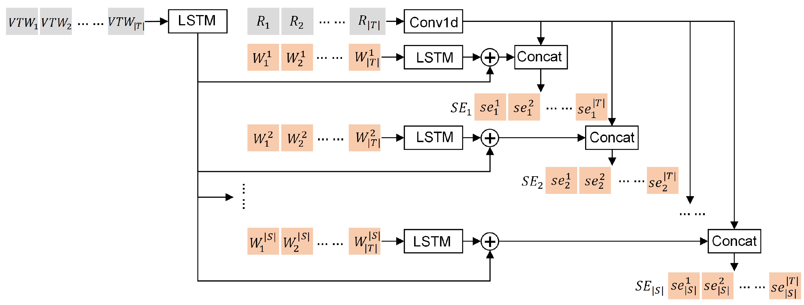
- Static embedding layer—used for the fusion and dimension conversion of the global and local task information. As shown in Figure 6, the static embedding layer consists of a one-dimensional convolution network () and LSTM networks (). is used to process the task requirements, is used to process the overall sets of all VTWs, and the left LSTMs are used to process the VTW sets from different satellites, respectively. For each task, the VTWs in its overall set of all VTWs are sorted in chronological order before being embedded. The final embedding results are denoted by a set , where is a high-dimensional embedding matrix provided to the encoding layer j. consists of embedding vectors, and is the embedding result of the task i for the encoding layer j. The generation process of is formulated as follows:where is a concatenation operator.
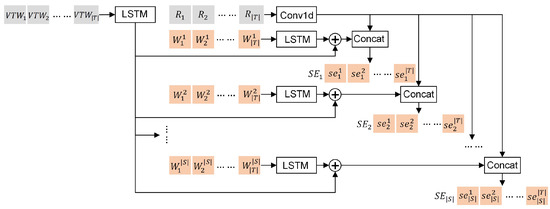 Figure 6. The structure of the embedding layer.
 - Encoding layers—extracting the distinctive features from the embedding results. These encoding layers have the same structure, each consisting of a multi-head self-attention layer (), a feed-forward layer (), and two residual connections. Each residual connection is composed of a skip-connection structure and a layer-normalization operator (). The encoding results are denoted by a set , where is a feature matrix provided to the decoding layer j. consists of feature vectors, and is the feature vector of the task i for the decoding layer j. The generation process of is formulated as follows:where is a process variable.
- Dynamic embedding layers—embedding the dynamic elements into a high-dimensional vector space and providing query vectors for the corresponding decoders at every decoding step. These dynamic embedding layers have the same structure, each consisting of two linear networks (). As for the dynamic embedding layer j, it embeds the feature vector of the previous selected task and the current state vector of the satellite j into a query vector at the decoding step l, which is formulated as follows:
- Decoding layers—selecting appropriate tasks for all satellites by associating the query vectors from the dynamic embedding layers with the extracted task features. These decoding layers have the same structure, and the main component of each one is an attention layer, whose learnable parameters are denoted by , , and . As for the decoding layer j, it obtains the probability distribution of the candidate tasks depending on the correlation between the query vector and the features of the candidate tasks. The set of the candidate tasks is denoted by , and a mask operator is used to mask the feature vectors of the tasks that are not in the candidate task set . The probability distribution is formulated in Equation (20). The probability of generating the final scheduling solution can be factorized according to the chain rule, as formulated in Equation (21).
4.3. Training Algorithm
The parameter of the MPN must be optimized by learning from abundant training samples, and the REINFORCE algorithm with baseline is adopted to train this network model, which is presented in Algorithm 1. The details of the training process are elaborated below.
| Algorithm 1: Training algorithm of the multi-pointer network |
|
First, given batches of training scenarios, some variables are defined to describe a batch of training scenarios: N denotes the batch size; denotes the task set in the nth scenario; denotes the output scheduling solution for the nth scenario; denotes the optimization objective value of , which is also the reward of this scheduling solution. Furthermore, is the number of training epochs, is the parameter of the MPN, and b is the baseline, the value of which is a constant.
Then, after a scheduling solution is generated, its reward can be calculated, and the probability can be obtained. After the scheduling of a batch of training instances is finished, the policy gradient of the MPN can be calculated, and the parameter of the MPN can be updated through the Adam optimizer, which is formulated as follows:
5. Computational Experiments
This section presents the computational experiments to demonstrate the effectiveness and the superiority of the MPN. First, the experimental settings are introduced, including the design of the datasets and the evaluation metrics. Second, a comparison experiment is carried out to verify the superiority of the MPN over some state-of-the-art algorithms for the MAOSSP. Third, an ablation experiment is constructed to verify the effectiveness of the proposed strategies in the MPN. These experiments are carried out on a laptop computer with Intel® CoreTM i7-7700HQ CPU@2.80 GHz and 40 GB RAM. The DRL framework embedded in Pytorch 1.5.1 in Python 3.8 is adopted in this study.
5.1. Experimental Settings
Due to the lack of a benchmark dataset, a large number of scenarios are designed based on the satellite scheduling scenario design method proposed by He et al. [4]. In these scenarios, the tasks are randomly distributed around the world. For each task, the requested imaging duration is a random integer between 5 and 10, and the priority is both random integers between 1 and 10. The orbital parameters of the satellites are available at https://celestrak.org/. The detailed scenario parameters are listed in Table 1. The scheduling time horizon is from 1 January 2023, 00:00:00, to 1 January 2023, 24:00:00.

Table 1.
Settings of scenario parameters.
Based on the above method, three training datasets and a testing dataset are created. Each training dataset contains 1920 training scenarios, in which the number of tasks is 1000, and the number of satellites is different. There are 10 satellites in the first training dataset, 15 satellites in the second training dataset, and 20 satellites in the third training dataset. The testing dataset contains several testing scenarios with various task and satellite scales. To distinguish the different testing scenarios, we used an “A-B-C” format to name them, where A is the number of satellites, B is the number of tasks, and C is the scenario number.
Three metrics are used to evaluate the performance of the testing results, including the final optimization objective F, the gap of the optimization objective , and the computation time. F represents the solution quality, and the higher F value indicates the better solution quality. The formula of F is given in Section 3.3. is used to enhance the assessment of the gap between the proposed MPN and comparison algorithms, which is formulated as follows:
where is the optimization objective value obtained by a comparison algorithm, and is the optimization objective value obtained by the MPN.
5.2. Training Performance
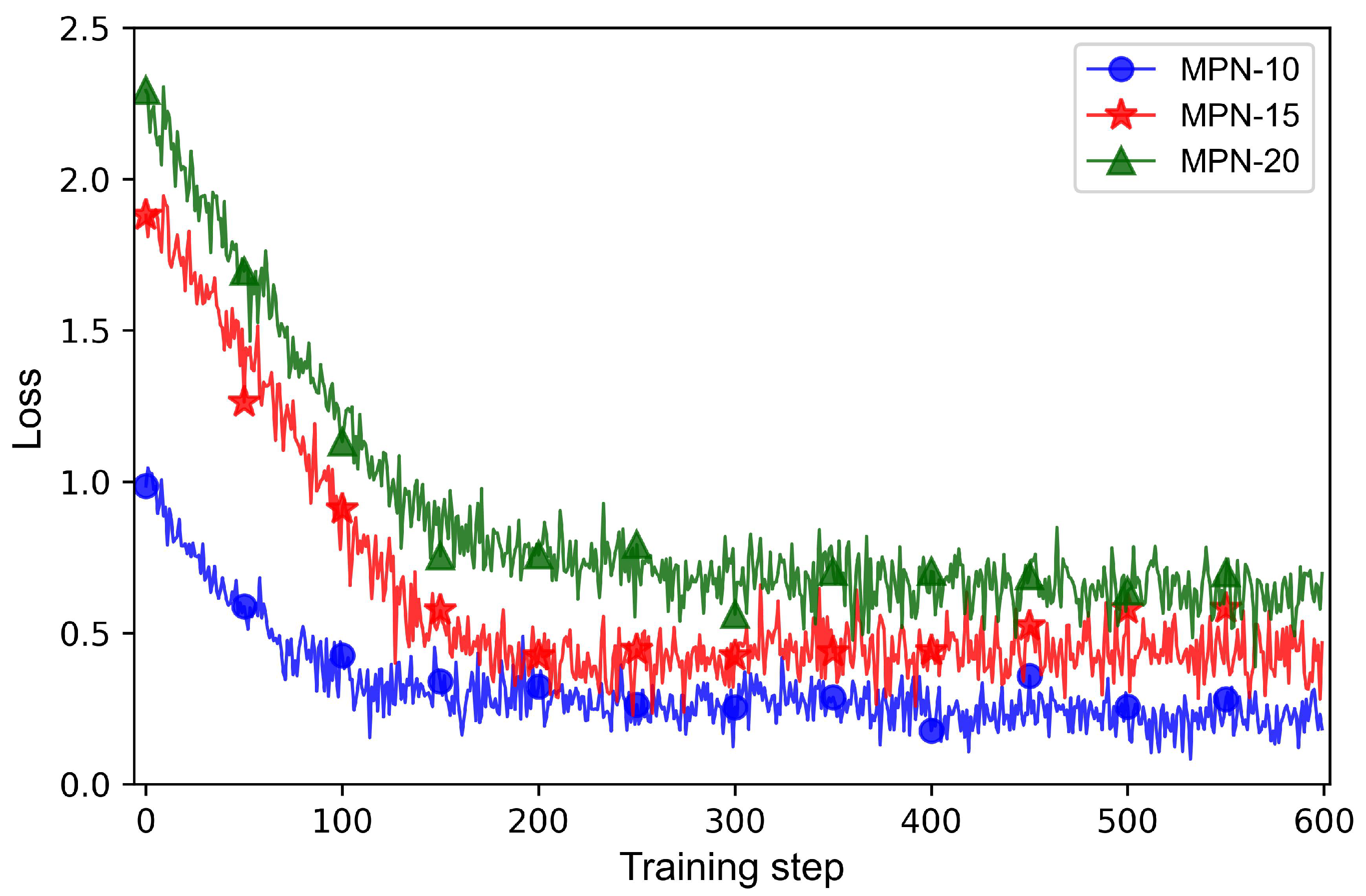
The MPNs for the scheduling scenarios with different satellite scales are trained on the three training datasets, respectively, and the trained networks are separately denoted by MPN-10, MPN-15, and MPN-20. The training parameters are listed in Table 2. Figure 7 depicts the loss curves of these three networks in the training process.
Table 2.
Settings of training parameters.
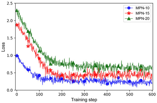
Figure 7.
Loss curves of MPN-10, MPN-15, and MPN-20.
As seen in Figure 7, the fluctuation of the three loss curves becomes smaller after 200 training steps, indicating that MPN-10, MPN-15, and MPN-20 can converge quickly. Furthermore, the three loss curves all converge to low levels, indicating that the training algorithm for the MPNs is effective.
5.3. Comparison with State-of-the-Art Algorithms
To verify the superiority of the trained MPNs, they are compared with four state-of-the-art multi-satellite scheduling algorithms, including IAACO [29], HDABC [27], RLGA [31], and MARL [33]. IAACO and HDABC are the improved heuristic algorithms, and RLGA is a combination of the reinforcement learning algorithm and the genetic algorithm. In these three algorithms, the size of population is set as 10, and the number of iterations is set as 100. MARL is a multi-agent reinforcement learning algorithm with MAPPO. The comparison experiment consists of two parts: the comparison in scenarios with 10 satellites and various task scales and the comparison in scenarios with more satellites and various task scales.
Table 3 and Table 4 present the testing results of the MPN-10 and the comparison algorithms in the scenarios with 10 satellites and various task scales, including the solution quality and the computation time. As shown in Table 3, the F values of MPN-10 are the highest among these algorithms, indicating that MPN-10 is significantly superior to the comparison algorithms in terms of the solution quality. Furthermore, the values of IAACO and HDABC are higher than those of RLGA and MARL, indicating that the heuristic algorithms are inferior to the deep reinforcement learning algorithms in terms of the solving ability. Moreover, the values of the comparison algorithms tend to be higher with the increase in the number of tasks, indicating the more significant superiority of MPN-10 in the scenarios with lager task scales. As listed in Table 4, MPN-10 takes the least computation among these algorithms, indicating that MPN-10 is superior to the comparison algorithms in terms of computation efficiency. In particular, the computation time of MPN-10 is much lower than that of IAACO and HDABC owing to the fact that the MPN constructs the solutions in an end-to-end manner, which does not need the iterations of the population. From a comprehensive perspective of solution quality and computation time, the proposed MPN exhibits excellent performance in solving ability and computation efficiency.
Table 3.
Comparison of the solution quality in the scenarios with 10 satellites and various task scales.
Table 4.
Comparison of the computation time (in seconds) in the scenarios with 10 satellites and various task scales.
Table 5 and Table 6 present the testing results of the MPN-15 and MPN-20 and the comparison algorithms in the scenarios with more satellites and various task scales. As illustrated in Table 5, MPN-15 achieves the best F values in the15-satellite scenarios, and MPN-20 obtains the best F values in the 20-satellite scenarios, demonstrating that the proposed MPN has a superior generalization ability over the comparison algorithms to apply to the various-scale scenarios. In particular, the MPN performs much better in the scenarios with more satellites, meaning that the MPN is applicable to large-scale satellite scheduling scenarios. As illustrated in Table 6, MPN-15 takes the least computation time in the 15-satellite scenarios, and MPN-20 takes the least computation time in the 20-satellite scenarios, demonstrating that the proposed MPN is superior to the comparison algorithms in terms of the computation efficiency.
Table 5.
Comparison of the solution quality in the scenarios with more satellites and various task scales.
Table 6.
Comparison of the computation time (in seconds) in the scenarios with more satellites and various task scales.
Overall, the solving ability, computation efficiency, and generalization of the proposed MPN have been verified through the above comparison experiments on extensive testing scenarios. First, the performance of the MPN is better than that of the comparison algorithms in terms of solution quality and computation efficiency. Second, the gaps between the comparison algorithms and the MPN rise gradually with the increase in the task scale, demonstrating the superior solving ability of the MPN to tackle scheduling scenarios with large-scale tasks. Third, the overall performance of the MPN is still better than that of the comparison algorithms in the scenarios with more satellites, demonstrating the superior generalization ability of the MPN to apply to various-scale scheduling scenarios.
5.4. Ablation Study
In the proposed MPN, a local feature-enhancement strategy is used to extract richer task features in the static feature extraction stage, and a remaining time-based decoding sorting strategy and a feasibility-based task selection strategy are used to improve the solution construction process in the dynamic decoding stage. To verify the effectiveness of these three strategies, we compare the performance of the MPN to that of the MPNs without one of these strategies. MPN-10 is the MPN with all these three strategies, and the comparison MPNs lack a strategy but are equipped with the other two strategies.
Table 7 lists the testing results of these MPNs with different strategies in the 10-satellite scenarios with different task scales. In terms of the solution quality, MPN-10 performs the best among these MPNs, demonstrating that the proposed strategies are beneficial for improving the solution quality. The value of the MPN without the remaining time-based decoding sorting strategy is higher than that of the other two MPNs in all testing scenarios, indicating that the remaining time-based decoding sorting strategy plays a more important role in the improvement of the solution quality compared to the local feature-enhancement strategy and the feasibility-based task selection strategy. In most testing scenarios, MPN-10 takes the most computation time, and the MPN without the local feature-enhancement strategy takes the least computation time, indicating that these strategies need a little more computation time and that the local feature-enhancement strategy needs the most among them. From a comprehensive perspective of solution quality and computation time, these three strategies result in a slight increase in the computation burden but significantly improve the solution quality.
Table 7.
Comparison results of the MPNs with different strategies.
Table 8 lists the observation profit rate and the load balance obtained by the MPNs with different strategies in the 10-satellite scenarios with various task scales. and are described in Section 3.3. In terms of the load balance , MPN-10 performs the best in most testing scenarios whose task scales do not exceed 1000, while MPN-10 achieves the highest values when the number of tasks is more than 1000. However, MPN-10 is superior to the other MPNs in all testing scenarios in terms of the observation profit rate , indicating that these three strategies significantly improve the solution quality, especially in the aspect of the improvement of the observation profit rate. Furthermore, the MPN with the feasibility-based task selection strategy obtains the lowest values in all these testing scenarios, indicating that the improvement of the solution quality from the feasibility-based task selection strategy lies in the enhancement of the observation profit rate.
Table 8.
and obtained by the MPNs with different strategies.
Overall, the effectiveness of the proposed three strategies has been verified through the above ablation experiment. First, the MPN with all these strategies shows better performance in the solution quality than the other MPNs, demonstrating that these strategies effectively enhance the solving ability of the MPN. Second, these strategies significantly improve the observation profit rate obtained by the MPN, resulting in the improvement of the solution quality. Third, the feasibility-based task selection strategy plays a more significant role in improving the solution quality than the other two strategies.
6. Conclusions
In this paper, a multi-pointer network is proposed to solve the multi-agile optical satellite scheduling problem considering the observation profit rate and the load balance. This network is a “single-sequence-to-multiple-sequence” model, which adopts multiple attention layers as the pointers to construct observation action sequences for multiple satellites. Three strategies are proposed to improve the solving ability of the proposed network: first, a local feature-enhancement strategy is adopted to fuse the global task information with the local task information, beneficial for providing more distinctive and richer task features for decision-making; second, a remaining time-based decoding sorting strategy is applied to arrange the sort of the decoding layers based on the remaining time of the corresponding satellites, facilitating the selection of appropriate tasks for satellites; third, a feasibility-based task selection strategy is used to select executable tasks for satellites, avoiding the generation of the infeasible solution. Based on these strategies, the proposed network shows excellent performance in solution quality, computation efficiency, and generalization ability compared to four state-of-the-art algorithms. The ablation experiment fully demonstrates the effectiveness of these three strategies in the improvement of the solution quality.
For future work, we will investigate the uncertain scheduling problem of multiple agile optical satellites and consider the uncertain factors in this problem, such as the effect of cloud cover and the dynamic arrival of emergency tasks. The effective solution to this problem usually requires a real-time or near real-time scheduling method to adapt to the dynamic changes in uncertain factors. Therefore, we will further explore the proposed network model to extend it to this uncertain multi-satellite scheduling problem.
Author Contributions
Conceptualization, Z.L. and W.X.; methodology, Z.L. and W.X.; software, Z.L. and C.H.; validation, Z.L.; formal analysis, Z.L.; investigation, Z.L. and C.H.; resources, C.H. and K.Z.; data curation, K.Z.; writing—original draft preparation, Z.L.; writing—review and editing, Z.L. and W.X.; visualization, Z.L. and C.H.; supervision, W.X.; project administration, W.X.; funding acquisition, W.X. All authors have read and agreed to the published version of the manuscript.
Funding
This research was funded by Aerospace Discipline Education New Engineering Project, grant number 145AXL250004000X.
Data Availability Statement
Data are contained within the article.
Conflicts of Interest
The authors declare no conflicts of interest.
Abbreviations
The following abbreviations are used in this manuscript:
| AOS | Agile optical satellite scheduling |
| MAOSSP | Multi-agile optical satellite scheduling problem |
| VTW | Visible time window |
| OTW | Observation time window |
| NP | Non-deterministic polynomial |
| DRL | Deep reinforcement learning |
| RL | Reinforcement learning |
| Seq2Seq | Sequence-to-sequence |
| MDP | Markov decision process |
| DNN | Deep neural network |
| GA | Genetic algorithm |
| PSO | Particle swarm optimization |
| ACO | Ant colony optimization |
| ABC | Artificial bee colony |
| IAACO | Improved adaptive ant colony algorithm |
| HDABC | Hybrid discrete artificial bee colony algorithm |
| RLGA | Genetic algorithm based on reinforcement learning |
| DRL-GA | Deep reinforcement learning-based genetic algorithm |
| MCTS | Monte Carlo tree search |
| MARL | Multi-agent reinforcement learning |
| MAPPO | Multi-agent proximal policy optimization |
| GRU | Gated recurrent unit |
| CNN | Convolution neural network |
| MPN | Multi-pointer network |
| EST | Earliest start time |
| LSTM | Long short-term memory |
| MHSA | Multi-head self-attention |
| FF | Feed-forward |
| LN | layer-normalization |
Appendix A
The derivation process of the angular adjustment time function is described as follows.
First, for an AOS, the adjustment process of its pitch angle or roll angle is regarded as a “uniform acceleration-uniform velocity-uniform deceleration” process or a “uniform acceleration-uniform deceleration” process, which is shown in Figure 2. Based on this assumption, some variables are redefined to describe this process. is the adjustment value of an angular; w is the maximum angular velocity; a is the angular acceleration value; is the adjustment time, and . The time required for the angular velocity to accelerate from 0 to its maximum value w is denoted by , which is formulated as follows:
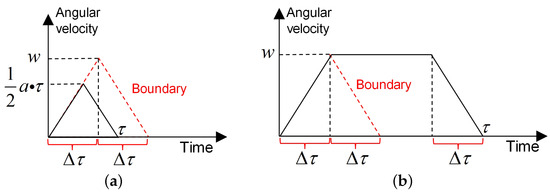
Figure A1.
Angular adjustment process. (a) Uniform acceleration-uniform deceleration. (b) Uniform acceleration-uniform velocity-uniform deceleration.
Figure A1.
Angular adjustment process. (a) Uniform acceleration-uniform deceleration. (b) Uniform acceleration-uniform velocity-uniform deceleration.
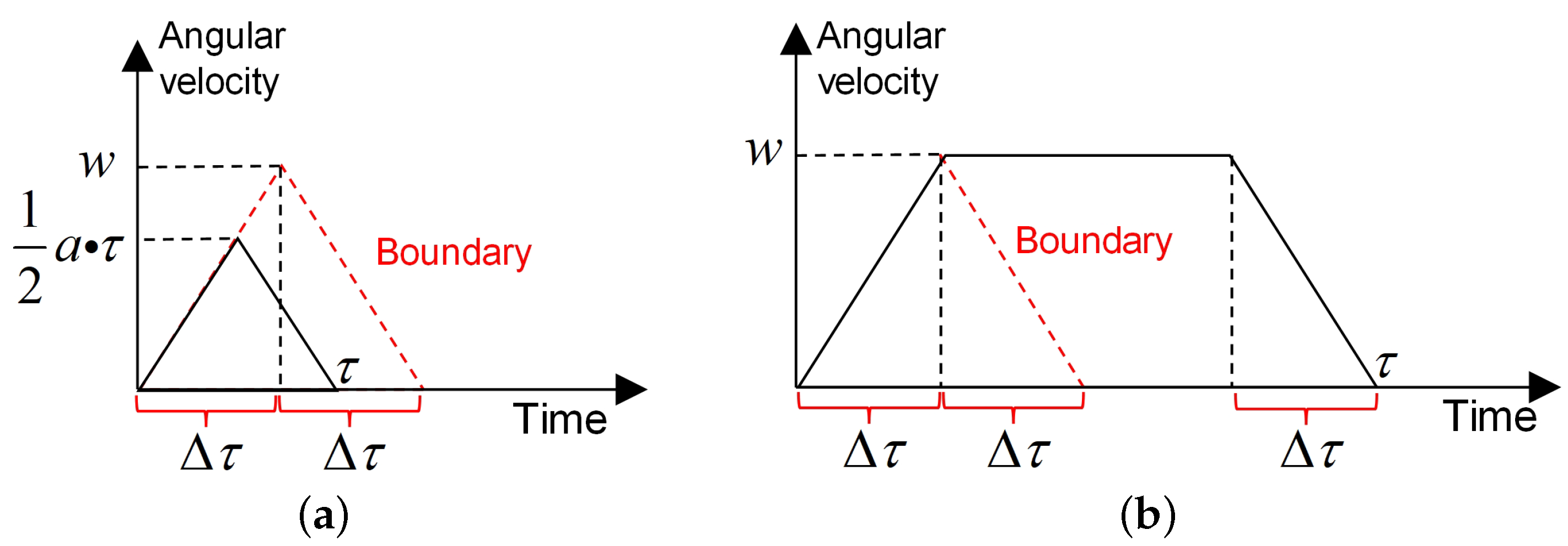
Second, when the adjustment value of the angular is small, this angular adjustment process is a “uniform acceleration-uniform deceleration” process, as shown in Figure A1a; and it is a “uniform acceleration-uniform velocity-uniform deceleration” process when the adjustment value of the angular exceeds a certain value, as shown in Figure A1b. The boundary value of the angular is denoted by , and it can be formulated as follows:
Third, when , the area of the triangle with the black line in Figure A1a is equal to , which is formulated as follows:
Then, the required adjustment time is formulated as follows:
Fourth, when , the area of the trapezoid with the black line in Figure A1b is equal to , which is formulated as follows:
Then, the required adjustment time is formulated as follows:
The above is the derivation process of the angular adjustment time function .
References
- Onojeghuo, A.O.; Blackburn, G.A.; Huang, J.; Kindred, D.; Huang, W. Applications of satellite ‘hyper-sensing’in Chinese agriculture: Challenges and opportunities. Int. J. Appl. Earth Obs. Geoinf. 2018, 64, 62–86. [Google Scholar]
- Hede, A.N.H.; Koike, K.; Kashiwaya, K.; Sakurai, S.; Yamada, R.; Singer, D.A. How can satellite imagery be used for mineral exploration in thick vegetation areas? Geochem. Geophys. Geosyst. 2017, 18, 584–596. [Google Scholar] [CrossRef]
- Han, C.; Xiong, W.; Xiong, M.; Liu, Z. Support vector regression-based operational effectiveness evaluation approach to reconnaissance satellite system. J. Syst. Eng. Electron. 2023, 34, 1626–1644. [Google Scholar] [CrossRef]
- He, Y.; Xing, L.; Chen, Y.; Pedrycz, W.; Wang, L.; Wu, G. A generic Markov decision process model and reinforcement learning method for scheduling agile earth observation satellites. IEEE Trans. Syst. Man Cybern. Syst. 2020, 52, 1463–1474. [Google Scholar] [CrossRef]
- Peng, G.; Song, G.; He, Y.; Yu, J.; Xiang, S.; Xing, L.; Vansteenwegen, P. Solving the agile earth observation satellite scheduling problem with time-dependent transition times. IEEE Trans. Syst. Man Cybern. Syst. 2020, 52, 1614–1625. [Google Scholar] [CrossRef]
- Lemaître, M.; Verfaillie, G.; Jouhaud, F.; Lachiver, J.M.; Bataille, N. Selecting and scheduling observations of agile satellites. Aerosp. Sci. Technol. 2002, 6, 367–381. [Google Scholar] [CrossRef]
- Wang, X.; Han, C.; Zhang, R.; Gu, Y. Scheduling multiple agile earth observation satellites for oversubscribed targets using complex networks theory. IEEE Access 2019, 7, 110605–110615. [Google Scholar] [CrossRef]
- Xiong, M.; Xiong, W.; Liu, Z. A co-evolutionary algorithm with elite archive strategy for generating diverse high-quality satellite range schedules. Complex Intell. Syst. 2023, 9, 5157–5172. [Google Scholar] [CrossRef]
- Wei, L.; Xing, L.; Wan, Q.; Song, Y.; Chen, Y. A multi-objective memetic approach for time-dependent agile earth observation satellite scheduling problem. Comput. Ind. Eng. 2021, 159, 107530. [Google Scholar] [CrossRef]
- Chu, X.; Chen, Y.; Xing, L. A branch and bound algorithm for agile earth observation satellite scheduling. Discret. Dyn. Nat. Soc. 2017, 2017, 7345941. [Google Scholar] [CrossRef]
- Zheng, Z.; Guo, J.; Gill, E. Swarm satellite mission scheduling & planning using hybrid dynamic mutation genetic algorithm. Acta Astronaut. 2017, 137, 243–253. [Google Scholar]
- Ren, L.; Ning, X.; Wang, Z. A competitive Markov decision process model and a recursive reinforcement-learning algorithm for fairness scheduling of agile satellites. Comput. Ind. Eng. 2022, 169, 108242. [Google Scholar] [CrossRef]
- Herrmann, A.; Schaub, H. Reinforcement learning for the agile earth-observing satellite scheduling problem. IEEE Trans. Aerosp. Electron. Syst. 2023, 59, 5235–5247. [Google Scholar] [CrossRef]
- Li, G.; Li, X.; Li, J.; Chen, J.; Shen, X. PTMB: An online satellite task scheduling framework based on pre-trained Markov decision process for multi-task scenario. Knowl.-Based Syst. 2024, 284, 111339. [Google Scholar] [CrossRef]
- Wang, X.; Wu, J.; Shi, Z.; Zhao, F.; Jin, Z. Deep reinforcement learning-based autonomous mission planning method for high and low orbit multiple agile Earth observing satellites. Adv. Space Res. 2022, 70, 3478–3493. [Google Scholar] [CrossRef]
- Long, Y.; Shan, C.; Shang, W.; Li, J.; Wang, Y. Deep Reinforcement Learning-Based Approach With Varying-Scale Generalization for the Earth Observation Satellite Scheduling Problem Considering Resource Consumptions and Supplements. IEEE Trans. Aerosp. Electron. Syst. 2024, 60, 2572–2585. [Google Scholar] [CrossRef]
- Wei, L.; Chen, Y.; Chen, M.; Chen, Y. Deep reinforcement learning and parameter transfer based approach for the multi-objective agile earth observation satellite scheduling problem. Appl. Soft Comput. 2021, 110, 107607. [Google Scholar] [CrossRef]
- Chu, X.; Chen, Y.; Tan, Y. An anytime branch and bound algorithm for agile earth observation satellite onboard scheduling. Adv. Space Res. 2017, 60, 2077–2090. [Google Scholar] [CrossRef]
- Qu, Q.; Liu, K.; Li, X.; Zhou, Y.; Lü, J. Satellite observation and data-transmission scheduling using imitation learning based on mixed integer linear programming. IEEE Trans. Aerosp. Electron. Syst. 2022, 59, 1989–2001. [Google Scholar] [CrossRef]
- Hosseinabadi, S.; Ranjbar, M.; Ramyar, S.; Amel-Monirian, M. Scheduling a constellation of agile Earth observation satellites with preemption. J. Qual. Eng. Prod. Optim. 2017, 2, 47–64. [Google Scholar]
- Mao, L.; Qing, D.; Liu, R.; Kong, X. CPM-GA for Multi-satellite and Multi-task Simulation Scheduling. J. Syst. Simul. 2021, 33, 205–214. [Google Scholar]
- Yan, B.; Wang, Y.; Xia, W.; Hu, X.; Ma, H.; Jin, P. An improved method for satellite emergency mission scheduling scheme group decision-making incorporating PSO and MULTIMOORA. J. Intell. Fuzzy Syst. 2022, 42, 3837–3853. [Google Scholar] [CrossRef]
- Wu, X.; Yang, Y.; Sun, Y.; Xie, Y.; Song, X.; Huang, B. Dynamic regional splitting planning of remote sensing satellite swarm using parallel genetic PSO algorithm. Acta Astronaut. 2023, 204, 531–551. [Google Scholar] [CrossRef]
- Cui, K.; Xiang, J.; Zhang, Y. Mission planning optimization of video satellite for ground multi-object staring imaging. Adv. Space Res. 2018, 61, 1476–1489. [Google Scholar] [CrossRef]
- He, L.; Liu, X.L.; Chen, Y.W.; Xing, L.N.; Liu, K. Hierarchical scheduling for real-time agile satellite task scheduling in a dynamic environment. Adv. Space Res. 2019, 63, 897–912. [Google Scholar] [CrossRef]
- Luo, K. A hybrid binary artificial bee colony algorithm for the satellite photograph scheduling problem. Eng. Optim. 2020, 52, 1421–1440. [Google Scholar] [CrossRef]
- Yang, Y.; Liu, D. A hybrid discrete artificial bee colony algorithm for imaging satellite mission planning. IEEE Access 2023, 11, 40006–40017. [Google Scholar] [CrossRef]
- Chatterjee, A.; Tharmarasa, R. Reward factor-based multiple agile satellites scheduling with energy and memory constraints. IEEE Trans. Aerosp. Electron. Syst. 2022, 58, 3090–3103. [Google Scholar] [CrossRef]
- Zhou, Z.; Chen, E.; Wu, F.; Chang, Z.; Xing, L. Multi-satellite scheduling problem with marginal decreasing imaging duration: An improved adaptive ant colony algorithm. Comput. Ind. Eng. 2023, 176, 108890. [Google Scholar] [CrossRef]
- Wu, J.; Song, B.; Zhang, G.; Ou, J.; Chen, Y.; Yao, F.; He, L.; Xing, L. A data-driven improved genetic algorithm for agile earth observation satellite scheduling with time-dependent transition time. Comput. Ind. Eng. 2022, 174, 108823. [Google Scholar] [CrossRef]
- Song, Y.; Wei, L.; Yang, Q.; Wu, J.; Xing, L.; Chen, Y. RL-GA: A reinforcement learning-based genetic algorithm for electromagnetic detection satellite scheduling problem. Swarm Evol. Comput. 2023, 77, 101236. [Google Scholar] [CrossRef]
- Song, Y.; Ou, J.; Pedrycz, W.; Suganthan, P.N.; Wang, X.; Xing, L.; Zhang, Y. Generalized model and deep reinforcement learning-based evolutionary method for multitype satellite observation scheduling. IEEE Trans. Syst. Man Cybern. Syst. 2024, 54, 2576–2589. [Google Scholar] [CrossRef]
- Zhang, G.; Li, X.; Hu, G.; Li, Y.; Wang, X.; Zhang, Z. MARL-Based Multi-Satellite Intelligent Task Planning Method. IEEE Access 2023, 11, 135517–135528. [Google Scholar] [CrossRef]
- Zhao, X.; Wang, Z.; Zheng, G. Two-phase neural combinatorial optimization with reinforcement learning for agile satellite scheduling. J. Aerosp. Inf. Syst. 2020, 17, 346–357. [Google Scholar] [CrossRef]
- Vinyals, O.; Fortunato, M.; Jaitly, N. Pointer networks. Adv. Neural Inf. Process. Syst. 2015, 28, 2692–2700. [Google Scholar]
- Ren, L.; Ning, X.; Li, J. Hierarchical reinforcement-learning for real-time scheduling of agile satellites. IEEE Access 2020, 8, 220523–220532. [Google Scholar] [CrossRef]
- Wang, X.; Wu, G.; Xing, L.; Pedrycz, W. Agile earth observation satellite scheduling over 20 years: Formulations, methods, and future directions. IEEE Syst. J. 2020, 15, 3881–3892. [Google Scholar] [CrossRef]
- He, L.; de Weerdt, M.; Yorke-Smith, N. Time/sequence-dependent scheduling: The design and evaluation of a general purpose tabu-based adaptive large neighbourhood search algorithm. J. Intell. Manuf. 2020, 31, 1051–1078. [Google Scholar] [CrossRef]
- Zhang, J.; Xing, L. An improved genetic algorithm for the integrated satellite imaging and data transmission scheduling problem. Comput. Oper. Res. 2022, 139, 105626. [Google Scholar] [CrossRef]
Disclaimer/Publisher’s Note: The statements, opinions and data contained in all publications are solely those of the individual author(s) and contributor(s) and not of MDPI and/or the editor(s). MDPI and/or the editor(s) disclaim responsibility for any injury to people or property resulting from any ideas, methods, instructions or products referred to in the content. |
© 2024 by the authors. Licensee MDPI, Basel, Switzerland. This article is an open access article distributed under the terms and conditions of the Creative Commons Attribution (CC BY) license (https://creativecommons.org/licenses/by/4.0/).