Clustering and Cooperative Guidance of Multiple Decoys for Defending a Naval Platform Against Salvo Threats

Abstract

The threat to naval platforms from missile systems is increasing due to recent advancements in radar seeker technology, which have significantly enhanced the accuracy and effectiveness of missile targeting. In scenarios where a naval platform with limited maneuverability faces salvo attacks, the importance of an effective defense strategy becomes crucial to ensuring the protection of the platform. In this study, we present a multi-agent reinforcement learning-based decoy deployment approach that employs six decoys to increase the survival likelihood of a naval platform against salvo missile strikes. Our approach entails separating the decoys into two clusters, each consisting of three decoys. Subsequently, every cluster is allocated to a related missile threat. This is accomplished by training the decoys with the multi-agent deep reinforcement learning algorithm. To compare the proposed approach across different algorithms, we use two distinct algorithms to train the decoys; multi-agent deep deterministic policy gradient (MADDPG) and multi-agent twin-delayed deep deterministic policy gradient (MATD3). Following training, the decoys learn to form groups and establish effective formation configurations within each group to ensure optimal coordination. We assess the proposed decoy deployment strategy using parameters including decoy deployment angle and maximum decoy speed. Our findings indicate that decoys positioned on the same side outperform those positioned on different sides relative to the target platform. In general, MATD3 performs slightly better than MADDPG. Decoys trained with MATD3 succeed in more successful formation configurations than those trained with the MADDPG method, which accounts for this enhancement.

1. Introduction

Originating in the 1980s, digital radio frequency memory (DRFM) technology has undergone significant advancements, transitioning from basic mono-bit devices to sophisticated wideband, high dynamics range systems. The DRFM is a crucial component in modern radar jamming systems. It is capable of creating false targets possessing all the characteristics of the actual target. The concept of DRFM technology is outlined in [1], explaining its underlying principles and discussing its use in ECM systems. Moreover, the study specifically addresses the vital variables that impact the performance of the DRFM systems and thoroughly examines a variety of architectures. A new method in [2] is proposed to improve electronic countermeasures capabilities against pulse-type radar systems by conducting the setup DRFM system. The authors focused on developing a DRFM system designed to sample and quantize incoming pulse-type radar signals. Reference [3] highlighted a groundbreaking RF system architecture for small flying drones, containing radar transmission, reception, and jamming functionalities on a single FPGA-based platform. The research thoroughly investigated the key determinants that affect the effectiveness of electronic attacks on coherent radars, providing useful insights on how to develop functional EAs. The relative motion of the DRFM jammer to the designated radar raises some challenges in the stand-in-jamming (SIJ) scenario. Reference [4] specifically addressed the difficulties posed by the relative motion and provided tactics to enhance jamming effectiveness within dynamic environments. The approach suggested is verified through simulations generated by MATLAB (R2020a, MathWorks) program and Verilog implementation. Reference [5] examined the importance of employing numerous UAVs in electronic attack operations. The authors outlined the technical difficulties and possible remedies for effectively leveraging multiple UAVs in EW scenarios. Furthermore, the research emphasizes the need for cooperative control of UAVs and suggests approaches aimed at enhancing efficiency, and endurance, and minimizing exposure to threats. In [6], the authors tackled the issue of manipulating RADAR systems through the use of cooperative UAVs to generate a “phantom” aircraft to confound the RADAR systems. The focus of the study revolved around developing a cooperative control system, facilitating UAVs for successfully misleading RADAR systems. Reference [7] addressed the challenge of organizing multiple UAVs for cooperative decoy jamming against an ISAR radar system, with a particular emphasis on distributed and cooperative decision-making. The utilization of a decentralized model predictive control algorithm enables multi-UAV systems for the self-organization and achievement of collective radar signatures within electronic warfare environments. Reference [8] focused on enhancing the survivability of ships against enemy torpedoes through the utilization of single and multiple decoy deployments. The authors assessed various deployment tactics, such as same-side deployment and zig-zag deployment, and demonstrated that zig-zag deployment yielded superior effectiveness compared to same-side deployment. Reference [9] examined missile avoidance trajectories in conjunction with off-board countermeasures, particularly flares and air-launched decoys. The authors developed an analytical expression for miss distance and conducted simulation scenarios to evaluate the results. The results suggest that the simultaneous utilization of countermeasures proves successful in avoiding missile attacks in aircraft scenarios. Reference [10] focused on the difficulty of path planning for joint-force electronic attacks carried out by unmanned aerial vehicles (UAVs) operating in hostile environments. The paper examined numerous cooperation methods, including the use of jamming resources against tracking radars, and assessed their efficiency using a simulation framework. Reference [11] emphasized the significance of modeling and simulation (M&S) engineering as a critical tool for developing and evaluating underwater warfare systems, especially in the domain of countering torpedo attacks. The authors developed an anti-torpedo simulator that incorporates both jammers and decoys, providing insights into how various jammer configurations affect the performance of anti-torpedo countermeasures. Reference [12] focused on a ducted-fan flight array system designed as a countermeasure to anti-ship missiles. This system consists of multiple independent modules, each of which has the usual ducted fan configuration that allows for independent flight. A sequential logic technique is proposed for efficiently deploying these decoys, taking into account their expected signal strength. Reference [13] established a strategy for allocating tasks aimed at safeguarding stationary surface assets from potential threats by using decoys with signatures identical to the assets. The task allocation problem is solved using mixed-integer linear programming (MILP), which aims to ensure that each threat is allocated at least one decoy, no decoy is allocated to multiple threats, and that the assignment efficiently attracts threats away from their intended targets. Reference [14] proposed an auction-based task assignment strategy for efficiently deploying unmanned aircraft as decoys to protect ships from approaching anti-ship missiles (ASMs). A cost function was established, taking into account parameters such as expected signal strength, distance between seekers and decoys, and fuel availability of the decoys. Reference [15] concentrated primarily on the deployment of drone clusters for collaborative radar jamming and the prospective benefits they offer in electronic warfare. The authors provided a new model for distributed cooperative jamming based on the spatial power combination theory and showed that it works in numerical simulations. Reference [16] presented the design and evaluation of a drone swarm configuration developed to conceal an aerial target drone from detection by ground-based radar sensors. Four distinct drone swarm configurations were examined; it was concluded that Drone Swarm Architecture 4 was the most effective in terms of electromagnetic camouflage and hovering capability. In the existing literature, both single and multiple decoy systems are unable to make decisions based on dynamically changing environments. We propose a multi-decoy system in which all decoys are capable of acting independently in dynamic situations while adhering to the flight formation configuration.

This study is a continuation of our previous research [17], in which three decoys are used against a missile threat. In this study, six agents are trained to deceive two missile threats. The key contributions of this research are as follows: (1) Decoys are randomly simultaneously launched from the predefined regions on the main platform, and then they are divided into groups of three in a short time. Subsequently, each group of decoys is assigned to a missile threat, and then decoys in the same cluster collaboratively engage in path planning. (2) The deep reinforcement learning approach is employed to develop an artificial intelligence (AI)-driven maneuvering policy for the active decoy system. Decoys are trained through the multi-agent deep deterministic policy gradient (MADDPG) and multi-agent twin-delayed deep deterministic policy gradient (MATD3) algorithms, which are renowned for their outstanding effectiveness in cooperative tasks. (3) A global reward function is designed first to cluster the decoys into two groups and then establish a leader–follower flight formation for each group. For the leader decoy, a sub-reward function incentivizes it to move toward the assigned point. In contrast, a second sub-reward function encourages the follower decoys to maintain the designated formation.

The remainder of this paper is structured as follows; Section 2 defines the problem we aim to address in this study and formulates the missile-target engagement equations. Section 3 provides information regarding multi-agent reinforcement learning algorithms applied in this work; subsequently, steps are explained to train multiple agents. Moreover, some preliminary results are given. In Section 4, the environment for the envisioned scenario is set up, the observation and action spaces for the agents are defined, and the reward function is formulated. In Section 5, the proposed decoy deployment strategy is evaluated based on various parameters, such as the decoy deployment angle, followed by a discussion of the results. Section 6 concludes this paper by highlighting the main findings and contributions of the research, while also providing recommendations for future research and possible applications of the proposed approach.

2. Problem Definition and Systems Modeling

2.1. Problem Definition

This study concentrates on the protection of a naval platform confronting a potential missile hazard. The envisaged scenario depicted in Figure 1 involves launching six decoys from the main platform’s deck to deceive two approaching missile threats. Subsequently, the decoys are divided into two groups of three, with each group responsible for effectively accomplishing the mission. Before activation, the scattering center reflects only the radar cross-section (RCS) magnitude of the actual target, which is positioned on the target itself. Once the decoys are activated, possessing the desired RCS level, the scattering center begins to move away from the target ship. Consequently, the initial line-of-sight trajectory shifts toward the decoys, lessening the possibility that the missile would strike the target ship.

To accomplish this goal, cooperative navigation for multiple decoys in each group is developed utilizing multi-agent reinforcement learning (MARL), which entails centralized training and decentralized execution. Within each group, one decoy assumes the role of a leader while the remaining two function as followers. Employing a leader–follower formation configuration enables cooperative movement, thereby elevating the radar cross-section (RCS) level of the decoys. The primary objective of the leader decoy is to maneuver into an optimal position that enhances the likelihood of deceiving the missile threat. Meanwhile, the follower decoys maintain proximity to the leader to adhere to the formation configuration. A reward function is developed to incentivize the effective execution of the overarching mission by the decoys.

This function incorporates elements such as clustering the decoys into two groups, guiding leader decoys in each group toward threat points, and promoting followers to maintain proximity to the leader decoy, aiming to ensure the successful accomplishment of the global mission.

Building upon the concepts introduced in reference [18], we extend the formulation for multiple decoys to calculate the estimated values of the radar cross-section (RCS) level and the position of the equivalent scattering center (ESC). The RCS level of the ESC and its location are determined by parameters such as the RCS levels of both the target and decoys, along with their current positions. The position of the ESC point is determined by using Equations (1)–(3).

$${\sigma }_{sc}=10{log}_{10}\left({10}^{{\sigma }_s/10}+{10}^{{\sigma }_{d1}/10}+\dots +{10}^{{\sigma }_{dn}/10}\right)$$

(1)

$$x_{sc}={\displaystyle \frac{{10}^{{\sigma }_s/10}{x}_s+{10}^{{\sigma }_{d1}/10}{x}_{d1}+\dots +{10}^{{\sigma }_{dn}/10}{x}_{dn}}{{10}^{{\sigma }_{sc}/10}}}$$

(2)

$$y_{sc}={\displaystyle \frac{{10}^{{\sigma }_s/10}{y}_s+{10}^{{\sigma }_{d1}/10}{y}_{d1}+\dots +{10}^{{\sigma }_{dn}/10}{y}_{dn}}{{10}^{{\sigma }_{sc}/10}}}$$

(3)

where sub $d\left[i\right]$ denotes each decoy, and i ranges from 1 to n, where n is equal to 6 as the research involves a total of six agents. The variables ${\sigma }_s$, ${\sigma }_{d\left[i\right]}$, and ${\sigma }_{sc}$ represent the RCS levels in dBsm of the target ship, the RCS level of the $\left[i\right]$th decoy, and the RCS level of the ESC point, respectively. Moreover, ($x_s$, $y_s$), ($x_{sc}$, $y_{sc}$), and ($x_{d\left[i\right]}$, $y_{d\left[i\right]}$) symbolize the instantaneous position of the ship, the ESC point, and the $\left[i\right]$th decoy in meter, respectively.

2.2. Systems Modeling

In this section, the system model is outlined separately for the target ship, decoys, and missile threat in a two-dimensional (2D) setting.

2.2.1. Decoy Modeling

Within a two-dimensional (2D) framework, there exist ‘n’ aerial agents designated with indices ‘i’, ranging from 1 to ‘n’. There are six agents in all, divided into groups of three, with one functioning as the leader and the others as followers. The positions and velocities of these agents will be denoted by ‘p’ and ‘v’, respectively. Each agent’s motion behavior can be described as follows:

$$\begin{array}{cc}\hfill a_i^t& ={\displaystyle \frac{F_i^t}{m}}\hfill \\ \hfill v_i^t& =v_i^{t-1}+a_i^t\Delta t\hfill \\ \hfill p_i^t& =p_i^{t-1}+v_i^t\Delta t\hfill \end{array}$$

(4)

where $i=1,2,\dots N$, and $a_i^t,v_i^t,p_i^t\in {\mathbb{R}}^2$, refer to the acceleration, velocity, and position of agent i in time instance t; $\Delta t$ refers to the system sampling period; m is the mass of the agents, and $u_i^t=F_i^t\in {\mathbb{R}}^2$ identifies the control force input of agent i.

2.2.2. Target Model

The equation describing the kinematics of a point-mass model representing the target ship is as follows:

$$\begin{array}{cc}\hfill & {\dot{X}}_s=V_{s}cos{\phi }_s\hfill \\ \hfill & {\dot{Y}}_s=V_{s}sin{\phi }_s,\hfill \end{array}$$

(5)

where (${\dot{X}}_s$, ${\dot{Y}}_s$) represent the Cartesian velocity components of the ship, ${\phi }_s$ denotes the heading angle, and $V_s$ d signifies the speed within the $(x,y)$ plane.

2.2.3. Missile Model

Due to its straightforwardness, efficiency, and easiness in implementation, this study employs the proportional navigation guidance (PNG) law. The PNG law theoretically issues acceleration commands perpendicular to the instantaneous missile-target line-of-sight, proportional to the line-of-sight rate and closing velocity. Mathematically, the guidance law is expressed as follows:

$$n_c=N{V}_c\dot{\lambda }$$

(6)

where $n_c$ represents the acceleration command, N denotes a unitless designer-selected gain (typically ranging from 3 to 5), referred to as the effective navigation ratio, $V_c$ signifies the closing velocity between the missile and the target, and $\lambda$ denotes the line-of-sight angle. The overdot means the time derivative of the line-of-sight angle or the line-of-sight rate. In this study, a point mass model is employed to represent the kinematics of the missile. Figure 2 illustrates the engagement between the missile and target in a 2D scenario, providing a visual depiction of the missile’s interception of the target.

From a guidance perspective, the objective is to minimize the distance between the missile and the target at the anticipated intercept time, ideally reducing it to zero. This closest approach point between the missile and the target is referred to as the miss distance. The closing velocity, denoted as $V_c$, is characterized as the negative rate of change in the distance between the missile and the target, as follows:

$$V_c={\dot{R}}_{TM}$$

(7)

The line-of-sight angle can be determined, utilizing trigonometric principles, with the relative separation components as follows:

$$\lambda =ta{n}^{-1}{\displaystyle \frac{R_{TMe}}{R_{TMn}}}$$

(8)

The line-of-sight rate can be calculated by directly differentiating the expression for the line-of-sight angle. After performing some algebra, the expression for the line-of-sight rate is obtained as follows:

$$\dot{\lambda }={\displaystyle \frac{R_{TMe}{V}_{TMn}-R_{TMn}{V}_{TMe}}{R_{TM}^2}}$$

(9)

The relative separation between the missile and the target, denoted as $R_{TM}$, can be articulated in terms of its inertial components by applying the distance formula by the following:

$$R_{TM}=\sqrt{(R_{TMe}^2+R_{TMn}^2)}$$

(10)

Since the closing velocity is defined as the negative rate of change of the separation between the missile and the target, it can be determined by differentiating the preceding equation. This process yields the desired result as follows:

$$V_c=-{\dot{R}}_{TM}={\displaystyle \frac{-(R_{TMe}{V}_{TMe}+R_{TMn}{V}_{TMn})}{R_{TM}}}$$

(11)

The magnitude of the missile guidance command, denoted as nc, can subsequently be determined through the definition of proportional navigation.

$$n_c=N{V}_c\dot{\lambda }$$

(12)

3. Multi-Agent Reinforcement Learning (MARL)

Reinforcement learning is a subclass of machine learning that, along with supervised and unsupervised learning, forms the three primary branches of the field. The key difference between reinforcement learning and the other two types of machine learning is that reinforcement learning does not rely on data. Instead, it uses a trial-and-error approach to train the model. As illustrated in Figure 3, in the reinforcement learning paradigm, an agent interacts with its environment. The agent takes an action to transition from the current state to the next state, and in response to this action, the agent receives either a reward or a penalty. Reinforcement learning relies on the Markov decision process (MDP), symbolized by the tuple (S, A, R, and P). The tuple consists of a finite collection of states denoted by (S) and a finite set of actions denoted by (A). The variable P represents the likelihood of moving from one state to another state when the action is taken. The reward function (R) defines the immediate reward that the agent receives when it performs the action (a) in state (s) and transitions to the state (s’).

In the single-agent reinforcement learning (RL), the environment is stationary for the agent. This means that the transition probabilities for each state-action pair are assumed to remain stable throughout time. However, in scenarios where multiple agents share the same environment, the single-agent RL assumption is no longer applicable. In such cases, the actions of each agent modify the transition dynamics of other agents. To address this issue, a centralized training and decentralized execution (CTDE) framework illustrated in Figure 4 is commonly used in the multi-agent reinforcement learning (MARL) domain. CTDE implies the centralized training of agents, in which they share a common critique and policy but perform independently during execution or deployment without data exchanges or collaboration.

3.1. Multi-Agent Deep Deterministic Policy Gradient (MADDPG)

The MADDPG algorithm [19] extends the single-agent Deep Deterministic Policy Gradient (DDPG) algorithm [20] for use with multiple agents. MADDPG, like DDPG, is an off-policy algorithm that employs random samples from a buffer of experiences gathered throughout learning. Each agent consists of four neural networks: an actor, a critic, a target actor, and a target critic. The agent employs its actor network to make a decision based on its local observation information. The critic network assesses the actions executed by the actor network. The target actor and target critic networks have the aim of ensuring stable learning by gradually updating their weights through the soft update technique. The MADDPG algorithm employs a centralized training and decentralized execution framework as illustrated in Figure 4 to address nonstationary issues in multi-agent scenarios. During training, all agents share a common critic network, allowing each agent to access the observations and action values of other agents. However, during execution, each agent independently takes its own actions based on its local observations.

3.2. Multi-Agent Twin-Delayed Deep Deterministic Policy Gradient (MATD3)

MATD3, like MADDPG, is developed for environments in which multiple agents interact with each other [21]. It applies the key concepts of twin-delayed deep deterministic policy gradient (TD3) to address the complexity of multi-agent scenarios. TD3 [22] enhances the DDPG algorithm by tackling some of its limitations, such as the overestimation bias in the Q-value function. It achieves this by employing two Q-networks (thereby “twin”) and selecting the least value between them for the target value. TD3 suggests adding noise to the target action and delaying the policy update to improve learning stability. MATD3 utilizes a replay buffer to store each agent’s experiences (states, actions, rewards, next states). Due to its off-policy nature, MATD3 randomly selects samples from this stored data to update the policy and critic networks. During training, a centralized approach is employed, allowing access to the global observation information of all agents. During the execution, each agent performs in a decentralized manner relying entirely on its local observations. The table provides a brief description of the pseudocode for Algorithm 1.

Algorithm 1 MATD3

Initialize replay buffer D and network parameters for t = 1 to Tmax do    Select actions $a_i\approx {\mathit{\mu }}_{{\theta }_i}\left(o_i\right)+ϵ$    Execute actions $\left(a_1,\dots ,a_N\right)$ and observe $r_i,{\mathrm{x}}^{\prime }$    Store transition $\left(\mathbf{x},a_1,\dots ,a_N,r_1,\dots ,r_N,{\mathbf{x}}^{\prime }\right)$ in D    x ← x′    for agent i$=1$ to N do     Sample a random minibatch of S samples $(x^b,a^b,r^b,x^{\prime b})$ from D     $y^b=r_i^b+{\left.\gamma mi{n}_{j=1,2}{Q}_{i,j}^{{\mu }^{\prime }}({\mathbf{x}}^{\prime b},a_1,\dots ,a_N)\right|}_{a_k={\mu }_k^{\prime }\left({o^{\prime }}_k^b\right)+ϵ}$    Minimize Q-function loss for both critics $j=1,2$    $\mathcal{L}\left({\theta }_j\right)={\displaystyle \frac{1}{S}}{\sum }_b{\left(y^b-Q_{i,j}^{\mu }({\mathbf{x}}^b,a_1^b,\dots ,a_N^b)\right)}^2$    if t mod d = 0 then      Update policy ${\mathit{\mu }}_i$ with gradient         ${\nabla }_{{\theta }_{\mu ,i}}J\approx {\displaystyle \frac{1}{S}}{\sum }_b{\nabla }_{\theta \mu {\theta }_{\mu ,i}}\left(o_i^b\right){\nabla }_{a_i}{Q}_{i,1}^{\mu }({\mathbf{x}}^b,a_1^b,\dots ,\mu {\theta }_{\mu ,i},\dots ,a_N^b)$      Update target networks

${\theta }^{\prime }\leftarrow \tau \theta +(1-\tau ){\theta }^{\prime }$    end for end for

4. Environmental Setup

The proposed simulation environment in this research comprises a dynamic scenario involving a single naval platform designated as the primary target, six strategically positioned decoys, and two missile threats. The target platform is centrally positioned within the environment, while the two missile threats are launched sporadically from diverse corners of the environment, aiming to strike the target platform. To defend the target, the six decoys are strategically situated at the rear, forming a protective barrier against incoming threats. Each entity within the simulation, including the target platform, decoys, and missiles, is assigned a predefined region to initialize their positions. The boundary conditions for the entities are as follows: missiles, decoys, and targets are defined using a point mass model. The motion planning of missiles, decoys, and targets is described by 2D equations. Decoys must remain within the field of view of the radar seeker attached to the missile threat. The field of view of the radar seeker remains constant throughout the scenario.

Following the deployment of decoys, they are divided into two groups, each comprising three decoys. The primary objective of each group is to lure an incoming missile threat, thereby diverting potential harm away from the main platform. Within each group, one decoy is designated as the leader, while the remaining decoys act as followers. In this scenario, desired points are generated for each leader decoy to navigate toward, while follower decoys maintain proximity to their respective leaders. Employing a leader formation configuration within each group encourages followers to adhere to formation, consequently increasing the likelihood of mission success. A critical constraint within this mission scenario is that decoys must remain within the field of view of their assigned missile threat; failure to do so prompts the missile threat to redirect toward the main platform. It is noteworthy that the radar cross-section (RCS) of individual decoys does not exceed that of the target ship, rendering a single decoy incapable of providing adequate protection to the main platform. However, by maintaining a close formation and ensuring all decoys remain within the field of view of the assigned threat, the collective RCS of decoys within the same group may surpass that of the target ship. This strategic arrangement effectively shifts the direction of the equivalent scatter center from the target point to the decoy point, as depicted in the Figure 1.

4.1. Observation Space and Action Space

The observation vector assigned to each agent within the simulation consists of a 16-by-1 array. This vector contains vital information necessary for making informed decisions and adapting behavior within the dynamic environment. Specifically, it includes measurements of relative distance and relative angle between the agent and various entities present in the environment, such as other agents within the swarm, the designated target, and predetermined waypoints essential for mission completion. By incorporating metrics of relative distance, agents can estimate their spatial proximity to neighboring agents, the target platform, and specified waypoints. This spatial awareness is crucial for coordinating movements and effectively carrying out mission tasks. Moreover, the inclusion of relative angle measurements allows agents to evaluate their directional orientation relative to surrounding entities.

$$O_i=\left[\begin{array}{c}{dist}_{a_i{a}_j},{ang}_{a_i{a}_j},{dist}_{a_{i}t},{ang}_{a_{i}t},{dist}_{a_i{m}_1},{ang}_{a_i{m}_1},{dist}_{a_i{m}_2},{ang}_{a_i{m}_2}\end{array}\right]$$

(13)

$O_i$ represents the observation data of the ith agent, and $i=1,\dots ,n_{\mathrm{agents}}$, and $j\in \{1,\dots ,n_{\mathrm{agents}}\}\setminus \left\{i\right\}$. The terms ${\mathrm{dist}}_{a_i{a}_j}$ and ${\mathrm{ang}}_{a_i{a}_j}$ denote the relative distance and angle between the i-th and j-th agents. Similarly, ${\mathrm{dist}}_{a_{i}t}$ and ${\mathrm{ang}}_{a_{i}t}$ represent the relative distance and angle between the i-th agent and the target. The terms ${\mathrm{dist}}_{a_i{m}_1}$ and ${\mathrm{ang}}_{a_i{m}_1}$ describe the relative distance and angle between the i-th agent and the first missile threat. Finally, ${\mathrm{dist}}_{a_i{m}_2}$ and ${\mathrm{ang}}_{a_i{m}_2}$ represent the relative distance and angle between the i-th agent and the second missile threat.

The action value for each agent, represented by a 2 by 1 dataset, dictates the magnitude of forces applied along the X and Y axes during movement. These forces are constrained within a range of −1 N to +1 N, where Newton (N) serves as the unit of measurement.

$$A_i=\left[\begin{array}{c}{F}_{x_i}{F}_{y_i}\end{array}\right]\mathrm{for}i=1,\dots ,n_{\mathrm{agents}}$$

4.2. Reward Formulation

The reward formulation is a crucial aspect of reinforcement learning. It defines the mission of agents in the environment in numerical terms, guiding their actions to achieve the desired task. In this research, the global reward function aims to achieve several objectives. Firstly, it clusters the six decoys into two distinct groups, each containing three decoys. In each group, we have one leader decoy and two follower decoys. Secondly, it encourages the leader decoys to move toward the designated desired points. Lastly, it maintains a circular leader–follower formation configuration for each group. In our scenario, we face two missile threats, so we deploy each group of decoys to address one of the threats. To successfully carry out the mission, the decoys in each group should maintain a close formation, which increases their radar cross-section (RCS) as long as they remain within the radar seeker’s field of view.

Decoys are prompted to form groups based on proximity after their locations are initialized in each reset. We use the k-means clustering function to check their suitability for being members of the same group. At each sample time, we assess the quantity of decoys in each group. If each group has exactly three decoys, we give a reward of $c1$. Otherwise, we penalize the agents with a value of $-c2$.

$$\mathrm{r}\_\mathrm{cluster}\begin{array}{c}=\left\{\begin{array}{cc}c1\hfill & \mathrm{if}{n}_{\mathrm{agents}}\mathrm{in}\mathrm{each}\mathrm{group}=3\hfill \\ -c2\hfill & \mathrm{otherwise}\hfill \end{array}\right.\hfill \end{array}$$

After grouping the decoys, one decoy in each group is designated as the leader based on its closeness to the threat point, while the others become followers. The leader decoy is directed to move toward the desired point, which is determined based on the decoy deployment angle. As illustrated in Figure 5, the decoy deployment angle is a multiple of 10 degrees, ranging from 10 to 360 degrees. Benefiting from the geometrical relationship between the leader decoy and the desired point, as demonstrated in Figure 6, the leader decoy is encouraged to approach the desired point in both positional and angular aspects. The $r\_dist$ function assigns a reward of $c3$ if the relative distance between the leader agent and the desired point is less than the threshold of 100 m; otherwise, it assigns a penalty of $-c4$. The $r\_angle$ function gives a reward of $c5$ if the relative angle between the leader agent and the desired point is less than 5 degrees, assigns 0 if the relative angle is between 5 and 90 degrees, and imposes a penalty of $-c6$ if the angle exceeds 90 degrees.

$$dist\_to\_desired\_point=\sqrt{{(x_{\mathrm{1}\_\mathrm{agent}}-x_{\mathrm{desired}})}^2+{(y_{\mathrm{1}\_\mathrm{agent}}-y_{\mathrm{desired}})}^2}$$

(14)

$$rel\_ang=arctan\left({\displaystyle \frac{y_{\mathrm{desired}}-y_{\mathrm{1}\_\mathrm{agent}}}{x_{\mathrm{desired}}-x_{\mathrm{1}\_\mathrm{agent}}}}\right)$$

(15)

$$\begin{array}{cccc}\hfill r\_dist& =\left\{\begin{array}{cc}c3\hfill & \mathrm{if}\mathrm{dis}\_\mathrm{to}\_\mathrm{desired}\_\mathrm{point}\le 100\hfill \\ -c4\hfill & \mathrm{otherwise}\hfill \end{array}\right.\mathrm{r}\_\mathrm{angle}\hfill & \hfill =\left\{\begin{array}{cc}c5\hfill & \mathrm{if}\mathrm{rel}\_\mathrm{ang}<5\hfill \\ 0\hfill & \mathrm{if}5\le \mathrm{rel}\_\mathrm{ang}<90\hfill \\ -c6\hfill & \mathrm{otherwise}\hfill \end{array}\right.& \hfill \end{array}$$

The formation reward $r\_formation$ is calculated exclusively for follower decoys to maintain a circular leader–follower formation configuration. This reward term is based on the distances between decoys. Specifically, as depicted in Figure 6, f1_l_d, f2_l_d, and f1_f2_d represent the distances between follower decoy 1 and the leader decoy, follower decoy 2 and the leader decoy, and follower decoy 1 and follower decoy 2, respectively. The $r\_formation$ value equals $c7$ if the distance is between 5 and 15 m. Otherwise, it is equal to the distance value divided by 1000.

$$r\_\mathit{formation}=\left\{\begin{array}{cc}c7\hfill & \mathrm{if}5\le \mathrm{dist}\le 15,\mathrm{dist}=[\mathrm{f}1\_\mathrm{l}\_\mathrm{d},\mathrm{f}2\_\mathrm{l}\_\mathrm{d},\mathrm{and}\mathrm{f}1\_\mathrm{f}2\_\mathrm{d}]\hfill \\ -{\displaystyle \frac{\mathrm{dist}}{1000}}\hfill & \mathrm{otherwise}\hfill \end{array}\right.$$

Each coefficient contributes differently to the global reward function, and finding the optimal values for these coefficients is one of the challenging aspects of this research. The priorities of the submissions are as follows: first, clustering the decoys ($c1$, $c2$); second, ensuring each leader decoy moves toward its assigned point ($c3$, $c4$, $c5$, and $c6$); and third, having the follower decoys maintain the flight formation configuration ($c7$). The constant values are assigned with these priorities in mind, and after numerous trial-and-error attempts, the optimal values were determined heuristically, as shown in

Table 1. Reward coefficient constants.

Reward Coefficients
c1	c2	c3	c4	c5	c6	c7
0.1	10	1000	1	20	20	0.8

below.

5. Discussion and Analysis

The performance of the suggested decoy deployment strategy against multi-missile threats is assessed using the 10,000-run Monte Carlo simulation approach. We have two missile threats and two groups of decoys, each consisting of three decoys. The mission is to allocate each group of decoys to a corresponding missile threat. Each leader decoy in the group can be deployed in one of six designated regions, while each missile is simultaneously launched from one of the predefined launch regions. The evaluation metric in this study is the miss distance between the real target and each missile threat. A threshold of 100 m is set for this distance. If the distance between both missile threats and the real target exceeds this threshold, the mission is considered successful. Otherwise, the mission is deemed a failure, indicating that the target has been hit by one or both missile threats.

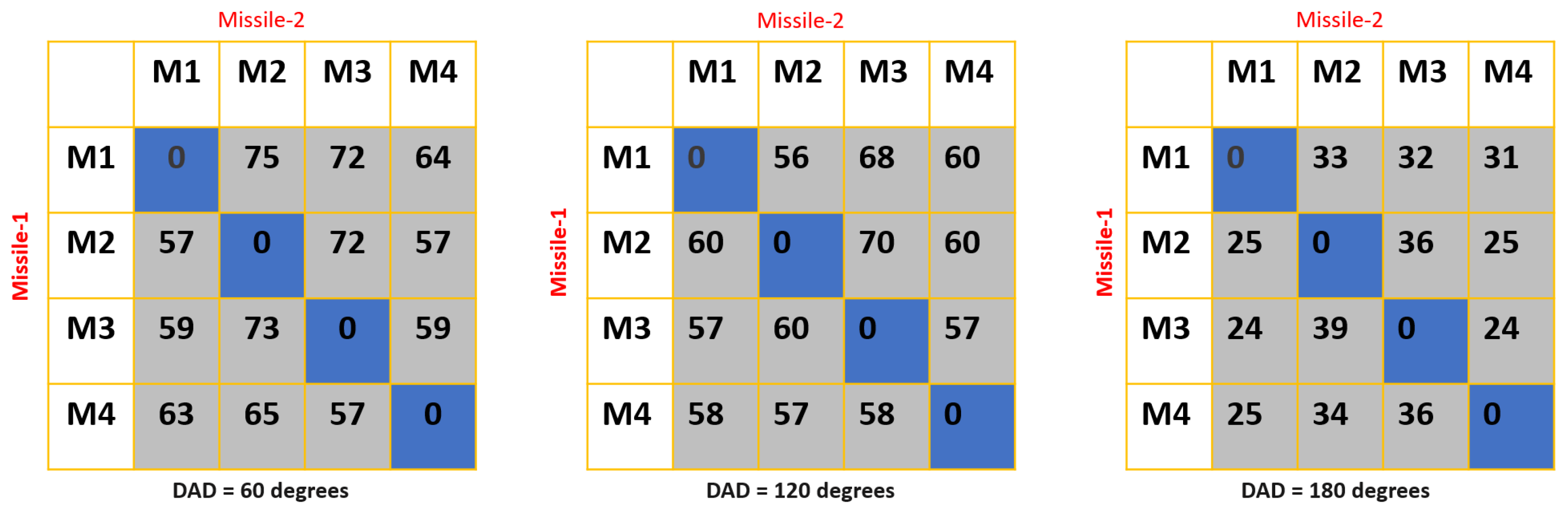
5.1. An Assessment Based on Missile Launch Directions and Varied Decoy Deployment Regions

In each simulation run, each leader decoy in the group moves toward a target point defined by its deployment angle. We aim to evaluate the success rate of the proposed approach with varying missile threat launch directions. To achieve this, we examine three cases based on the deployment angle of each leader decoy. In the first case, the angle difference between the two leader decoys is 60 degrees; in the second case, it is 120 degrees; and in the third case, it is 180 degrees. This allows us to observe how the geometric arrangement of missile threat points and leader decoy positions affects the mission’s success rate.

As seen in Figure 7, when the deployment angle difference between the two leader decoys is 60 degrees, the decoys achieve a mission success rate of up to 75% when one missile is launched from the first direction and the other from the second direction. When the angle difference is 120 degrees, the highest mission success rate is 70%, with one missile launched from the second direction and the other from the third direction. If the angle difference is 180 degrees, the decoys achieve a maximum success rate of 59% when one missile is launched from the second direction and the other from the third direction. It can be inferred that as the difference in deployment angles between leader decoys increases, the mission success rate achieved by the decoys decreases. This decline can be attributed to the geometric relationship between the decoy positions and the target ship point.

Figure 8a,b illustrate scenarios where the three decoys are either positioned on the same side or opposite sides of the protected target, relative to the direction of the incoming missile. We aim to examine how the deployment direction of decoys affects the effectiveness of a decoy deployment strategy in protecting a target ship against a multi-missile threat. As shown in Figure 8a, decoys are deployed in the same direction, with each decoy and the target representing a scattering center. In this context, ESC1 means only decoy1 is activated, ESC2 indicates that both decoy1 and decoy2 are activated, and ESC3 depicts the activation of decoy1, decoy2, and decoy3. It is observed that as the number of activated decoys increases, the ESC point shifts toward the decoys, increasing the probability of the target remaining outside the radar seeker’s field of view. However, when decoys are deployed in the opposite direction, as illustrated in Figure 8b, the situation changes. It is assumed that all assets are within the radar seeker’s field of view. If only decoy1 is activated, ESC1 is positioned along the line connecting decoy1 and the target ship. When decoy2 is also activated, the ESC point shifts toward the target ship. The positions of all ESC points are calculated using Equations (2) and (3) above.

5.2. An Evaluation of the Effectiveness of the Decoy Deployment Strategy with Respect to the Maximum Speed of the Decoys and the Missile Speed

Our objective is to analyze how the maximum speed of the decoys and the missile speed impact the performance of the proposed decoy deployment strategy. To do this, we set a range of maximum decoy speeds at 20, 25, 30, 35, and 40 m/s, and missile threat speeds at 0.7, 0.8, 0.9, 1, and 1.1 Mach.

Table 2. The mission success rate (%) for the MADDPG algorithm [19].

	Missile Speed (in Mach)
Decoy Max Speed	0.7	0.8	0.9	1	1.1
20	65	62	63	64	62
25	65	67	66	68	65
30	64	67	64	66	64
35	63	60	63	66	63
40	60	60	58	60	58

shows the mission success rates achieved by six decoys trained with the MADDPG algorithm, based on the decoy’s maximum speed and the missile speed. When the maximum decoy speed is 25 m/s, the mission success rate is the highest across all missile speeds, with success rates of 65%, 67%, 66%, 68%, and 65%, respectively. The highest mission success rate (68%) is achieved when the decoy’s maximum speed is 25 m/s, and the missile speed is 1 Mach.

Table 3. The mission success rate (%) for the MATD3 algorithm [21].

	Missile Speed (in Mach)
Decoy Max Speed	0.7	0.8	0.9	1	1.1
20	67	63	64	66	66
25	65	64	65	68	67
30	66	68	68	71	68
35	63	64	62	69	64
40	61	58	59	64	61

illustrates the mission success rates achieved with varying decoy maximum speeds and missile speeds, based on decoys trained using the MATD3 algorithm. According to the data, the highest mission success rate of 71% is attained when the decoy’s maximum speed is 30 m/s and the missile speed is 1 Mach. The mission success rate shows an increasing trend from 20 m/s to 30 m/s. However, beyond 30 m/s, the success rate begins to decline.

There is a trade-off between the decoy’s maximum speed and ensuring that the decoys remain within the radar seeker’s field of view (FOV). If the decoys move too quickly, the likelihood of them exiting the radar seeker’s FOV increases, leading to mission failure. Conversely, if the decoys move too slowly, the probability of successfully completing the mission decreases.

To evaluate the impact of the decoy’s maximum speed on mission execution time, we kept certain parameters fixed to ensure a fair comparison. The mission execution time depends on the decoy deployment angles and missile launch direction as well. For this reason, we chose a scenario where the leader decoy in the first cluster is deployed toward decoy deployment region III, and the leader decoy in the second cluster is deployed toward region IV. One missile is launched from direction 1, and the other from direction 2.

As shown in

Table 4. Simulation time with respect to the decoy maximum speed.

	Decoy Maximum Speed (m/s)
	20	25	30	35	40
simulation sample time (st = 0.1 s)	245	249	252	257	260

, as the maximum speed of the decoys increases, the simulation time required to complete the defense mission also increases. This suggests that faster-moving decoys can move further away from the target ship compared to slower decoys. Consequently, higher speeds may increase the miss distance between the real target and missile threats, provided that the decoys remain within the radar seeker’s field of view.

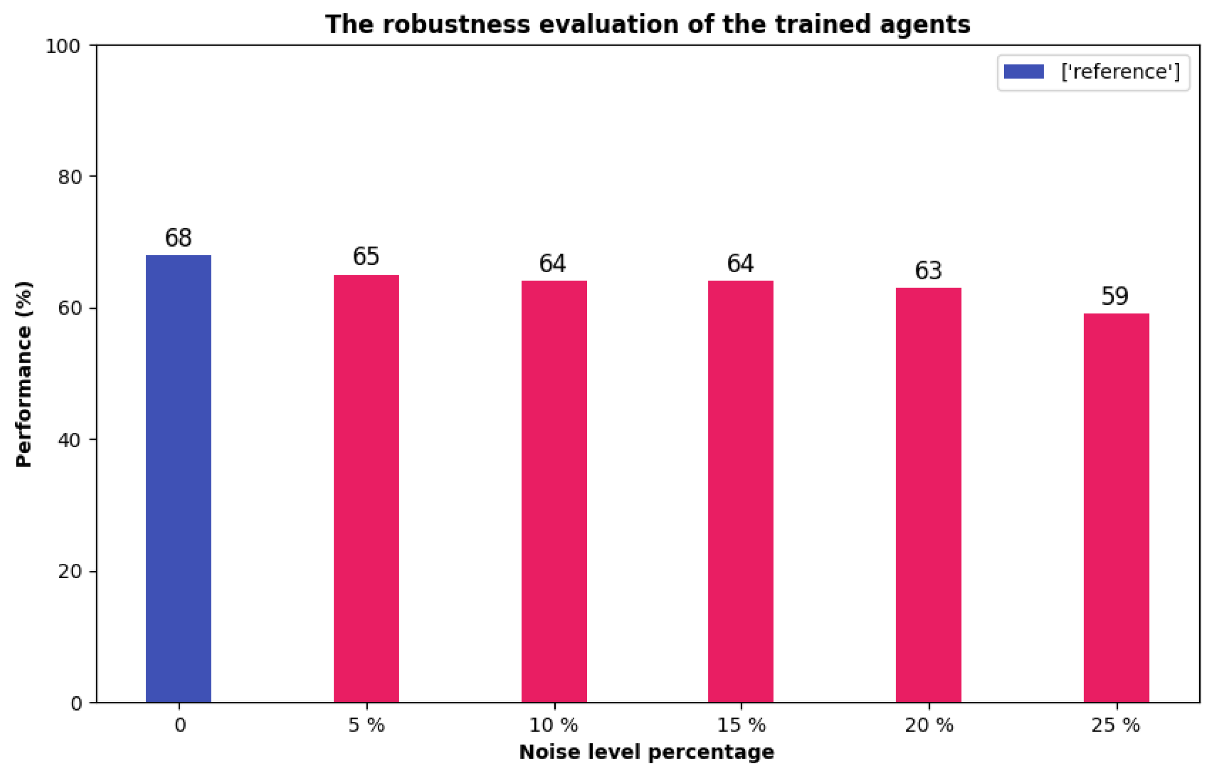
5.3. Robustness Evaluation of Trained Decoys under Noisy Conditions

The observation vector values are derived from sensor data. However, due to imperfections in the sensor readings, the decoys may struggle to perform effectively when exposed to noise. To assess the robustness of the proposed decoy deployment strategy, we introduce varying levels of noise to the observation vector, which is normalized between 0 and 1. The noise values are set as percentages: 5%, 10%, 15%, 20%, and 25%. The observation vector with noise is calculated by adding the nominal observation vector to the product of the noise percentage and the nominal observation.

We use the success rate achieved with zero noise as a reference for a fair comparison. Generally, the success rate decreases as the noise level in the simulation environment increases as illustrated in Figure 9. At a 25% noise level, our proposed deployment strategy shows a 7% drop in performance, reducing the success rate to 59%. Different types of noise functions can be applied to enhance the robustness of the proposed approach.

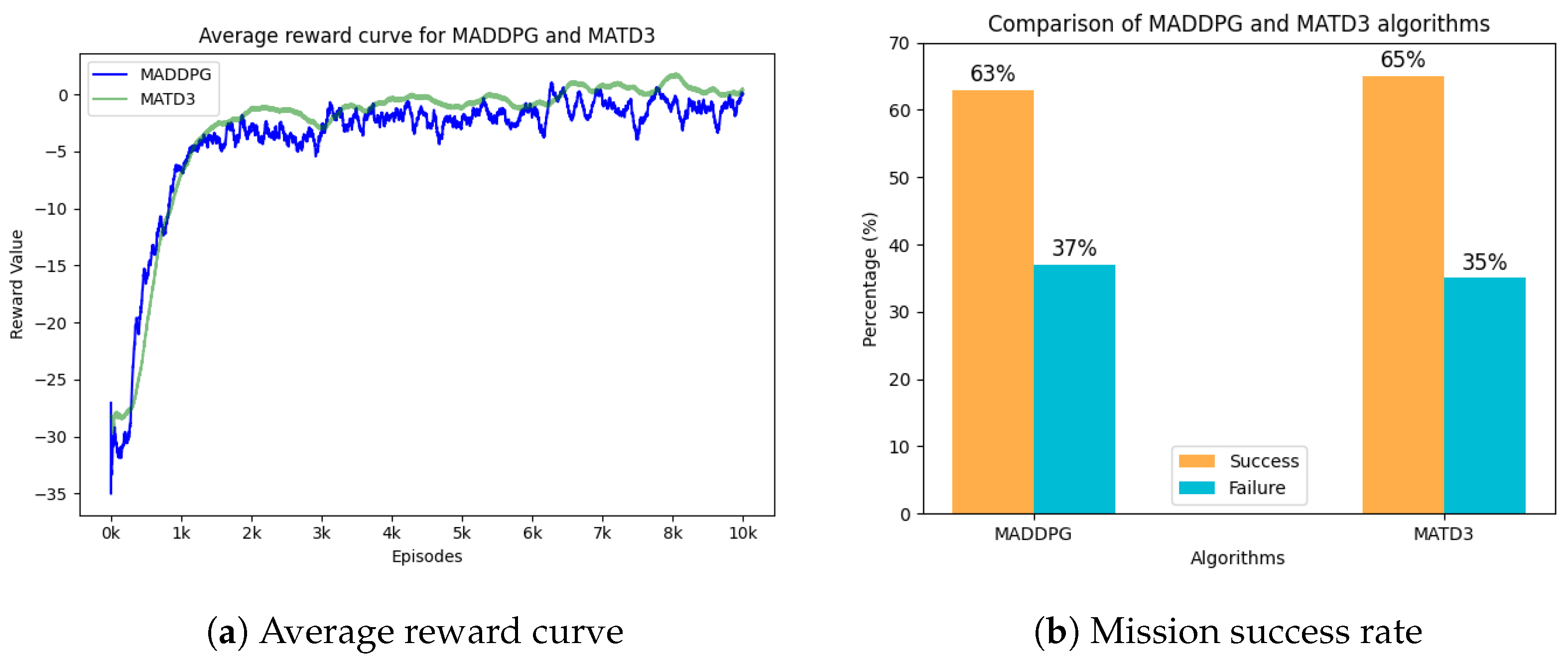
5.4. Comparisons of MADDPG and MATD3 Algorithms

The MADDPG and MATD3 algorithms are used to train the decoys. The performance of the decoys trained with these algorithms is then compared to analyze and evaluate the effectiveness of each algorithm in this type of scenario. Figure 10a illustrates the average reward curve of normalized reward values for the MADDPG and MATD3 algorithms. As shown in the figure, the reward values for MADDPG are generally higher compared to those for MATD3. Figure 10b displays the mission success rates achieved by the MADDPG and MATD3 algorithms. The results show that MADDPG achieves a 63% success rate, while MATD3 achieves a 65% success rate. This indicates that the MATD3 algorithm slightly outperforms the MADDPG algorithm.

6. Conclusions

In this study, we propose a multi-agent reinforcement learning-based decoy deployment strategy designed to enhance the survival probability of a naval platform against salvo missile attacks using six decoys. The scenario involves activating the decoys in two groups, each consisting of three decoys. These groups deploy in a circular formation to achieve their mission.

The decoys are trained separately using the MADDPG and MATD3 algorithms. After training, we evaluate the proposed decoy deployment strategy based on parameters such as decoy deployment angle and maximum decoy speed. Our results demonstrate that decoys deployed on the same side perform better compared to those deployed on opposite sides relative to the target platform. The highest mission success rate achieved using the MADDPG algorithm is 65% when the decoy maximum speed is 25 m/s and the missile speed is 1 Mach. For the MATD3 algorithm, the highest mission success rate is 71%, achieved when the decoy maximum speed is 30 m/s and the missile speed is 1 Mach. Generally speaking, MATD3 slightly outperforms MADDPG, with overall success rates of 63% and 65%, respectively. This improvement is attributed to the fact that decoys trained with MATD3 achieve better formation configurations compared to those trained with the MADDPG algorithm.

Although our approach achieves a high success rate in mission execution, we acknowledge that there are two notable limitations. Firstly, as the noise in the sensor data increases, the performance of the proposed decoy deployment strategy declines. Secondly, the decoys face difficulties in forming the required configuration quickly after deployment, which affects the mission success rate. To address these issues, efforts should be directed toward optimizing hyperparameters and reward coefficients.

References

1. Roome, S. Digital radio frequency memory. Electron. Commun. Eng. J. 1990, 2, 147–153. [Google Scholar] [CrossRef]
2. Kwak, C. Application of DRFM in ECM for pulse type radar. In Proceedings of the 2009 34th International Conference on Infrared, Millimeter, and Terahertz Waves, Busan, Republic of Korea, 21–25 September 2009; IEEE: Piscataway, NJ, USA, 2009; pp. 1–2. [Google Scholar]
3. Davidson, K.; Bray, J. Understanding digital radio frequency memory performance in countermeasure design. Appl. Sci. 2020, 10, 4123. [Google Scholar] [CrossRef]
4. Javed, H.; Khalid, M.R. A novel strategy to compensate the effects of platform motion on a moving DRFM jammer. In Proceedings of the 2021 International Bhurban Conference on Applied Sciences and Technologies (IBCAST), Islamabad, Pakistan, 12–16 January 2021; IEEE: Piscataway, NJ, USA, 2021; pp. 956–960. [Google Scholar]
5. Mears, M.J. Cooperative electronic attack using unmanned air vehicles. In Proceedings of the 2005, American Control Conference, Portland, OR, USA, 8–10 June 2005; IEEE: Piscataway, NJ, USA, 2005; pp. 3339–3347. [Google Scholar]
6. Mears, M.J.; Akella, M.R. Deception of radar systems using cooperatively controlled unmanned air vehicles. In Proceedings of the 2005 IEEE Networking, Sensing and Control, Tucson, AZ, USA, 19–22 March 2005; IEEE: Piscataway, NJ, USA, 2005; pp. 332–335. [Google Scholar]
7. Ilaya, O.; Bil, C.; Evans, M. Distributed and cooperative decision making for multi-UAV systems with applications to collaborative electronic warfare. In Proceedings of the 7th AIAA ATIO Conf, 2nd CEIAT Int’l Conf on Innov and Integr in Aero Sciences, 17th LTA Systems Tech Conf, Belfast, Northern Ireland, 18–20 September 2007; Followed by 2nd TEOS Forum. p. 7885. [Google Scholar]
8. Akhil, K.; Ghose, D.; Rao, S.K. Optimizing deployment of multiple decoys to enhance ship survivability. In Proceedings of the 2008 American Control Conference, Seattle, WA, USA, 11–13 June 2008; IEEE: Piscataway, NJ, USA, 2008; pp. 1812–1817. [Google Scholar]
9. Vermeulen, A.; Maes, G. Missile avoidance maneuvres with simultaneous decoy deployment. In Proceedings of the AIAA Guidance, Navigation, and Control Conference, Chicago, IL, USA, 10–13 August 2009; p. 6277. [Google Scholar]
10. Chen, Y.M.; Wu, W.Y. Cooperative electronic attack for groups of unmanned air vehicles based on multi-agent simulation and evaluation. Int. J. Comput. Sci. Issues 2012, 9, 1. [Google Scholar]
11. Kwon, S.J.; Seo, K.M.; Kim, B.s.; Kim, T.G. Effectiveness analysis of anti-torpedo warfare simulation for evaluating mix strategies of decoys and jammers. In Proceedings of the Advanced Methods, Techniques, and Applications in Modeling and Simulation: Asia Simulation Conference 2011, Seoul, Republic of Korea, 16–18 November 2011; Proceedings. Springer: Berlin/Heidelberg, Germany, 2012; pp. 385–393. [Google Scholar]
12. Jeong, J.; Yu, B.; Kim, T.; Kim, S.; Suk, J.; Oh, H. Maritime application of ducted-fan flight array system: Decoy for anti-ship missile. In Proceedings of the 2017 Workshop on Research, Education and Development of Unmanned Aerial Systems (RED-UAS), Linköping, Sweden, 3–5 October 2017; IEEE: Piscataway, NJ, USA, 2017; pp. 72–77. [Google Scholar]
13. Shames, I.; Dostovalova, A.; Kim, J.; Hmam, H. Task allocation and motion control for threat-seduction decoys. In Proceedings of the 2017 IEEE 56th Annual Conference on Decision and Control (CDC), Melbourne, Australia, 12–15 December 2017; IEEE: Piscataway, NJ, USA, 2017; pp. 4509–4514. [Google Scholar]
14. Dileep, M.; Yu, B.; Kim, S.; Oh, H. Task assignment for deploying unmanned aircraft as decoys. Int. J. Control. Autom. Syst. 2020, 18, 3204–3217. [Google Scholar] [CrossRef]
15. Jiang, D.; Zhang, Y.; Xie, D. Research on cooperative radar jamming effectiveness based on drone cluster. In Proceedings of the International Conference on Electronic Information Technology (EIT 2022), Chengdu, China, 18–20 March 2022; SPIE: Bellingham, DC, USA, 2022; Volume 12254, pp. 339–344. [Google Scholar]
16. Conte, C.; Verini Supplizi, S.; de Alteriis, G.; Mele, A.; Rufino, G.; Accardo, D. Using drone swarms as a countermeasure of radar detection. J. Aerosp. Inf. Syst. 2023, 20, 70–80. [Google Scholar] [CrossRef]
17. Bildik, E.; Yuksek, B.; Tsourdos, A.; Inalhan, G. Development of Active Decoy Guidance Policy by Utilising Multi-Agent Reinforcement Learning. In Proceedings of the AIAA SCITECH 2023 Forum, Online, 23–27 January 2023; p. 2668. [Google Scholar]
18. Kim, K. Engagement-Scenario-Based Decoy-Effect Simulation Against an Anti-ship Missile Considering Radar Cross Section and Evasive Maneuvers of Naval Ships. J. Ocean. Eng. Technol. 2021, 35, 238–246. [Google Scholar] [CrossRef]
19. Lowe, R.; Wu, Y.I.; Tamar, A.; Harb, J.; Pieter Abbeel, O.; Mordatch, I. Multi-agent actor-critic for mixed cooperative-competitive environments. Adv. Neural Inf. Process. Syst. 2017, 30. [Google Scholar]
20. Lillicrap, T.P.; Hunt, J.J.; Pritzel, A.; Heess, N.; Erez, T.; Tassa, Y.; Silver, D.; Wierstra, D. Continuous control with deep reinforcement learning. arXiv 2015, arXiv:1509.02971. [Google Scholar]
21. Ackermann, J.; Gabler, V.; Osa, T.; Sugiyama, M. Reducing overestimation bias in multi-agent domains using double centralized critics. arXiv 2019, arXiv:1910.01465. [Google Scholar]
22. Fujimoto, S.; Hoof, H.; Meger, D. Addressing function approximation error in actor-critic methods. In Proceedings of the International Conference on Machine Learning, Stockholm, Sweden, 10–15 July 2018; PMLR. pp. 1587–1596. [Google Scholar]
Figure 1. Envisioned simulation environment.
Aerospace 11 00799 g001
Figure 2. Missile-target engagement.
Aerospace 11 00799 g002
Figure 3. Reinforcement learning process.
Aerospace 11 00799 g003
Figure 4. Centralized training and decentralized execution framework.
Aerospace 11 00799 g004
Figure 5. Decoy deployment regions and angles.
Aerospace 11 00799 g005
Figure 6. Leader–follower formation configuration and the relative position of leader agent with the desired point.
Aerospace 11 00799 g006
Figure 7. Mission success percentage (%) based on the missile launch directions and differences in deployment angles (DAD) for each decoy group. (Obtained by MADDPG algorithm).
Aerospace 11 00799 g007
Figure 8. Deployment direction impacts of multiple decoys on the equivalent scattering center (ESC) point.
Aerospace 11 00799 g008
Figure 9. The impact of noise on the mission success rate.
Aerospace 11 00799 g009
Figure 10. Average reward curve and mission success rate for MADDPG and MATD3 algorithms.
Aerospace 11 00799 g010