Pulsar Signal Adaptive Surrogate Modeling

Abstract

As the number of spacecraft heading beyond Earth’s orbit increased in recent years, autonomous navigation solutions have become increasingly important. One such solution is pulsar-based navigation. The availability of pulsar signals for simulations and HIL testing is essential for the development of pulsar-based navigation. This study proposes a method to develop a surrogate model of pulsar signals based on radio pulsar observations. The selection of suitable pulsars for the radio telescope is discussed, and a series of observations are conducted. The collected data are processed using the PRESTO software, and the pulsar parameters for the model are derived. Unlike current pulsar signal models, the proposed model anticipates pulsar signal parameters to change over time. It can provide dynamic input parameters for known synthetic pulsar signal generators, resulting in a more realistic signal.

1. Introduction

The majority of space missions to date have targeted either the Earth’s orbit or the inner Solar System with only a fraction of spacecraft sent further from the Sun. There are five NASA-led missions currently approaching the outer limits of the Solar System and entering the interstellar medium. The farthest man-made object from Earth is currently (as of July 2024) Voyager 1 (https://voyager.jpl.nasa.gov/mission/status/, accessed on 6 October 2024) with a distance of $163.65$ AU ($2.45\times {10}^{10}$ $\mathrm{k}$$\mathrm{m}$), which makes the precision of Earth-based position and distance tracking limited. For parts of the SC trajectory that are far from Earth’s orbits and away from Solar System objects, the range of possible means of navigation is limited. The baseline navigation instrument of the SC is the IMU. Beyond this, most missions now rely on regular communication with the Earth via the DSN to obtain navigation updates and corrections, with necessary processing carried out on the Earth. Due to the DSN tracking limitations, there is a need for novel navigation methods that will complement those currently used and allow for operations in locations outside of the Solar System. The motivation for this work is the use of variable celestial signal sources represented mainly by the X-ray pulsar signals [1,2,3,4] and to innovate the currently used methods for synthetic signal generation in developing XNAV.

The advancement of XNAV algorithms and instruments necessitates the availability of a large amount of synthetic pulsar signals. Current signal generator methods (Section 1.4) share a simplified assumption, that their inputs (pulsar signal parameters) are derived as constant values without evolution in time being the common practice originating from long observations conducted with the best available observatories. In practice, due to the effect of ISM instabilities and a significantly reduced pulsar signal sensor sensitivity on-board of an SC, both of the assumptions lose validity. In this work, the authors propose a method for dynamic synthetic pulsar signal generation using a surrogate model based on own pulsar observations with all parameters evolvable in the time domain. For a comparison between the common and proposed assumptions on pulsar signal time evolution, see Figure 1.

1.1. Physics of Pulsars

Pulsars are highly magnetized neutron stars that emit electromagnetic radiation out of their magnetic poles with the so-called lighthouse effect due to their unaligned magnetic and rotational axis [5,6]. The radiation covers a wide range of spectra for most pulsars containing optical, radio, X-ray, and $\gamma$-ray wavebands. The geometry of a single pulse is studied in detail in [7].

The pulsar pulse period increases with time due to the loss of angular kinetic energy. The rate of increase is often marked as $\dot{P}$ and is one of the important quality parameters of pulsar’s suitability for navigation purposes. There are two main types of pulsars concerning navigation purposes. Normal pulsars, which are characterized by $P\sim$ $0.5$ $\mathrm{s}$ and $\dot{P}\sim$ $\mathrm{e}-15$ $\mathrm{s}$/$\mathrm{s}$, and millisecond pulsars having $P\sim$ 3 $\mathrm{m}$$\mathrm{s}$ and $\dot{P}\sim$ $\mathrm{e}-20$ $\mathrm{s}$/$\mathrm{s}$. Millisecond pulsars are generally more stable as many of them are binary systems, where the consumed energy is mostly taken from the companion objects and not from the neutron star rotation. Approx. $80\%$ millisecond pulsars contain a counterpart in a binary system, while normal pulsars are part of a binary system only in less than $1\%$ [8].

In pulsar data processing, one needs to consider the effects beyond the pulsar itself being a signal source, but also the effects caused by the medium between the source pulsar and the receiver. For space applications, this means the ISM, and for Earth-based applications, the effect of the atmosphere needs to be applied as well. Traveling through the ISM, there are three effects that modify the signal: dispersion, scintillation, and scattering [9].

The ISM inhomogeneities and their change in time mean there are different distances for the pulsar signal to travel within the ISM [10]. This can cause delays in time relative to signal traveling shorter paths. The resulting pulse scattering greatly decreases the timing results. The timescale for changes in pulsar signal due to turbulent ISM ranges from minutes to weeks and, depending on the observation length, may or may not be averaged out in resulting pulsar profile characteristics.

1.2. Surrogate Modeling

A surrogate model helps in the situation when either the internal principles are not known and it is not possible to perform a sufficient amount of experiments due to their time complexity or cost, or if the inner mechanism is known, the evaluation of the equations describing the physics behind is too complex and slow for the simulation to be run in a reasonable time [11]. This way it is used either to save computational time or to deal with a small number of samples. Examples of surrogate modeling techniques include Support Vector Machines [12], GPR [13,14], Multivariate Simplex Splines [15] or Artificial Neural Networks [16].

In space-related modeling [17], the surrogate model can be an advantageous technique as physical models can be highly complex, even in domains where most of the included phenomena can be described. The utilization of surrogate techniques in the modeling of time series and possible problems and their mitigation is discussed in [18]. Surrogate modeling with GP was used to lower the cost of candidate period evaluation as an optimization in the pulsar period search process [19]. Pulsar models have also been used to test new gravity theories [20] or to model the light curve of pulsar mergers [21].

The main difficulty in the application of the surrogate model technique is the need to select a proper model class. Several authors tried to devise generic methods to solve this [22,23]. Another problem to be resolved is the selection of sampling points to be evaluated in the construction of the surrogate model [24]. With complex systems, a single surrogate model may not be able to authentically represent the system’s behavior. In that case, either a combination of surrogate models or a hybrid combination of surrogate and full models can be used [25]. Another approach in complex system’s surrogate modeling is to describe an adaptive surrogate model that can describe regions of modeled state space, where the model measure of accuracy is out of the required limits [26,27]. For these regions, different surrogate model classes can be used, weights of multiple surrogate models can be adjusted, or additional sampling points can be requested.

GPR is a non-parametric regression technique for surrogate modeling applying the Bayes theorem to a distribution of functions [14,28,29]. With this method, several priors on the functions that should fit target data are established first: a mean, a variance, and a degree of smoothness for the given length scale. Next, the observed data points are used together with their noise level. Using the Bayes theorem, a new posterior distribution of functions can be obtained. The posterior distribution of functions will have the mean value passing through the data used for training. Variance can be used to identify confidence intervals for given and newly predicted data points. General utilization of surrogate techniques, including GP for surface modeling, can be found in [30].

The two components of GP are the mean function, which can be used to implement some prior knowledge about the resulting system being modeled, and the covariance (kernel) function measuring the similarity of each input point. Among the commonly used kernel functions are SEK, also known as Gaussian kernel [31], Matérn kernel, ESSK and RQK [16,29]. Kernels can also be combined together if necessary. Different kernels or the same kernels with different parameters can be multiplied and summed to model more complex input data behavior in the model.

One known problem of GPR is its computational complexity being $\mathcal{O}\left(n^3\right)$. For real use, the limit number of input samples lies around $n\sim$ 10,000. If the input dataset to be used for training is bigger or is increasing with time, some techniques to deal with the increasing computational resources required have to be used. Methods for sampling training sets are described in [18,24,26,32].

1.3. Pulsar Navigation and Timing

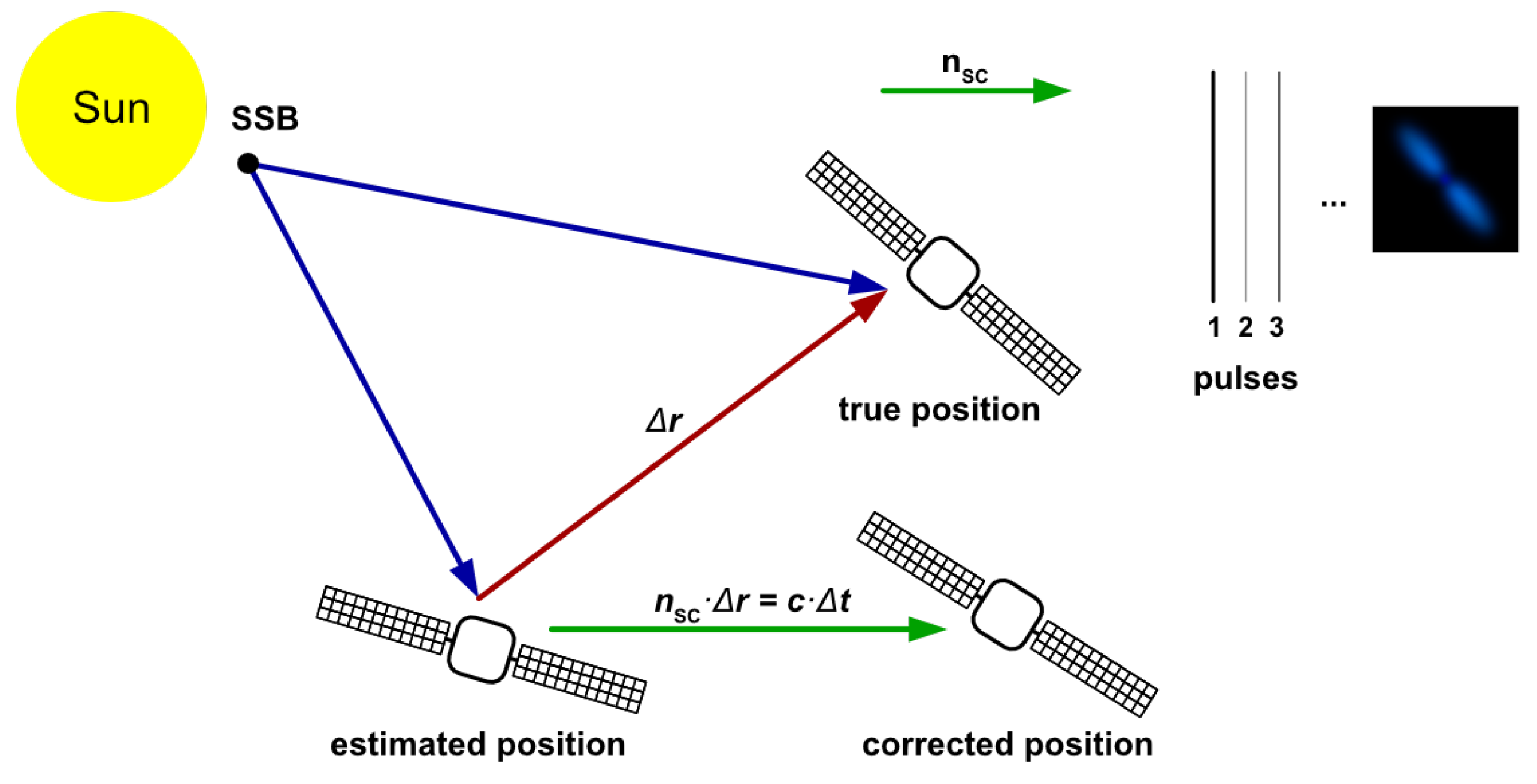
The whole XNAV system scheme consists of two primary elements—the SC and a set of pulsars. As can be seen in Figure 2, the corrected SC position in the direction towards used pulsar $n_{sc}·\Delta r$ equals the speed of light times the measured time difference $c·\Delta t=c·(t_{SSB}-t_{SC})$. A review of the current state of pulsar-based navigation is provided in [33].

For space navigation applications, the X-ray is preferable mainly because the size of the X-ray payload is much smaller compared to the radio payload, while the usability of radio pulsars for navigation is studied in [35]. For other spectral bands, there is only a limited amount of known pulsars which emit signals in visible and $\gamma$-ray parts of the electromagnetic spectrum [36].

Once a detector captures individual photons and marks their TOA in the proper time, the TOA is further processed to reconstruct the pulsar pulse profile and to obtain its signal phase given the observation start. A commonly used processing method is epoch folding [3,8,36]; other methods are devised to increase the performance or detection capabilities [19,37,38,39,40,41].

If a precise pulse period is not known, the search needs to precede the application of epoch folding or similar methods for signal-phase estimation.

Assuming observation time $T_{obs}$ consisting of $N_p$ pulsar periods P and subdividing the period P into $N_b$ bins of length $T_b$, each photon number $c_j\left(T_i\right)$ is folded into ith bin in the jth period. The empirical profile rate function is defined as [36]

$$\tilde{\lambda }\left(T_i\right)={\displaystyle \frac{1}{N_p{T}_b}}\sum _{j=1}^{N_p}{c}_j\left(T_i\right)$$

(1)

The relation of an empirical profile rate function $\tilde{\lambda }\left(T_i\right)$ and real rate function $\lambda \left(T_i\right)$ is introduced in [36]. Having the empirical rate function, different methods (e.g., cross-correlation) can be used to compare it with the pulse profile template ${\lambda }^{\prime }\left(T_i\right)$ to obtain the initial pulse phase. In current methods, the template ${\lambda }^{\prime }\left(T_i\right)$ is created from long-term observations as a close approximation of real rate function $\lambda \left(T_i\right)$. In this work, the proposed approach abandons these traditional assumptions.

The output of epoch folding is a single-pulse TOA. There are different methods for deriving the SC position using the information from pulse TOA. The state-of-the-art differential method transforms the measured-pulse TOA to the SSB, a fixed common point in the inertial coordinate frame, for comparison with the pulsar timing model output. Transforming the measured-pulse TOA to the SSB is known as the time-transfer model [8,42]. The method for large-distance SSB transfers is developed in [43].

Once the time difference between $t_{SC}$ and $t_{SSB}$ has been obtained, it can be used to evaluate the SC’s distance to SSB. The difference between predicted and actual pulse’s TOA gives a relative correction of SC distance to be further used to update the predicted SC position in the next iteration of the navigation algorithm. Based on the number of pulsars used, one can either correct the position in one direction, usually perpendicular to other means of position determination such as DSN. With three pulsars available, one can correct the SC’s 3D position, while with four pulsars, one can obtain precise timing information along with SC’s 3D position. More than four pulsars are used to enable the detection of pulsar signal glitches, scintillation, and other disturbances, and shorten the position fix time using pulses with different periods.

Several published pulsar databases originating from previous research projects are listed in [44,45,46,47]. The advantage of the SEXTANT database (11 pulsars) [47] is that raw data are available through the NICER database of the NASA HEASARC project [48] together with the data processing software. A proper selection of pulsars used and their effects on the initial state estimation is described in [49].

Pulsar navigation is subject to different errors. Some of them can be eliminated using error estimation techniques for time-transfer model errors, SSB position error, pulsar angular position error, pulsar distance error, pulsar proper motion error, and SC clock error. Some errors are caused by changes in ISM, pulsar behavior, and other sources that cannot be influenced nor predicted exactly. The reported positioning precision achieved during simulations and experiments ranges from 100 $\mathrm{m}$ [34,42] to 5 $\mathrm{k}$$\mathrm{m}$ [36,50]. Some authors address precision improvements also with changes to navigation algorithms [51]. The application with a limited pulsar observation time is introduced in [52].

1.4. Pulsar Signal Models

As X-ray pulsar signals cannot be detected on the ground due to the Earth atmosphere’s almost-zero transparency to the X-ray part of electromagnetic spectra and their acquisition through space telescopes is both costly and restrictive to target pulsar selection and the amount of signal obtained, the simulation of X-ray pulsar signals based on their physical characteristics is of great importance for the validation of X-ray pulsar signal processing algorithms, X-ray pulsar-based navigation strategies and physical sensors or whole payload testing [53].

Current signal modeling methods start with the best-measured pulse profile $h\left(\varphi \right)$ fitting to $h^{*}\left(\varphi \right)$. Usually, the fitted profile $h^{*}\left(\varphi \right)$ is defined as a sum of Gaussian functions:

$$h^{*}\left(\varphi \right)=\sum _{i=1}^C{f}_i\left(\varphi \right)$$

(2)

with $f_i\left(\varphi \right)$ defined as

$$f_i\left(\varphi \right)={\displaystyle \frac{a_i}{\sqrt{2\pi {\delta }_i^2}}}exp-{\displaystyle \frac{{(\varphi -{\mu }_i)}^2}{{\delta }_i^2}}$$

(3)

where $f_i$ is the searched Gaussian component i, and ${\mu }_i$, ${\delta }_i$ and $a_i$ are its mean, variance and scaling factor, respectively. Parameter $\varphi$ is the phase of the pulse. With C being the number of Gaussian functions used for the fitting, the higher the C, the better the fit, but the slower the evaluation.

• The direct method is the baseline method [53]. Using the pulse profile model $h^{*}\left(\varphi \right)$, it is divided into a fixed number N of time bins with length $t_b$ such that $t_{b}N=P$ with P being the pulse profile period. For each bin, the value of $h_i^{*}\left(\varphi \right)$, $i\in [1,N]$ is then used as the input parameter for the non-homogeneous Poisson process to generate the number of photons in this bin based on the Poisson distribution.
• The inverse mapping method is introduced in [54]. It is proven that the next photon TOA $t_{n+1}$ can be generated based on the current photon TOA $t_n$. The advantage is that the computational time to generate the signal does not depend on its length but only on the number of generated photons.
• The statistical method from [55] eliminates the direct dependency on observation time and calculations of differential equations for each photon as required by the inverse mapping method. It proves that the probability distribution of photon TOA can be used as the pulse profile during one period. Apart from computational efficiency, the signal and noise are generated separately, allowing for precise control of both.

Other signal modeling methods include the Monte Carlo-based approach proposed in [56], the scale transforming method from [57], and the signal simulation on SC described in [58].

2. Materials and Methods

2.1. Pulsar Visibility

The visibility of an object on the celestial sphere is given by the position of the observer on the Earth’s surface given by latitude $\phi$ and longitude $\lambda$, the coordinates of the object given by declination $\delta$ and right ascension $\alpha$, and the time of observation given by the local hour angle H. Neglecting the difference between the sidereal and universal time, which is $4\min$ per day, the total time above the altitude h is $2H$ [59]. An object rises above the angle h if

$$\delta \ge \phi +h-{90}^{\circ }$$

(4)

For the radio telescope used with $\phi =49°54.514\prime$ and $h={15}^{\circ }$, this gives us minimal declination $\delta =-{25.09}^{\circ }$. For timing and navigation purposes, the measurement window for a single object has to be large enough with a minimum set to be $t_{min}=1 \mathrm{h}$. An observation lasting at least $t_{min}=3600\mathrm{s}$ with angle h above ${15}^{\circ }$ gives us local hour angle $H={7.5}^{\circ }$. For 3600 $\mathrm{s}$ observation duration requirement the declination is $\delta \ge -{24.79}^{\circ }$, for 7200 $\mathrm{s}$ it is $\delta \ge -{23.90}^{\circ }$. For observation planning, the visibility data for each target pulsar are generated.

2.2. Pulsar Radio Flux Intensity

To obtain an accurate-pulse TOA estimate, the high signal flux density is crucial to obtain a high SNR. As the flux density varies with the receiver’s frequency range, the total flux of the pulsar in this range needs to be analyzed. For most pulsars, the general rule is the higher the observing frequency, the lower the flux density. As noted in [60,61], the vast majority of known pulsars’ spectral characteristics fit into a few well-described types:

• Simple power-law spectrum;
• Broken power-law spectrum;
• Log parabolic spectrum;
• Power law with high-frequency cut-off;
• Power law with low-frequency turn-over.

Apart from these generic models, a particular class named GPSP is known [62,63,64], containing around 30 pulsars.

Another factor that needs to be considered is that the flux of individual pulsar is not constant in time. This is caused by a combination of fluctuations in the pulsar emissions itself and diffractive and refractive interstellar scintillation [65,66]. Ref. [67] showed that pulsars in large distances with high DM are more stable with respect to these changes. From the measurements and simulations using the NE2001 galaxy model, Ref. [61] concludes that the maximal effect of these fluctuations should be related to a maximal modulation index of $0.3$.

The radio receiver used for our experiments is described in Section 2.4 and [68]. It operates in the range from 1.0 $\mathrm{G}$$\mathrm{Hz}$–2.0 $\mathrm{G}$$\mathrm{Hz}$. To obtain the radio telescope’s overall flux, the exact parameters for a given spectral type of each pulsar need to be determined. Consequently, the known flux intensity is integrated over the radio telescope spectrum range. The authors started with the ATNF pulsar catalogue (https://www.atnf.csiro.au/people/pulsar/psrcat/, accessed on 6 October 2024) version 2.0.1, and applied the following steps for each pulsar:

• For pulsars without a spectral index listed in the catalog with only a single measurement, assume $\alpha =-1.6$ based on [61,69].
• For pulsars with two or more measurements, evaluate the index from these measurements.
• Data from available papers are used to add or replace the spectral index and flux data with more precise values. Data from [60,70] are already part of ATNF version 2.0.1 and higher, so there is no need for a special evaluation. For [61], data are also part of ATNF, but it is possible to utilize this paper’s classification and extra information. Other references utilized in this step include [63,64].
• For each pulsar and each of its measurements, compute the total flux.
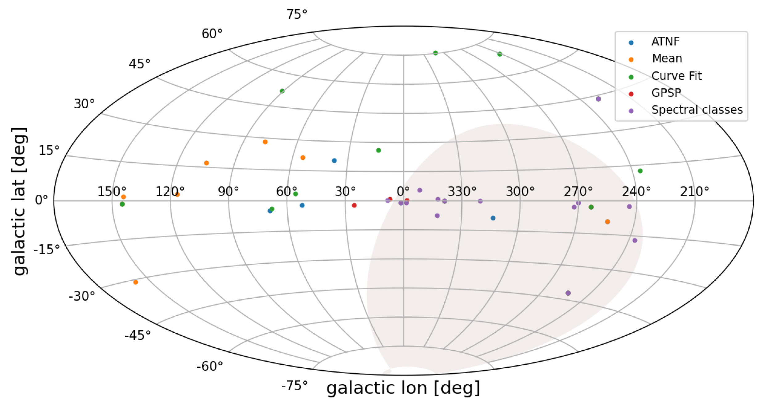
• Sort pulsars according to their total expected flux for the used radio telescope. The pulsar distribution in galactic coordinates can be seen in Figure 3 with point colors based on the method used to compute the total flux.

2.3. Observation Planning

Putting all the above information together, an observation plan starting 2024-01-01 and being valid until 2024-12-31 was prepared, containing the 10 best observation candidates as summarized in

Table 1. Observation-related information for the 10 best pre-selected pulsars.

Pulsar	P [s]	Flux [W/m2]	Fl. err [W/m2]	Vis [h]	Close to Sun
J0341+5711	$1.8880$	$9.8358\times {10}^{-10}$	$6.4925\times {10}^{-17}$	all	–
J2043+7045	$0.5880$	$1.5597\times {10}^{-11}$	$3.9111\times {10}^{-19}$	all	–
J0302+2252	$1.2072$	$9.6537\times {10}^{-12}$	$6.9157\times {10}^{-20}$	∼12 h	2024-04-20–05-29
B0818-13	$1.2381$	$4.3899\times {10}^{-12}$	$1.3474\times {10}^{-10}$	∼ 6 h	–
J2352+65	$1.1640$	$3.1631\times {10}^{-12}$	$7.0428\times {10}^{-19}$	all	–
B1642-03	$0.3877$	$3.0014\times {10}^{-12}$	$2.1748\times {10}^{-11}$	∼ 8 h	2024-11-25–12-08
B2016+28	$0.5580$	$2.4174\times {10}^{-12}$	$8.0023\times {10}^{-12}$	∼14 h	–
B1257+12	$0.0062$	$2.2272\times {10}^{-12}$	$1.1490\times {10}^{-11}$	∼11 h	2024-09-22–10-10
B0329+54	$0.7145$	$1.9561\times {10}^{-12}$	$1.8715\times {10}^{-12}$	∼22 h	–
B0950+08	$0.2531$	$1.7966\times {10}^{-12}$	$3.5863\times {10}^{-12}$	∼10 h	2024-09-09–08-01

P is pulsar signal period; Flux is the expected value of flux based on previous evaluations with expected error; Vis is basic per day visibility of the pulsar above horizon; Close to Sun is time; when the pulsar is closer than ${20}^{\circ }$ to the Sun it should not be observed.

.

From these candidates, only PSR B1642-03 has a slightly higher galactic background noise signal, while the rest are in low-noise regions. Another aspect that needs to be considered is pulsar period duration with respect to the time resolution of the radio telescope used. Based on the Nyquist–Shannon sampling theorem and time resolution of 1 $\mathrm{m}$$\mathrm{s}$ for recorded spectrum, it is possible to observe pulsars with at least a 2 $\mathrm{m}$$\mathrm{s}$ period. The pulsar with the shortest period from our pre-selected pulsars is PSR B1257+12 with a period of $6.2$ $\mathrm{m}$$\mathrm{s}$. All other pulsars have their periods an order of magnitude higher.

2.4. Radio Telescope Characteristics

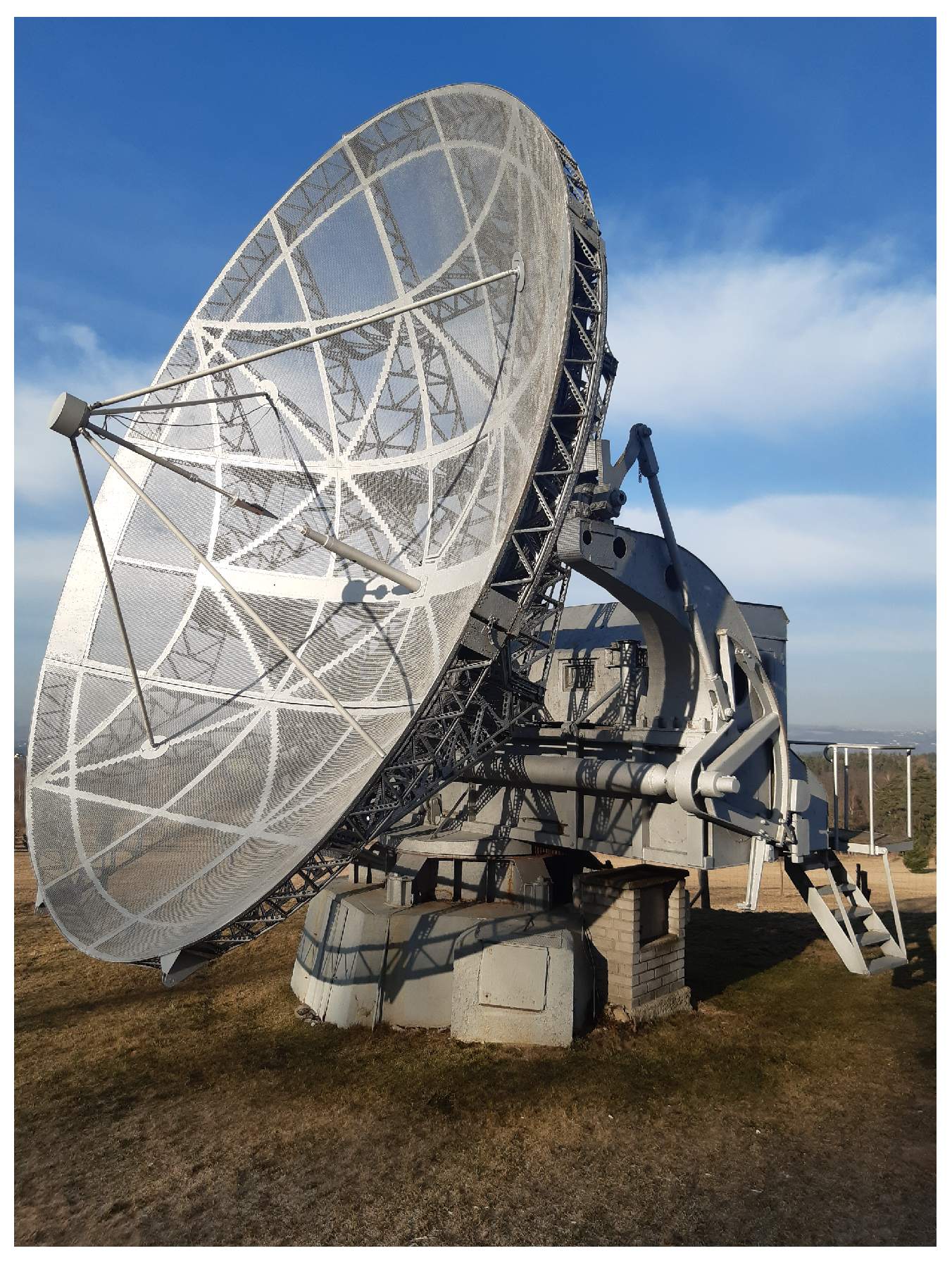
The radio telescope used in this work [68] is part of equipment built for the Sun observations by Astronomical Institute of the CAS. Radio telescope RT2 as seen in Figure 4 is based on the German Würzburg-Riese RADAR antenna and platform later equipped with new radio parts. Since 1994, RT2 has been used mainly for tests, short-term experiments, and the development of new observation instruments. The basic parameters are in

Table 2. RT2 Basic parameters.

parabolic reflector, diameter	$7.5$ $\mathrm{m}$
bearing pointing accuracy	${0.05}^{\circ }$
half power beam width	${1.0}^{\circ }$ to ${2.0}^{\circ }$
frequency range	1.0 $\mathrm{G}$$\mathrm{Hz}$ to 2.0 $\mathrm{G}$$\mathrm{Hz}$
4 sub-bands with 250 $\mathrm{M}$$\mathrm{Hz}$ each	SP1, SP2, SP3, SP4
spectral channels per sub-band	1024
frequency spectral resolution	303 $\mathrm{k}$$\mathrm{Hz}$
time resolution	1 $\mathrm{m}$$\mathrm{s}$
dynamic range	50 $\mathrm{d}$$\mathrm{B}$
ADC resolution	$14\mathrm{bits}$
mechanical limits for antenna	elevation: ${10.0}^{\circ }$ to ${84.0}^{\circ }$, azimuth: ${1.0}^{\circ }$ to ${357.0}^{\circ }$

.

2.5. Pulsar Signal Model Requirements and Design

For pulsar timing and navigation solutions, HIL testing or studies using simulations, there is a crucial need for the ability to produce tens of hours-long pulsar signals for a high number of pulsars simultaneously. One option is to replay real signals from space-based X-ray telescopes like Chandra (https://www.nasa.gov/mission/chandra-x-ray-observatory/, accessed on 6 October 2024), XMM-Newton (https://sci.esa.int/web/xmm-newton/, accessed on 6 October 2024) or NICER (https://heasarc.gsfc.nasa.gov/docs/nicer/, accessed on 6 October 2024). The second option is to generate a synthetic sequence using pulsar signal generators (see Section 1.4).

The challenge of using real signals measured in space is mainly the inability to select pulsars of one’s own choice. Still, even for pulsars observed by X-ray telescopes, the amount of data in terms of the number of observations and their length is strictly limited. With current pulsar models, the problem is that the set of pulsar parameters is fixed, and from this perspective, they can model only the short-term behavior of the pulsar signal. These static models are based on the pulsar time and phase model defined by

$$\Phi \left(t\right)=\Phi \left(t_0\right)+\sum _{n=0}^{n=+\infty }{\displaystyle \frac{1}{n!}}{f}^{\left(n\right)}{(t-t_0)}^{n+1}$$

(5)

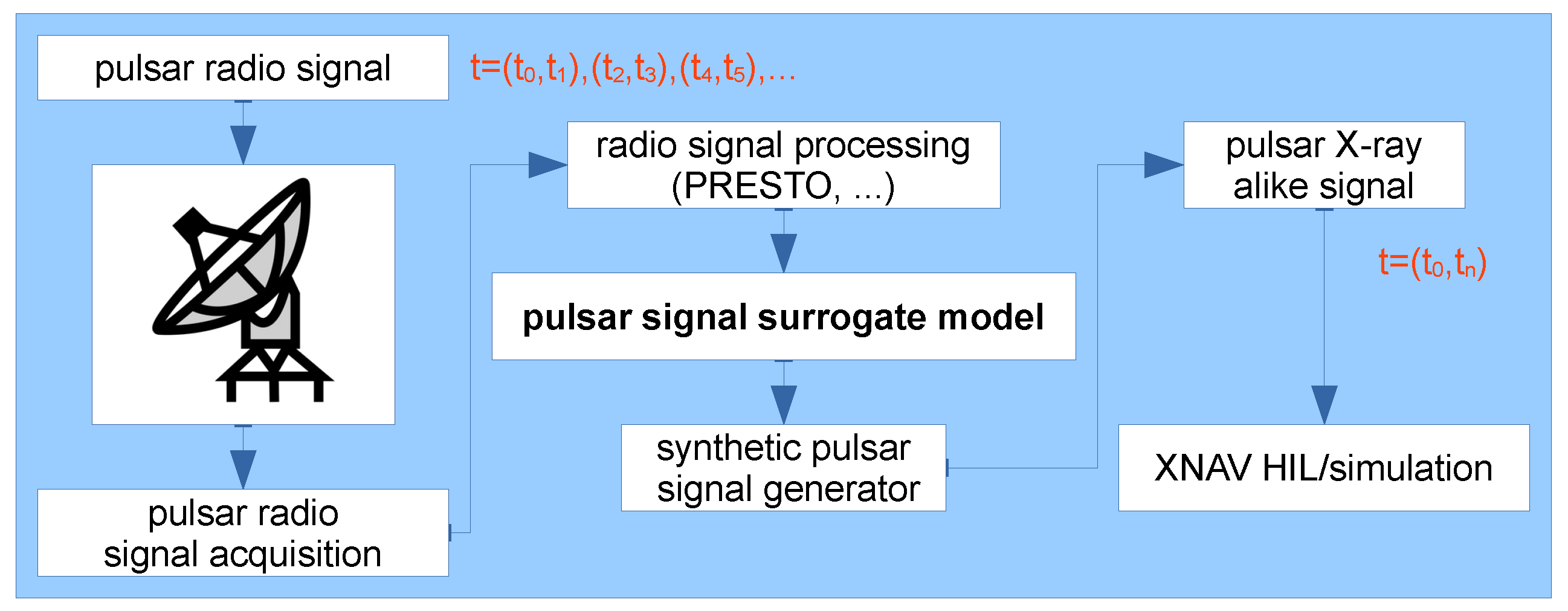
where $f\left(t\right)=f_s\left(t\right)+f_d\left(t\right)$ is real pulsar frequency as a combination of source frequency $f_s$ and Doppler frequency shift in moving sensor (SC) $f_d$ [36]. The $f_s$ is expected to be constant with respect to time or have constant the first or second derivatives—period change rate and acceleration. A possible solution evaluated in this work is using the radio part of the electromagnetic spectrum to observe the real signal of pulsars to produce a dynamic pulsar signal model feeding input parameters for the synthetic signal generator to generate an X-ray-like signal. The idea of moving from a static model to a dynamic one is depicted in Figure 5. The scheme of the proposed solution can be seen in Figure 6.

This offers several advantages:

• There are much more radio telescopes on Earth than X-ray observatories in space.
• For the purpose of pulsar signal modeling, the radio telescope does not need to have the ability to observe a single pulse. This leads to the requirement of smaller sensitivity, further widening the number of radio telescopes that can be used to obtain radio signals.
• Using on-Earth telescopes with a smaller pressure for observation time leads to an increased number of possibly longer observations.
• With different PTA projects running for up to 20 years, there is a long history of possible pulsar radio signals to be used with a very long time span.

The contradiction with on-Earth observations is a limited part of the sky observable compared to the space telescopes. The authors propose the following high-level requirements for the model used as an X-ray-like pulsar signal generator for input parameters:

• The model should utilize radio measurements.
• The model should enable the generation of an X-ray-like signal suitable for use in simulations or HIL tests of pulsar-based navigation and timing solutions.
• The model should enable the reproduction of pulsar signals for objects with known changes in pulsar parameters, like binary pulsars or pulsars with trends in period evolution.
• The radio signal input should be 30$\min$–300$\min$ of length per single observation, based on target pulsar’s SNR.
• The frequency of radio observations should be at least once per month considering the pulsar behavior stability.
• The X-ray-like output should be generated for times with radio observations available but also between them.
• The model should enable the reproduction of pulsar signal characteristic changes relevant to expected use, mainly pulse period, intensity, and shape change.
• The model will include not only the pulsar signal but also an additional noise. The mid- and long-term evolution of the noise for each target pulsar should be modeled as well for a more realistic synthetic signal.

2.6. Pulsar Observations

All pulsar observations presented in this paper were made using the RT2 radio telescope in Ondřejov. Observed pulsars are summarized in Table 1. For each pulsar, at least two measurements with a length of 2 $\mathrm{h}$ and at least one measurement with a length of 3 $\mathrm{h}$ were made. The observation schedule is based on pulsar visibility as described in Section 2.3. To test the effect of the availability of longer data, there is a single observation of PSR J0341+5711 with a length of 5 $\mathrm{h}$. Few observations above the three required are available with a shorter duration than 2 $\mathrm{h}$ due to technical issues during recording, usually due to bad antenna pointing.

2.7. Radio Telescope Signal Processing

Processing the measured data with existing software requires their conversion to some commonly supported format. Due to its simplicity, the SIGPROC filterbank format [71] was selected. Data are converted to this format using 32 bit float-type data per single frequency channel value, and metadata from the observation are used to fill the required header.

The processing of radio data in the SIGPROC filterbank format is carried out with the PRESTO software version 12Mar10 (git c0c6e2f2) [72]. The first part of the data analysis creates a mask to mitigate RFI using the rfifind command. Full-frequency channel masking is not used. The accelsearch command is then used to search for possible birdies—periodic interference in the spectra. The main metric for the usability of observation data for given sub-bands SP1, SP2, SP3, or SP4 is the percentage of good versus bad time intervals from rfifind. Data with a small GTI ratio are omitted by dropping the whole sub-band if GTI’s cover is less than 70% of the observation and there are other sub-bands with a higher GTI ratio.

As this is not a search for new pulsars, the target pulse period and DM are known. They are applied to original raw data with RFI and birdie masking using the prepfold command to produce the pulse TOA.

3. Results

3.1. Pulsar Signal Parameters Interpolation

With data measured and preprocessed, a list of pulsar signal parameters per each observation is obtained. There can be several lists per observation if a long observation is divided into sub-observations. The proposed pulsar radio signal model has been used in a synthetic signal generator, where artificial but realistic changes are expected. The model includes not only the pulsar signal but also different kinds of noise ranging from ISM derived noise and its changes to radio telescope-related noise. The proposed model, based on available observations, is defined by a set of four parameters:

• $\left\{T_{0i}\right\}$, $i\in [1,M]$—list of all starts of observations; M is number of observations used [MJD].
• $\left\{{\varphi }_{0i}\right\}$, $i\in [1,M]$—list of all initial pulse phases [1].
• $\left\{P_i\right\}$, $i\in [1,M]$—list of all pulse periods [$ms$].
• $\left\{I_{ij}^{\prime }\right\}$, $i\in [1,M]$, $j\in [1,N_i]$—list of preprocessed intensities for all pulse bins of all observations [1], building a shape of each profile i.

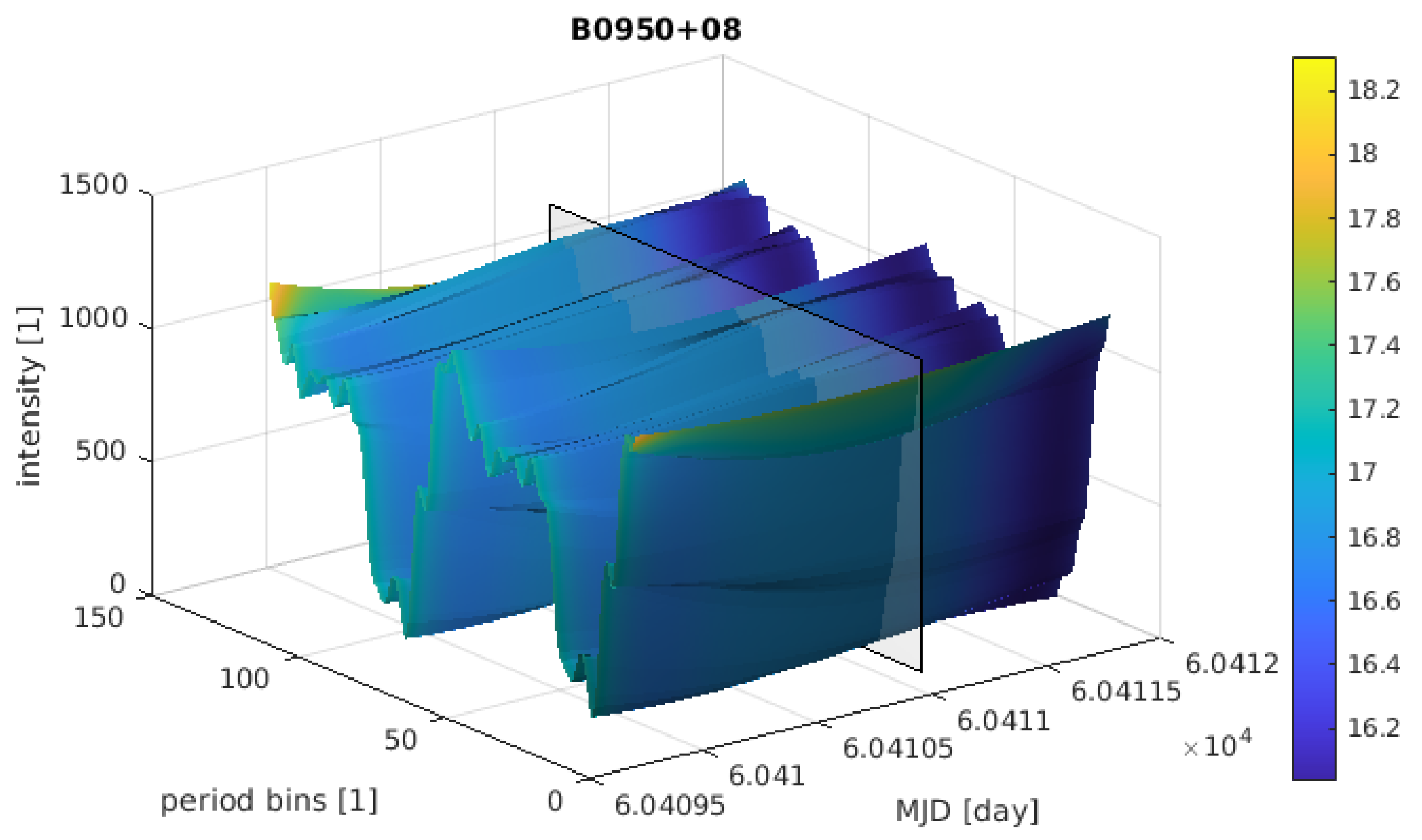
By separating phase and pulse period information, the resulting shape and intensity are not influenced by high-frequency changes in the phase. The model can have the same number of profile bins for different pulsars. For the interpolation or extrapolation method to model the period and shape, it is required to be able to work with a low number of observations M, handle different levels of smoothness of resulting surface in the time and profile shape axis, and have low computational complexity and time for an evaluation of parameters for a given time $T_g$. Speed is crucial for use in synthetic signal generators because there will be a very high number of pulses to be generated. For navigation purposes, computational complexity is less critical due to the lower number of model evaluations, but confidence interval knowledge is crucial. You can see an example of the GPR model in Figure 7.

3.2. Pulsar Signal Generator

In this section, the authors’ own measurements of PSR B0950+08 are used to demonstrate the model buildup and usage for the artificial data generator. PSR B0950+08 can help demonstrate the need for a dynamic pulsar model due to its period evolution [73]. More details about this pulsar and its measurement in radio and X-ray can be found in [74,75]. The difference in the measured pulse profile and mainly its width to published results can be explained primarily by the low SNR of this measurement on the RT2. The pulse profile parameter check has been carried out for other observed pulsars with a higher SNR: PSR B0818-13, J0302+2252, J0341+5711. It should be also noted that there is a systematic error in observations recorded with the RT2 radio telescope, as the resulting period of all pulsars is slightly higher than expected ($+0.07\%$ to $+2.6\%$).

3.2.1. Pulsar Signal Model

As PRESTO sums all partial profiles to obtain an average one, the profile for each observation needs to be normalized by the observation length $L_i$. The profile consists of signals from the target pulsar but also from its surroundings and local Earth-based noise. To remove these from the model, the minimal pulse intensity value $I_{ij}$ of each pulse i is subtracted from the whole pulse, as this should be part of the pulse profile without any or with the minimal signal from the target pulsar:

$$I_{ij}^{\prime }=I_{ij}/L_i-min\left(I_{ij}\right)\forall j\in [1,N_i]$$

(6)

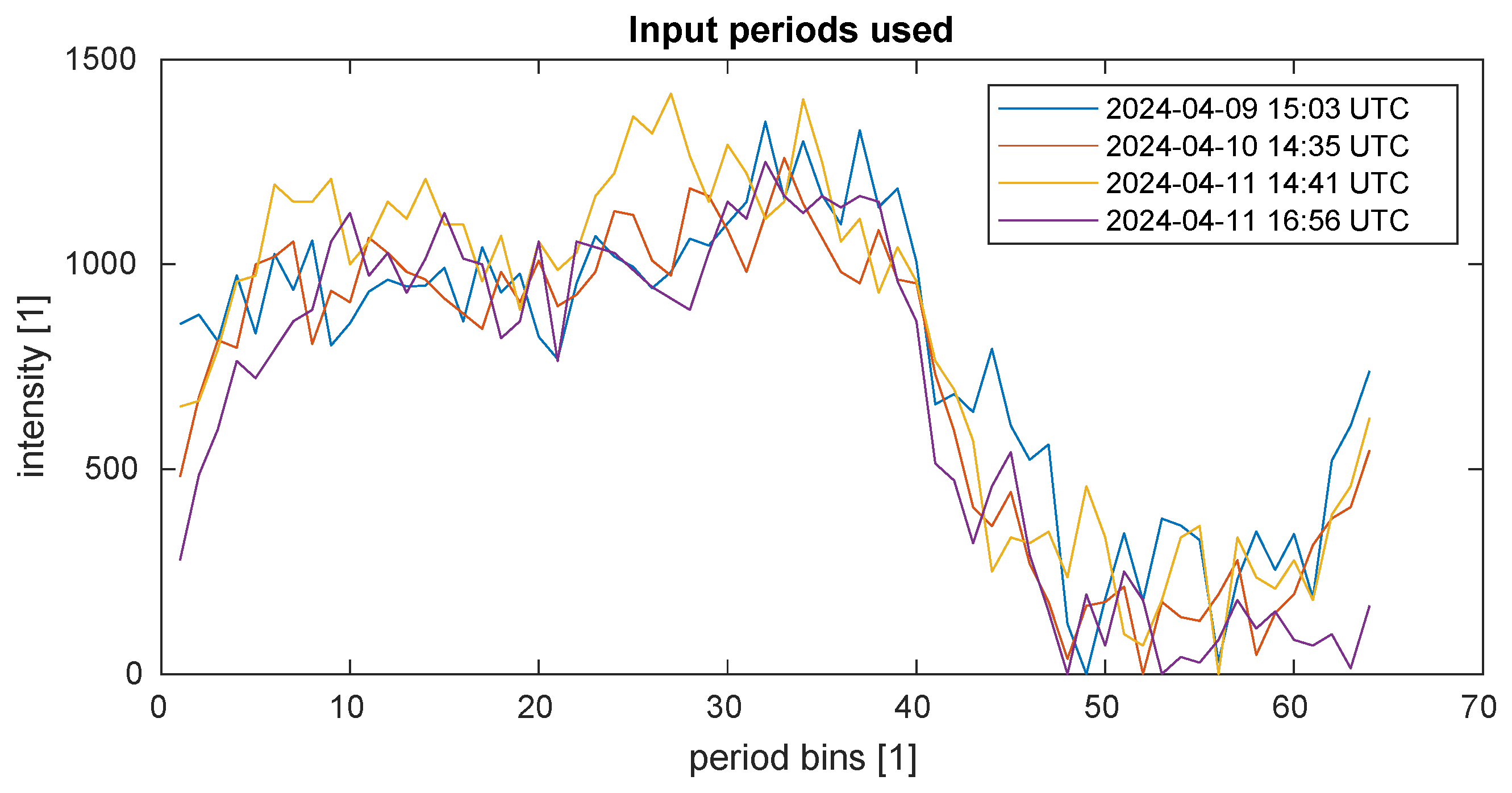
The required amount of additional noise will be added later when generating the output signal from the model. The next step is to remove the phase information from the model and keep it separate. Let us shift the first pulse profile so that the maximum of the pulse is in the bin center at $N_1/2$. The amount of rotation (number of bins) is converted to this profile’s initial phase ${\varphi }_{01}$. For all other pulses ($1<i\le M$), we use the cross-correlation of several periods of pulses to find a relative position with the highest match, and the required rotation of such pulse is its initial phase ${\varphi }_{0i}$. Aligned and processed input period shape examples for four observations of PSR B0950+08 can be seen in Figure 8.

The resulting cross-section of the model is then used for a single-pulse period shape. For this, the start and end of the pulse shape should have the same value to avoid steps in the resulting periodic signal. To achieve this, the model will use two pulse periods with half the period added before and half after the original period shape. Only the central part with a single-pulse profile is utilized to generate output from the cross-section of the model. These double-pulse profile shapes create one plane of the resulting model. The third axis is the time of the observation.

For the GPR-based model, the proper mean and kernel functions need to be selected. For simple shapes of pulses, single SEK was selected as a kernel function. The RQK can be utilized to model more trends in input data at once but at the expense of an additional hyperparameter. For binary pulsars where periodic behavior with a known frequency is expected, using the ESSK should be considered. The selection of the right kernel is carried out based on known physical properties of a given pulsar signal and tested by comparing the marginal likelihood of GPR models for each kernel candidate. For PSR B0950+08, as an example, a zero mean function and a single SEK kernel function with the following hyperparameters were used: a characteristic length scale of $3.67$, a signal standard deviation of $528.48$ and a noise standard deviation of $7.39$. Other kernels provided similar marginal likelihoods, as summarized in

Table 3. Marginal likelihood for different GPR kernels and PSR B0950+08 model.

Kernel	Marginal Likelihood [1]
SEK	$0.3242\times {10}^4$
Matérn kernel	$0.3258\times {10}^4$
RQK	$0.3354\times {10}^4$

, meaning there is no advantage in the selection of more computationally expansive kernels. ESSK was not tested as the parameter evolution is not periodic for PSR B0950+08.

3.2.2. Model-Based Signal Generator

Using the previously described model, artificial data can be generated for a randomly chosen time in the range of $T_1$ to $T_M$. The proper pulse period, phase, and shape for a given time $T_g\in [T_1,T_M]$ will be required to generate the signal. The generator output will be a discrete event list with selected time granularity. For examples in this section, the time increment of 1 $\mathrm{m}$$\mathrm{s}$ was used.

For the pulse period, the authors used the list of periods $\left\{P_i\right\}$ for observation start times $\left\{T_{0i}\right\}$ and constructed a cubic spline interpolation to evaluate period $P_g$ for time $T_g$. The GPR-based model and its cross-section in time $T_g$ is used for pulse shape. To obtain the initial phase ${\varphi }_g$ at time $T_g$, we chose the time $T_{0s}$ from $\left\{T_{0i}\right\}$ with minimal distance to $T_g$ and applied the Equation (7) using numeric integration to obtain phase ${\varphi }_g$ for $T_g$. Phase $\varphi \in [0,2\pi ]$ of a periodic signal in time $T_g$ depends on changing period P and initial phase ${\varphi }_{0s}$ [76]:

$${\varphi }_g=\varphi \left(T_g\right)={\int }_{T_{0s}}^{T_g}\omega \left(t^{\prime }\right)d{t}^{\prime }+{\varphi }_{0s}={\int }_{T_{0s}}^{T_g}{\displaystyle \frac{2\pi }{P\left(t^{\prime }\right)}}d{t}^{\prime }+{\varphi }_{0s}$$

(7)

Resulting profile for $T_g$ with initial phase ${\varphi }_g$ can be seen in Figure 9. The orange part of the profile is the single period used for further signal generation.

In current synthetic pulsar signal generators [55], the pulse profile model is based on very high SNR data from large telescopes like Effelsberg [77]. In our case, a smaller radio telescope was used, resulting in a lower SNR of obtained pulse even with several hours of single-pulsar observation. This means that the signal noise is a genuine part of our model and is only partially removed using minimum signal subtraction.

In previous works [44,78], it was shown that individual photon arrival at the detector can be seen as a cyclostationary non-homogeneous Poisson process. While several advanced pulsar generator methods were developed [55,56,79], these do not focus on the characteristic of the resulting signal but only on the generator’s efficiency to allow for a high-speed synthetic pulsar signal output. In this work, this is not the goal, so the authors utilized the direct method from Section 1.4, which can be replaced with a more advanced version if the throughput is of fundamental importance.

For the given time $T_g$ and selected time precision of 1 $\mathrm{m}$$\mathrm{s}$ in all examples shown, the probability of detecting k photons in the output bin is given by the Poisson distribution with parameter $\Lambda =I^{\prime }/s$, where $I^{\prime }$ is the profile intensity from a GPR-based model for a given bin, and s is the scaling factor for the amount of additional noise added to the pulsar signal.

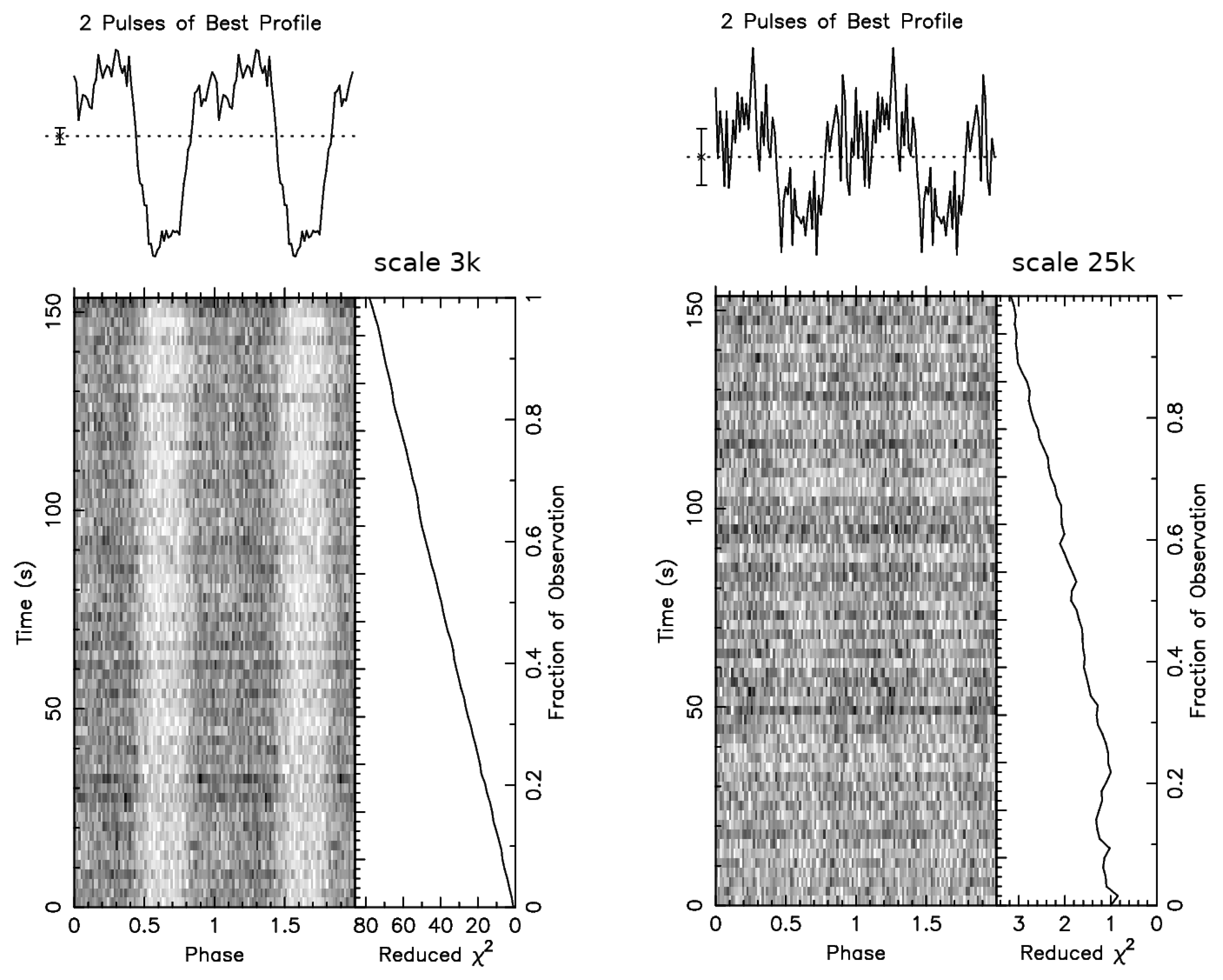
To illustrate the influence of scaling factor s, Figure 10 shows the results of processing 200 $\mathrm{s}$ of signal generated from the PSR B0950+08 GPR model for the same time $T_g$ but with a different scale s ranging from 3000, meaning a very small amount of noise added, to 25,000, meaning a high amount of noise added. The baseline-added background noise is the same for both cases. The possible minimal value for the scale $s=1$ means the exact model match for $\Lambda$. The maximal value is unlimited, but above some threshold, the pulsar signal is not detectable for a given signal length. For the model used in Figure 10, the threshold for s is $s_{thr}\approx \mathrm{40,000}$. In the same way, the background and measurement noise can be added and tuned. Examples in Figure 10 use uniform distribution $U(0,1)$.

3.3. Pulse Detection Statistics

In Section III b and Appendix B of [80], the use of reduced ${\chi }^2$ statistics for the determination of pulsation presence is discussed. The statistic S is defined as

$$S=\sum _{j=1}^n{\displaystyle \frac{{(R_j-\frac{N}{T^{\prime }})}^2}{\frac{N{T}_j}{T^{\prime }}}}$$

(8)

where n is the number of bins, N is the total number of photons received, $T_j$ is the total integration time for bin j, $T^{\prime }$ is the total integration time, and $R_j$ is the counting rate in bin j. It is proven that S is a ${\chi }_{n-1}^2$ random variable. To be independent of the number of bins, a reduced ${\chi }^2$ is often used, as defined by ${\chi }_r^2=S/(n-1)$. The local increase in ${\chi }_r^2$ for a given period P, its derivatives, and $DM$ are characteristic for pulsating signals processed with epoch folding. ${\chi }_r^2$ is one of the metrics used in PRESTO, HEASARC, and other pulsar-related software to evaluate the candidate parameters for the given signal with respect to pulsar signal detection [81,82]. The uncommon utilization of ${\chi }^2$ statistics use is explained in Section 4.3 of [83]. An example of ${\chi }_r^2$ dependency on period and its first derivative for the PSR B0818-13 signal can be seen in Figure 11.

This statistics-based comparison can be utilized instead of a direct pulse and timing comparison for calibration of a generated signal and NICER-recorded signal to obtain proper noise parameters for the generator.

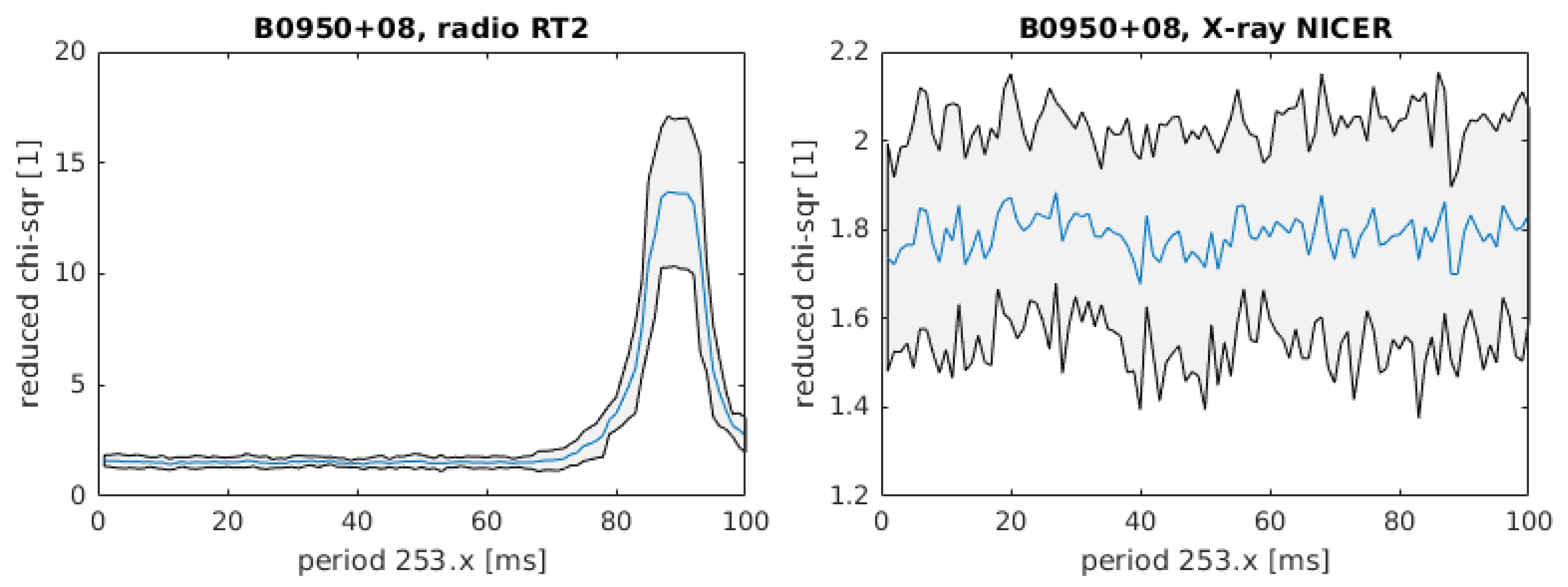
Figure 12 shows the mean value of reduced ${\chi }^2$ (blue line) and $1\sigma$ (gray area) of PSR B0950+08 for 4 observations of the radio signal from the RT2 telescope (left) and for 13 available observations of the X-ray signal from NICER (right). For signals with detectable pulses (long observation, high SNR), there is a significant peak in reduced ${\chi }^2$ values. The position of the peak is centered around the period of pulsar observed and thus is the same for all observations, while the amplitude of the peak depends on the quality of pulse detection.

The pulse period of $253.88$ $\mathrm{m}$$\mathrm{s}$ was detected for radio data, but there is no peak for the NICER data. The local peak around the expected $253.07$ $\mathrm{m}$$\mathrm{s}$ period is not higher than other local peaks caused purely by noise.

To demonstrate the behavior of reduced ${\chi }^2$ statistics with a changing SNR, driven by the generator parameter scale s and length of processed signal l, see Figure 13 for 600 $\mathrm{s}$ and 1200 $\mathrm{s}$ of generated signal. The background noise for these two examples was generated using uniform distribution $U(0,50)$. Each colored line in these graphs represents a different scale s for the generated signal.

Note that the longer the signal used, the higher the reduced ${\chi }^2$ value, but also, the width of the peak for the correct period is narrower. The shape of the peak is similar for different scales if the SNR is high enough to detect the pulse. If the pulse is not detected, the peak is not present, and the mean value of reduced ${\chi }^2$ is constant for all tested period values (253.00 $\mathrm{m}$$\mathrm{s}$–253.99 $\mathrm{m}$$\mathrm{s}$). For scale $s=3000$, the duration $t=600 \mathrm{s}$ of the signal is not enough to detect the pulse, while with $t=1200 \mathrm{s}$, the peak is clearly visible.

Figure 14 and Figure 15 demonstrate the evolution of reduced ${\chi }^2$ statistics for different folding periods close to the target period with decreasing signal length l and decreasing amount of noise and increasing SNR via scale s.

3.4. Surrogate Pulsar Signal Model Validation

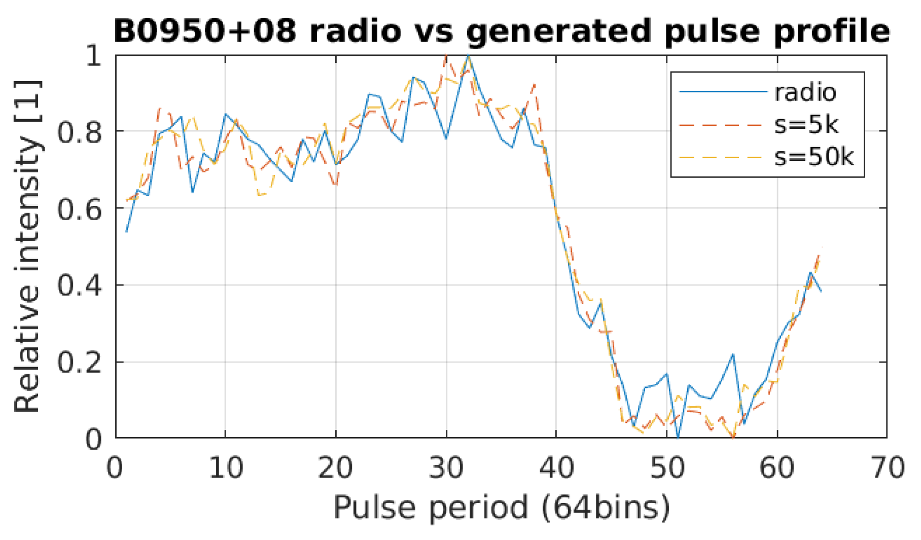
For generated data, the output needs to be validated with respect to the original measured data. To compare differences between the original radio-based pulse profile and two generated data-based pulse profiles with high and low SNR, see Figure 16.

The standard mean for comparing two curves or sets of samples is the coefficient of determination, defined as the squared Pearson correlation coefficient. To validate the generated pulsar data, they are first processed with PRESTO to obtain an integrated pulse profile and period. These are then compared to values derived from measured data processed with PRESTO using the coefficient of determination $R^2$, where $R^2=r_{xy}^2$. The Pearson correlation coefficient $r_{xy}$ for N samples of original x and generated y pulsar profiles is then defined as [58]:

$$r_{xy}={\displaystyle \frac{{\sum }_{i=1}^N(x_i-{\overline{x}}_i)(y_i-{\overline{y}}_i)}{\sqrt{{\sum }_{i=1}^N{(x_i-{\overline{x}}_i)}^2}\sqrt{{\sum }_{i=1}^N{(y_i-{\overline{y}}_i)}^2}}}$$

(9)

with $\overline{x}$ being the mean value of x and $\overline{y}$ being the mean value of y.

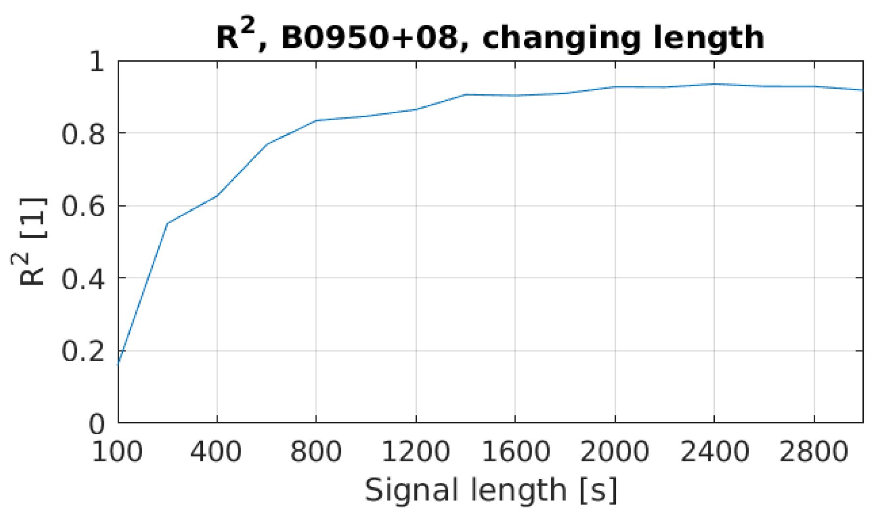
The original measured data and generated data with changing parameters are compared, and a change in SNR via scale s and length of generated signal l is evaluated. The generated signal is compared to the closest radio observation data in the time domain, so the $R^2$ coefficient never reaches $1.0$; there is an approximation of the original pulse profile within GPR training and the model pulse profile for time $T_g$ is different than the pulse profile for time $T_{0i}$ if $|T_{0i}-T_g|>0$. These evaluations provide inputs for proper sensor and observation length selection for simulations or HIL testing.

Figure 17 shows the evolution of $R^2$ with the changing scale of s within the generator and constant length of signal $l=3000$ [s]. With the scale below ∼25,000, the $R^2$ is within the $10\%$ margin of its maximum, which corresponds with the signal processing output from PRESTO. With a lower SNR caused by a higher scale of s, the $R^2$ decreases.

Figure 18 shows the evolution of $R^2$ when changing the length of the generated signal l and the constant scale $s=$ 25,000.

The last thing to test is the stability of $R^2$ with a signal of constant scale s and length l but generated for different times $T_g$. Figure 19 shows the evolution of $R^2$ for scale $s=$ 25,000 and signal length $l=3000$ [s] with the signal generated to start on 2024-04-10 x:00:00.0 with $x\in {\mathbb{N}}_0,0\le x\le 23$. In contrast to previous tests, where just the resulting pulse profiles without any change can be compared, here there are different pulse phases $\Phi$ for every generated signal. To compare them with the original radio-based pulse profile, these generated profiles need to be shifted to have the same phase $\Phi$. The resulting evolution of $R^2$ within one day of the generated signal is stable as expected, with small fluctuations due to randomness in the signal generator.

4. Discussion

To the authors’ best knowledge, all other existing methods for synthetic pulsar signal generation focus on the computational complexity of the process to allow for the maximal amount of generated signal per computational time.

What all these methods have in common is the original source of pulsar characteristics. They work with the exact pulse period, in some cases complemented by its first- or even second-time derivative, and the best available pulse profile shape obtained from independent projects utilizing the best available space or Earth-based observatories. This leads to the limitation of pulsar selection, amount of observation per pulsar, and dependency on third-party projects. The evolution of pulsar signal characteristics, as well as background noise, is not taken into consideration.

The newly proposed method for pulsar signal modeling is based on the utilization of radio observation from a smaller Earth-based radio telescope, balancing the data quality with a higher availability of this class telescopes. This results in a much higher number of possible observations. These observations are used as input for the pulsar signal model with all parameters set as flexible instead of fixed. This allows for not only a generic pulse period evolution in time but also profile shape change. Such a model is closer to conditions that the sensor will work with for real applications and thus provides higher confidence for XNAV simulations or HIL tests for future sensor development. As the model defines the pulsar signal characteristics only, it serves as input data replacement for all previously mentioned methods and, as such, can improve the results of all of them.

Future Trends

The authors expect to participate in further improvements in the current demonstration setup of the RT2 radio telescope to enable automatic observation planning and real-time radio signal processing. With these enhancements, it will be possible to build a whole stack of necessary processing blocks for the implementation of a pulsar clock. The authors will make the database of recorded pulsar signals publicly available for further scientific use. Once the RT2 system is thoroughly tested and developed, it is expected to apply the setup for the available 11 $\mathrm{m}$ RT5 radio telescope. This should enable us to extend the list of pulsars with detectable signals and find a better overlap with NICER X-ray data for further calibration and extension of the current pulsar signal model.

References

1. Anderson, K.; Pines, D.; Sheikh, S. Validation of Pulsar Phase Tracking for Spacecraft Navigation. J. Guid. Control Dyn. 2015, 38, 1–13. [Google Scholar] [CrossRef]
2. Graven, P.; Collins, J.; Sheikh, S.; Hanson, J.; Ray, P.; Wood, K. XNAV for deep space navigation. In Proceedings of the 31st Annual AAS Guidance and Control Conference, Breckenridge, CO, USA, 1–6 February 2008. [Google Scholar]
3. Sheikh, S. The Use of Variable Celestial X-ray Sources for Spacecraft Navigation. Ph.D. Thesis, University of Maryland, College Park, MD, USA, 2005. [Google Scholar]
4. Smith, R.; Sheikh, S.; Swinney, R. Navigation to the Alpha Centauri star system. J. Br. Interplanet. Soc. 2017, 69, 379–389. [Google Scholar]
5. Lorimer, D.R. Binary and Millisecond Pulsars. Living Rev. Relativ. 2005, 8, 7. [Google Scholar] [CrossRef] [PubMed]
6. Lynch, R.S. Pulsar Timing Arrays. J. Phys. Conf. Ser. 2015, 610, 012017. [Google Scholar] [CrossRef]
7. Dyks, J. Geometry of radio pulsar signals: The origin of pulsation modes and nulling. Astron. Astrophys. 2021, 653, L3. [Google Scholar] [CrossRef]
8. Lorimer, D.R.; Kramer, M. Handbook of Pulsar Astronomy; Cambridge University Press: Cambridge, UK, 2012. [Google Scholar]
9. Lyne, A.; Graham-Smith, F. Pulsar Astronomy, 4th ed.; Cambridge Astrophysics, Cambridge University Press: Cambridge, UK, 2022. [Google Scholar]
10. Pennucci, T.T.; Possenti, A.; Esposito, P.; Rea, N.; Haggard, D.; Baganoff, F.K.; Burgay, M.; Zelati, F.C.; Israel, G.L.; Minter, A. Simultaneous Multi-band Radio and X-ray Observations of the Galactic Center Magnetar SGR 1745–2900. Astrophys. J. 2015, 808, 81. [Google Scholar] [CrossRef]
11. Koziel, S.; Leifsson, L. Introduction to Surrogate Modeling and Surrogate-Based Optimization; Springer: Cham, Switzerland, 2016; pp. 31–61. [Google Scholar] [CrossRef]
12. Cristianini, N.; Shawe-Taylor, J. An Introduction to Support Vector Machines and Other Kernel-Based Learning Methods; Cambridge University Press: Cambridge, UK, 2001. [Google Scholar] [CrossRef]
13. Duvenaud, D. Automatic Model Construction with Gaussian Processes. Ph.D. Thesis, Cambridge University Press, Cambridge, UK, 2014. [Google Scholar] [CrossRef]
14. Roberts, S.J.; Osborne, M.A.; Ebden, M.; Reece, S.; Gibson, N.P.; Aigrain, S. Gaussian processes for time-series modelling. Philos. Trans. R. Soc. A Math. Phys. Eng. Sci. 2013, 371, 20110550. [Google Scholar] [CrossRef]
15. de Visser, C. Global Nonlinear Model Identification with Multivariate Splines. Ph.D. Thesis, Delft University of Technology, Delft, The Netherlands, 2011. [Google Scholar]
16. Rasmussen, C.E.; Williams, C.K.I. Gaussian Processes for Machine Learning; The MIT Press: Cambridge, MA, USA, 2005. [Google Scholar] [CrossRef]
17. Queipo, N.V.; Haftka, R.T.; Shyy, W.; Goel, T.; Vaidyanathan, R.; Kevin Tucker, P. Surrogate-based analysis and optimization. Prog. Aerosp. Sci. 2005, 41, 1–28. [Google Scholar] [CrossRef]
18. Schreiber, T.; Schmitz, A. Surrogate time series. Phys. D Nonlinear Phenom. 2000, 142, 346–382. [Google Scholar] [CrossRef]
19. Wang, Y.; Wang, Y.; Zheng, W. A Gaussian Process Surrogate Model Assisted Multi-optimization Algorithm for Pulsar Period Searching. In Proceedings of the China Satellite Navigation Conference (CSNC 2024) Proceedings, Jinan, China, 22–24 May 2024; Yang, C., Xie, J., Eds.; Springer Nature: Singapore, 2024; pp. 320–330. [Google Scholar]
20. Batrakov, A.; Hu, H.; Wex, N.; Freire, P.; Venkatraman Krishnan, V.; Kramer, M.; Guo, Y.; Guillemot, L.; McKee, J.; Cognard, I.; et al. A new pulsar timing model for scalar-tensor gravity with applications to PSR J2222-0137 and pulsar-black hole binaries. Astron. Astrophys. 2023, 686, A101. [Google Scholar] [CrossRef]
21. Kedia, A.; Ristic, M.; O’Shaughnessy, R.; Yelikar, A.B.; Wollaeger, R.T.; Korobkin, O.; Chase, E.A.; Fryer, C.L.; Fontes, C.J. Surrogate light curve models for kilonovae with comprehensive wind ejecta outflows and parameter estimation for AT2017gfo. Phys. Rev. Res. 2023, 5, 013168. [Google Scholar] [CrossRef]
22. Alizadeh, R.; Allen, J.K.; Mistree, F. Managing computational complexity using surrogate models: A critical review. Res. Eng. Des. 2020, 31, 275–298. [Google Scholar] [CrossRef]
23. Ben Salem, M.; Tomaso, L. Automatic selection for general surrogate models. Struct. Multidiscip. Optim. 2018, 58, 719–734. [Google Scholar] [CrossRef]
24. Garud, S.S.; Karimi, I.; Kraft, M. Smart Sampling Algorithm for Surrogate Model Development. Comput. Chem. Eng. 2017, 96, 103–114. [Google Scholar] [CrossRef]
25. Huang, T.; Liu, Y.; Pan, Z. Deep Residual Surrogate Model. Inf. Sci. 2022, 605, 86–98. [Google Scholar] [CrossRef]
26. Xu, Y.; Renteria, A.; Wang, P. Adaptive surrogate models with partially observed information. Reliab. Eng. Syst. Saf. 2022, 225, 108566. [Google Scholar] [CrossRef]
27. Zhang, J.; Chowdhury, S.; Messac, A. An adaptive hybrid surrogate model. Struct. Multidiscip. Optim. 2012, 46, 223–238. [Google Scholar] [CrossRef]
28. Kocijan, J. Modelling and Control of Dynamic Systems Using Gaussian Process Models; Springer: Cham, Switzerland, 2016. [Google Scholar] [CrossRef]
29. Wang, J. An Intuitive Tutorial to Gaussian Process Regression. Comput. Sci. Eng. 2023, 25, 4–11. [Google Scholar] [CrossRef]
30. Williams, B.; Cremaschi, S. Selection of surrogate modeling techniques for surface approximation and surrogate-based optimization. Chem. Eng. Res. Des. 2021, 170, 76–89. [Google Scholar] [CrossRef]
31. Gutmann, H.M. A Radial Basis Function Method for Global Optimization. J. Glob. Optim. 2001, 19, 201–227. [Google Scholar] [CrossRef]
32. Lawrence, N.; Seeger, M.; Herbrich, R. Fast Sparse Gaussian Process Methods: The Informative Vector Machine. Adv. Neural Inf. Process. Syst. 2002, 15, 625–632. [Google Scholar]
33. Wang, Y.; Zheng, W.; Zhang, S.; Ge, M.; Li, L.; Jiang, K.; Chen, X.; Zhang, X.; Zheng, S.; Lu, F. Review of X-ray pulsar spacecraft autonomous navigation. Chin. J. Aeronaut. 2023, 36, 44–63. [Google Scholar] [CrossRef]
34. Han, W.; Wang, N.; Wang, J.; Yuan, J.; He, D. Using single millisecond pulsar for terrestrial position determination. Astrophys. Space Sci. 2019, 364, 48. [Google Scholar] [CrossRef]
35. Buist, P.J.; Engelen, S.; Noroozi, A.; Sundaramoorthy, P.; Verhagen, S.; Verhoeven, C. Overview of Pulsar Navigation: Past, Present and Future Trends. Navigation 2011, 58, 153–164. [Google Scholar] [CrossRef]
36. Emadzadeh, A.A.; Speyer, J. Navigation in Space by X-ray Pulsars; Springer: Berlin/Heidelberg, Germany, 2011. [Google Scholar]
37. Shen, L.R.; Li, X.P.; Sun, H.F.; Fang, H.Y.; Xue, M.F. A novel period estimation method for X-ray pulsars based on frequency subdivision. Front. Inf. Technol. Electron. Eng. 2015, 16, 858–870. [Google Scholar] [CrossRef]
38. Liu, J.; Yang, Z.-H.; Kang, Z.-W.; Chen, X. Fast CS-based pulsar period estimation method without tentative epoch folding and its CRLB. Acta Astronaut. 2019, 160, 90–100. [Google Scholar] [CrossRef]
39. Cassanelli, T.; Naletto, G.; Codogno, G.; Barbieri, C.; Verroi, E.; Zampieri, L. New technique for determining a pulsar period: Waterfall principal component analysis. Astron. Astrophys. 2022, 663, A106. [Google Scholar] [CrossRef]
40. Ma, X.; Xie, T.; Li, J.; Zhang, W.; Cheng, Y.; Cui, P.; Ning, X. An energy-based pulsar period estimation method using Hilbert curve and double CNNs. Acta Astronaut. 2024, 219, 79–90. [Google Scholar] [CrossRef]
41. Xie, T.H.; Ma, X.; Zhang, W.J.; Li, J.R.; Wang, S.T.; Yang, Z.N.; Cui, P.L.; Ning, X.L.; Fang, J.C. Dynamic estimation method for pulsar periods based on photon energy distribution folding and image template matching. Astron. Astrophys. 2024, 686, A214. [Google Scholar] [CrossRef]
42. Wei, Z.; Yidi, W. X-ray Pulsar-Based Navigation: Theory and Applications; Springer: Berlin/Heidelberg, Germany, 2020. [Google Scholar]
43. Zhou, Q.; Liu, S.; Hao, X.; Jiang, K. A Relativistic Model of X-Ray Pulsar Signal for Navigation. In Proceedings of the China Satellite Navigation Conference (CSNC 2022) Proceedings, Beijing, China, 25–27 May 2022; Yang, C., Xie, J., Eds.; Springer Nature: Singapore, 2022; pp. 433–441. [Google Scholar]
44. Sala, J.; Urruela, A.; Villares, X.; Estalella, R.; Paredes, J.M. Feasibility Study for a Spacecraft Navigation System Relying on Pulsar Timing Information (Final Report); Adv Res Team of ESA 1-90. Technical Report; ESA Advanced Concepts Team: Noordwijk, The Netherlands, 2004. [Google Scholar]
45. Sheikh, S.I.; Hanson, J.E.; Collins, J.; Graven, P. Deep Space Navigation Augmentation Using Variable Celestial X-ray Sources. Proc. Inst. Navig. Natl. Tech. Meet. 2009, 1, 34–48. [Google Scholar]
46. Zhang, X.; Shuai, P.; Huang, L.; Chen, S.; Xu, L. Mission Overview and Initial Observation Results of the X-ray Pulsar Navigation-I Satellite. Int. J. Aerosp. Eng. 2017, 2017, 8561830. [Google Scholar] [CrossRef]
47. Mitchell, J.W.; Hassouneh, M.; Winternitz, L.; Valdez, J.; Price, S.; Semper, S.R.; Yu, W.H.; Arzoumanian, Z.; Ray, P.; Wood, K.S.; et al. SEXTANT—Station Explorer for X-ray Timing and Navigation Technology. In Proceedings of the AIAA Guidance, Navigation, and Control Conference, Kissimmee, FL, USA, 5–9 January 2015. [Google Scholar] [CrossRef]
48. NASA. Catalogs and astronomical archives of the HEASARC. Available online: https://heasarc.gsfc.nasa.gov/docs/archive.html (accessed on 6 October 2024).
49. Lohan, K.G.; Putnam, Z.R. Characterization of Candidate Solutions for X-Ray Pulsar Navigation. IEEE Trans. Aerosp. Electron. Syst. 2024, 60, 2749–2762. [Google Scholar] [CrossRef]
50. Shemar, S.; Fraser, G.; Heil, L.; Hindley, D.; Martindale, A.; Molyneux, P.; Pye, J.; Warwick, R. Towards practical autonomous deep-space navigation using X-ray pulsar timing. Exp. Astron. 2016, 42, 101–138. [Google Scholar] [CrossRef]
51. Ren, X.; Nie, G.; Li, L. An Improved Augmented Algorithm for Direction Error in XPNAV. Symmetry 2020, 12, 1059. [Google Scholar] [CrossRef]
52. Xu, Q.; Wang, H.-L.; Feng, L.; You, S.-H.; He, Y.-Y. A novel X-ray pulsar integrated navigation method for ballistic aircraft. Optik 2018, 175, 28–38. [Google Scholar] [CrossRef]
53. Fu, L.; Shuai, P.; Xue, M.; Sun, H.; Fang, H. The Research of X-Ray Pulsar Signals Simulation Method. In Proceedings of the China Satellite Navigation Conference (CSNC) 2015 Proceedings, Xi’an, China, 13–15 May 2015; Sun, J., Liu, J., Fan, S., Lu, X., Eds.; Springer: Berlin/Heidelberg, Germany, 2015; Volume III, pp. 635–647. [Google Scholar]
54. Emadzadeh, A.A.; Speyer, J.L. On Modeling and Pulse Phase Estimation of X-ray Pulsars. IEEE Trans. Signal Process. 2010, 58, 4484–4495. [Google Scholar] [CrossRef]
55. Zhang, H.; Xu, L.; Song, S.; Jiao, R. A fast method for X-ray pulsar signal simulation. Acta Astronaut. 2014, 98, 189–200. [Google Scholar] [CrossRef]
56. Jin, J.; Liu, Y.; Li, X.; Shen, Y.; Huang, L. A simulation method for X-ray pulsar signal based on Monte Carlo. In Proceedings of the 2016 IEEE International Conference on Mechatronics and Automation, Harbin, China, 7–10 August 2016; pp. 1937–1942. [Google Scholar] [CrossRef]
57. Huang, Z.; Zong, H.; Xie, Y.; Yu, D.; Xu, Q.; Lu, K. X-ray pulsar observation signals simulation method at the spacecraft in near-Earth space. Adv. Space Res. 2024, 73, 6241–6254. [Google Scholar] [CrossRef]
58. Su, J.; Fang, H.; Bao, W.; Sun, H.; Shen, L.; Zhao, L. Fast simulation of X-ray pulsar signals at a spacecraft. Acta Astronaut. 2020, 166, 93–103. [Google Scholar] [CrossRef]
59. Green, R.M. Spherical Astronomy; Cambridge University Press: Cambridge, UK, 1985; p. 546. [Google Scholar]
60. Bilous, A.V.; Kondratiev, V.I.; Kramer, M.; Keane, E.F.; Hessels, J.W.T.; Stappers, B.W.; Malofeev, V.M.; Sobey, C.; Breton, R.P.; Cooper, S.; et al. A LOFAR census of non-recycled pulsars: Average profiles, dispersion measures, flux densities, and spectra. Astron. Astrophys. 2016, 591, A134. [Google Scholar] [CrossRef]
61. Jankowski, F.; van Straten, W.; Keane, E.F.; Bailes, M.; Barr, E.D.; Johnston, S.; Kerr, M. Spectral properties of 441 radio pulsars. Mon. Not. R. Astron. Soc. 2018, 473, 4436–4458. [Google Scholar] [CrossRef]
62. Kijak, J.; Basu, R.; Lewandowski, W.; Rożko, K.; Dembska, M. Gigahertz-peaked Spectra Pulsars and Thermal Absorption Model. Astrophys. J. 2017, 840, 108. [Google Scholar] [CrossRef]
63. Kijak, J.; Lewandowski, W.; Maron, O.; Gupta, Y.; Jessner, A. Pulsars with gigahertz-peaked spectra. Astron. Astrophys. 2011, 531, A16. [Google Scholar] [CrossRef]
64. Rożko, K.; Basu, R.; Kijak, J.; Lewandowski, W. The uGMRT Observations of Three New Gigahertz-peaked Spectra Pulsars. Astrophys. J. 2021, 922, 125. [Google Scholar] [CrossRef]
65. Armstrong, J.W.; Rickett, B.J.; Spangler, S.R. Electron Density Power Spectrum in the Local Interstellar Medium. Astrophys. J. 1995, 443, 209. [Google Scholar] [CrossRef]
66. Bhat, N.; Rao, A.; Gupta, Y. Long-Term Scintillation Studies of Pulsars: I. Observations and Basic Results. Astrophys. J. Suppl. 1999, 121, 483. [Google Scholar] [CrossRef]
67. Stinebring, D.R.; Smirnova, T.V.; Hankins, T.H.; Hovis, J.S.; Kaspi, V.M.; Kempner, J.C.; Myers, E.; Nice, D.J. Five Years of Pulsar Flux Density Monitoring: Refractive Scintillation and the Interstellar Medium. Astrophys. J. 2000, 539, 300. [Google Scholar] [CrossRef]
68. Puricer, P.; Kovář, P.; Barta, M. Modernized Solar Radio Spectrograph in the L Band Based on Software Defined Radio. Electronics 2019, 8, 861. [Google Scholar] [CrossRef]
69. Bates, S.D.; Lorimer, D.R.; Verbiest, J.P.W. The pulsar spectral index distribution. Mon. Not. R. Astron. Soc. 2013, 431, 1352–1358. [Google Scholar] [CrossRef]
70. Cameron, A.D.; Li, D.; Hobbs, G.; Zhang, L.; Miao, C.C.; Wang, J.B.; Yuan, M.; Wang, S.; Jacobs Corban, G.; Cruces, M.; et al. An in-depth investigation of 11 pulsars discovered by FAST. Mon. Not. R. Astron. Soc. 2020, 495, 3515–3530. [Google Scholar] [CrossRef]
71. Lorimer, D. SIGPROC: Pulsar Signal Processing Programs; Astrophysics Source Code Library, record ascl:1107.016; Michigan Technological University: Houghton, MI, USA, 2011. [Google Scholar]
72. Ransom, S. PRESTO: PulsaR Exploration and Search TOolkit; Astrophysics Source Code Library, record ascl:1107.017; Michigan Technological University: Houghton, MI, USA, 2011. [Google Scholar]
73. Gügercinoğlu, E.; Köksal, E.; Güver, T. On the peculiar rotational evolution of PSR B0950+08. Mon. Not. R. Astron. Soc. 2022, 518, 5734–5740. [Google Scholar] [CrossRef]
74. Taylor, J.H.; Manchester, R.N.; Lyne, A.G. Catalog of 558 Pulsars. Astrophys. J. Suppl. 1993, 88, 529. [Google Scholar] [CrossRef]
75. Wang, Z.; Lu, J.; Jiang, J.; Lin, J.; Lee, K.; Liang, E.; Xu, R. The radio signal of PSR B0950+08 is detected over the whole pulse phase. Mon. Not. R. Astron. Soc. 2022, 517, 5560–5568. [Google Scholar] [CrossRef]
76. Gregory, R.D. Classical Mechanics; Cambridge University Press: Cambridge, UK, 2006. [Google Scholar] [CrossRef]
77. Kramer, M. Geometrical analysis of average pulsar profiles using multi-component Gaussian FITS at several frequencies. II. Individual results. Astron. Astrophys. Suppl. 1994, 107, 527–539. [Google Scholar]
78. Zhang, H.; Xu, L.P.; Xie, Q.; Luo, N. X-ray pulsar weak signal detection based on Bayesian estimation. Wuli Xuebao/Acta Phys. Sin. 2011, 60. [Google Scholar] [CrossRef]
79. Hazboun, J.; Shapiro-Albert, B.; Baker, P.; Henkel, A.; Wagner, C.; Hesse, J.; Brook, P.; Lam, M.; McLaughlin, M.; Garver-Daniels, N. The Pulsar Signal Simulator: A Python package for simulating radio signal data from pulsars. J. Open Source Softw. 2021, 6, 2757. [Google Scholar] [CrossRef]
80. Leahy, D.A.; Darbro, W.; Elsner, R.F.; Weisskopf, M.C.; Sutherland, P.G.; Kahn, S.; Grindlay, J.E. On searches for pulsed emission with application to four globular cluster X-ray sources: NGC 1851, 6441, 6624 and 6712. Astrophys. J. 1983, 266, 160–170. [Google Scholar] [CrossRef]
81. Fang, H.; Sun, X.; Yao, Y.; Li, L.; Su, J.; Zhang, L. Analysis on numerical mutation in cost function of Chi-square test for frequency search of Crab pulsar. Digit. Signal Process. 2022, 129, 103688. [Google Scholar] [CrossRef]
82. Xu, N.; Sheng, L.; Chen, C.; Li, Y.; Su, T.; Zhao, B.; Zheng, W.; Liu, C. Application of Gaussian fitting to the fast search of pulsar periodic. Optik 2019, 198, 163253. [Google Scholar] [CrossRef]
83. Lynch, R. Searching for and Identifying Pulsars; Technical report; Department of Astronomy, University of Virginia: Charlottesville, VA, USA, 2008. [Google Scholar]
Figure 1. Pulsar signal time evolution—current models (a) and proposed model (b) considering ISM instabilities and reduced on-board sensor sensitivity.
Aerospace 11 00839 g001
Figure 2. Pulsar navigation system architecture. Source: [34].
Aerospace 11 00839 g002
Figure 3. Highest flux pulsars and their estimation. The gray area on the map is never visible when using the RT2 radio telescope.
Aerospace 11 00839 g003
Figure 4. The RT2 radio telescope in CAS Ondřejov observatory.
Aerospace 11 00839 g004
Figure 5. Pulsar signal model with time evolution—current models (a) and proposed model (b).
Aerospace 11 00839 g005
Figure 6. GPR-based pulsar signal surrogate model utilization in the whole signal generator pipeline.
Aerospace 11 00839 g006
Figure 7. GPR-based pulsar radio signal model for PSR B0950+08.
Aerospace 11 00839 g007
Figure 8. Input period shapes after normalization, minimum subtraction, and phase removal for PSR B0950+08.
Aerospace 11 00839 g008
Figure 9. PSR B0950+08 pulse profile for selected time T g with initial signal-phase ϕ g (vertical black line). The orange part of the profile is a single period used for signal generation.
Aerospace 11 00839 g009
Figure 10. Generated signals of PSR B0950+08 processed with PRESTO for different scales of s (SNR).
Aerospace 11 00839 g010
Figure 11. Reduced χ 2 statistic versus period and its first derivative for PSR B0818-13 (1239 ms).
Aerospace 11 00839 g011
Figure 12. Reduced χ 2 statistics for PSR B0950+08—radio vs. X-ray ( 253.88 m s ).
Aerospace 11 00839 g012
Figure 13. Reduced χ 2 statistic for 600 s and 1200 s of generated PSR B0950+08 signal (253.88 ms).
Aerospace 11 00839 g013
Figure 14. Evolution of reduced χ 2 statistic shape for length of signal l decreasing left to right.
Aerospace 11 00839 g014
Figure 15. Evolution of reduced χ 2 statistic shape for scale s decreasing from left to right.
Aerospace 11 00839 g015
Figure 16. Pulse profiles based on measured (blue) and generated data with high SNR (red) and low SNR (yellow) for PSR B0950+08.
Aerospace 11 00839 g016
Figure 17. Coefficient of determination for the PSR B0950+08 changing scale s.
Aerospace 11 00839 g017
Figure 18. Coefficient of determination for the PSR B0950+08 changing length l.
Aerospace 11 00839 g018
Figure 19. Coefficient of determination for the PSR B0950+08 changing time T g during 2024-04-10.
Aerospace 11 00839 g019