Rapid Evaluation of the Destructive Power Caused by Accidental Explosion of Space Launch Vehicles

Abstract

Space launch vehicles are usually loaded with a large amount of propellant, and the destructive power caused by their explosion is significant. The altitude of an accidental explosion will lead to differences in the destructive power, because the environmental parameters of different altitudes are different, and the explosion shock wave parameters are closely related to the environmental parameters. Therefore, it was necessary to establish a set of analytical methods to rapidly analyze the relationship between altitude and the explosion shock wave parameters. A large number of simulation conditions were tested at 0~10 km altitude using the nonlinear dynamics software AUTODYN. The relationship between the explosion shock wave pressure P, the proportional distance z, and the altitude h was obtained, which could be used to rapidly characterize the explosion shock wave pressures at different altitudes. A comparative analysis was conducted with the experimental results to verify the scientificity of the fitting formula. The results indicate that the error between the experimental and calculated values is less than 5.80%, indicating that the rapid evaluation formula established in this paper is reasonable. These findings not only enrich the theory related to explosion shock waves, but also provide a rapid analysis basis for the accidental explosion of space launch vehicles.

1. Introduction

With the rapid development of science and technology, human exploration of space has progressed from the initial exploration of near-Earth space to the current exploration of deep space. In the process of exploring the universe, a variety of space launch vehicles have been developed, such as airships, airplanes, space shuttles, rockets, starships, and so on. The above space launch vehicles are simply huge fuel storage tanks containing a large amount of liquid or solid fuel. If there are problems with the launch process, causing the vehicle to explode, the destructive power can be massive. In the history of international space launches, many famous air disasters and accidents have occurred [1]. Among them, the launch accidents of the NASA space shuttle Challenger on 28 January 1986 and the NASA space shuttle Columbia on 1 February 2003 were particularly serious, both resulting in the deaths of all astronauts aboard [2,3]. The most recent launch accident was the Starship SN11 launched by SpaceX on 20 April 2023, which exploded about 2 min after liftoff and was loaded with over 4500 metric tons of propellant [4]. The explosion of a space launch vehicle produces a huge explosion shock wave, which can be destructive to personnel, equipment, and facilities. On 3 July 1969, a Soviet N1 rocket fell back onto the launch pad shortly after launch and caused a violent explosion. The power of this explosion exceeded 1000 tons of TNT explosives, almost completely destroyed the launch site, and produced a blaze that could be seen nearly 40 km away. On 15 February 1996, the CZ-3B rocket was launched from Xichang Satellite Launch Center and crashed into a mountain after careening out of control. The blast wave and the volatilization of highly toxic fuel caused many casualties. In 2022, there were 186 space launches worldwide, far exceeding the 114 carried out in 2020 and the 145 in 2021, of which 178 were successful and 8 failed. Faced with such high frequency space launch activities, space launch safety has become increasingly important. Therefore, it was necessary to establish a set of methods to rapidly evaluate the destructive power of space launch vehicles after accidental explosions, whether from the perspective of launch site safety or post-accident analysis. The destructive power of space vehicles during ground explosions and high-altitude explosions is different, as there are significant differences between the atmospheric environmental parameters at high altitudes and those on the ground. Based on the above considerations, this paper conducted an analysis of the destructive power of space launch vehicles after accidental explosions at different atmospheric environments. In order to facilitate the analysis, the fuel loaded on space vehicles was uniformly equivalent to the corresponding equivalent TNT explosive for this research.

In engineering applications, there have been many engineering examples [5,6] that were required to take into account the influence of the external environment on the propagation characteristics of explosion shock waves. If parameters such as air density, oxygen content, and wave velocity change, it can cause significant differences in the destructive power field. The explosion effect parameters used in standard specifications are mostly based on ambient temperature in low altitude areas. If they are not modified in high-altitude areas, large errors can occur. The parameters of the near-field characteristics of air explosions include the peak overpressure ΔP, the specific impulse i, the positive pressure action time t+, the shock wave arrival time t′, etc. In order to calculate these parameters, researchers have put forward their own calculation formulas, obtained through a large number of experiments. The early commonly used experience formulas mainly included Henrych’s formula [7], Sadovskyi’s formula [8], Brode’s formula [9], Aliansov’s formula [10], Baker’s formula [11], etc. These empirical formulas have different application scopes, and there are differences between them. In 1887, Rankine and Hugoniot established the equation of state of a shock wave, clearly pointing out that the adiabatic reversible transition of a shock wave violates the principle of energy conservation, thus laying the foundation for the theoretical study of shock waves [12]. Cullis elaborated the mechanism of the formation of explosion shock waves in detail, and systematically elaborated the basic principle of the interaction between explosion shock waves and complex structures [13]. Goodman [14] processed free field explosion wave data, compiled the peak overpressure, specific impulse, and positive pressure action time of spherical explosive tests from 1945 to 1960, and created the fitting curve of the incident overpressure peak and specific impulse experimental data. When the external air environment (such as pressure, temperature, etc.) changes, the law of the above characteristic parameters will change accordingly [15]; that is, the Sachs’s proportional law will be satisfied [16]. Ericsson [17] and Glasstone [18] conducted a series of explosion experiments to test the validity of Sachs’s proportional law. Jack [19] found that the properties of an explosion shock wave will change under the above conditions when carrying out simulated high-altitude explosion tests, and the Sachs’s proportional law cannot be used for the conversion of characteristic parameters at this time. Therefore, many researchers have considered the propagation law of explosion shock waves under different pressure environments, obtaining valuable research results. Veldman [20] used a spherical sealed container with variable ambient pressure to carry out an explosion experiment on C-4 explosives, and studied the influence of ambient pressure on the overpressure and impulse of reflected shock waves. Silnikov [6] studied the relationship between the shock wave parameters of high explosives and the air pressure based on the similarity criterion of explosive waves, and compared the parameter changes of explosive shock waves in high-altitude and normal pressure environments. Chen [21] carried out explosion shock wave experiments at different altitudes in an explosion container to study the influence of environmental parameters on shock wave propagation. In 1981, Zhdan [22] was the first to use numerical simulation to simulate the explosive flow field generated in a spherical explosive container, and the simulation results were consistent with the experimental values. Since then, many researchers have conducted extensive explorations on the numerical simulation of explosive flow fields. Izadifard [23] used AUTODYN to numerically calculate the variation law of overpressure and impulse with proportional distance at different altitudes, putting forward a modified shock wave parametric equation. Li [24] studied the influence of the vacuum degree on the near-field characteristics of explosions using the finite element method, and obtained the change rule of explosion characteristic parameters under different vacuum degrees.

Most of the research on air explosion problems was based on standard atmospheric pressure conditions, and many empirical formulas have been obtained based on experimental and numerical simulation. The research results are relatively scattered and have not yet formed a consistent and effective system. In particular, there has been relatively little research on the effect of altitude on explosion shock wave parameters, and there is also little available experimental data. Given the shortcomings of the existing research, it is necessary to analyze the influence of altitude on the parameters of explosion shock waves in order to reliably expand the application range of experimental data and accurately determine the parameters of explosion shock waves at different altitudes. In this paper, we will first analyze the characteristics of atmospheric state parameters at different altitudes, and master the relationship between atmospheric state parameters and altitude. With the help of numerical simulation methods, the problems of free field explosion under different atmospheric environments will be carried out. By fitting and analyzing the numerical simulation results, a set of rapid evaluation formula for characterizing the relationship between the characteristic parameters of explosion shock waves and altitude will be established. Then, the calculation results obtained from the established formula will be compared with experimental results to verify its rationality and applicability. Finally, it is expected that the established rapid evaluation formula will not only enrich the theory related to the propagation of explosion shock waves, but also provide a reference for the safety analysis of launch sites and post-accident analysis of space launch vehicles.

2. Characteristics of Air State Parameters at Different Altitudes

The earth’s atmosphere can generally be divided into the troposphere (0–10 km), stratosphere (10–55 km), mesosphere (55–85 km), ionosphere (85–800 km), and exosphere (above 800 km) [25]. Atmospheric conditions must be elucidated for both aircraft design and experimental research. The atmospheric parameters are affected by many factors, such as the latitude, season, and altitude. To facilitate comparison, a standard atmospheric parameter needed to be specified in engineering. At present, the standard atmospheric parameters widely recognized globally are from the United States Standard Atmosphere (USSA-1976) [26], and were determined according to the average meteorological conditions in the mid-latitude region. Calculations are carried out in accordance with this standard, and experiments are also converted to results under standard conditions.

Taking into account the altitude and impact on human safety of accidents involving space launch vehicles, this paper mainly focused on the troposphere (0–10 km). The standard atmospheric parameters are as follows: the atmospheric temperature is $T_0=15°\mathrm{C}$ or $T_0=288.15\mathrm{K}$, the atmospheric pressure is $P_0=101.325\mathrm{kPa}$, and the atmospheric density is ${\rho }_0=1.225{\mathrm{kg}/\mathrm{m}}^3$. In the troposphere, the atmospheric temperature decreases by 6.5 °C when the altitude increases by 1 km, so the expression of atmospheric temperature at altitude h is [25]:

$$T=288.15-6.5h\left(0\mathrm{km}\le h\le 10\mathrm{km}\right)$$

(1)

The atmospheric pressure at a certain height is the result of the weight of an unbounded upper air column with an area of 1 m². According to the differential equation of static equilibrium, the change law of pressure decrease with the increase of height can be deduced as follows [25]:

$$\frac{\mathrm{d}p}{\mathrm{d}h}=-g\rho$$

(2)

If ρ is expressed by the equation of state $\rho =p/RT$, Formula (2) can be rewritten as:

$$\frac{\mathrm{d}p}{\mathrm{d}h}=-\frac{gp}{RT}$$

(3)

According to the above analysis, temperature T is a known function of height h, and strictly speaking, gravity acceleration g also varies with h. However, the influence of the gravitational acceleration g is very small in the troposphere, so is usually regarded as a constant (g = 9.80665 m/s²). Therefore, by substituting Formula (1) into Formula (3), the following relationship could be obtained [25]:

$${\displaystyle {\int }_{p_0}^{p_h}\frac{\mathrm{d}p}{p}}=-\frac{g}{R}{\displaystyle {\int }_0^h\frac{\mathrm{d}h}{288.15-0.0065h}}(g=9.80665{\mathrm{m}/\mathrm{s}}^2)$$

(4)

By integrating Formula (4), it can be rewritten as:

$$\frac{p_h}{p_0}={\left(\frac{288.15-6.5h}{288.15}\right)}^{5.25588}={\left(\frac{T_h}{T_0}\right)}^{5.25588}$$

(5)

where the subscript h represents the atmospheric parameters at the height of h km. Similarly, the corresponding density expression can be obtained as follows:

$$\frac{{\rho }_h}{{\rho }_0}={\left(\frac{288.15-6.5h}{288.15}\right)}^{4.25588}={\left(\frac{T_h}{T_0}\right)}^{4.25588}$$

(6)

As a common fluid, the viscosity of air is usually not apparent in daily life because it is very low. In fact, all fluids are viscous, but some have larger values than others. The viscosity μ only depends on the molecular thermal motion speed c, and the temperature T of gas is a direct sign of the molecular thermal motion. Therefore, the viscosity of gas only depends on the temperature of the gas, and has nothing to do with the pressure. The viscosity values of different media are different, and the viscosity of the same medium changes with the temperature. The viscosity of gases varies with temperature in the opposite way to that of liquids. In liquids, the higher the temperature, the less viscous the liquid becomes.

There are many approximate formulas for the change of air viscosity μ with temperature T, among which the Sutherland formula is the most commonly used [25]:

$$\frac{\mu }{{\mu }_0}=\frac{T_0+C}{T+C}{\left(\frac{T}{T_0}\right)}^{1.5}$$

(7)

where $T_0$, ${\mu }_0$, and C are constants—$T_0=288.15\mathrm{K}$, ${\mu }_0=1.8247\times {10}^{-5}\mathrm{N}\cdot {\mathrm{s}/\mathrm{m}}^2$, and C is usually taken as C = 110.4 K. However, this formula can also be expressed approximately by an exponential law in application [25]:

$$\frac{\mu }{{\mu }_0}={\left(\frac{T}{T_0}\right)}^n$$

(8)

Index n should take different values in different temperature ranges. The higher the temperature, the smaller index n should be. For example, in the range of 90 K < T < 300 K, n can be 8/9, and in the range of 400 K < T < 500 K, n can be 0.75.

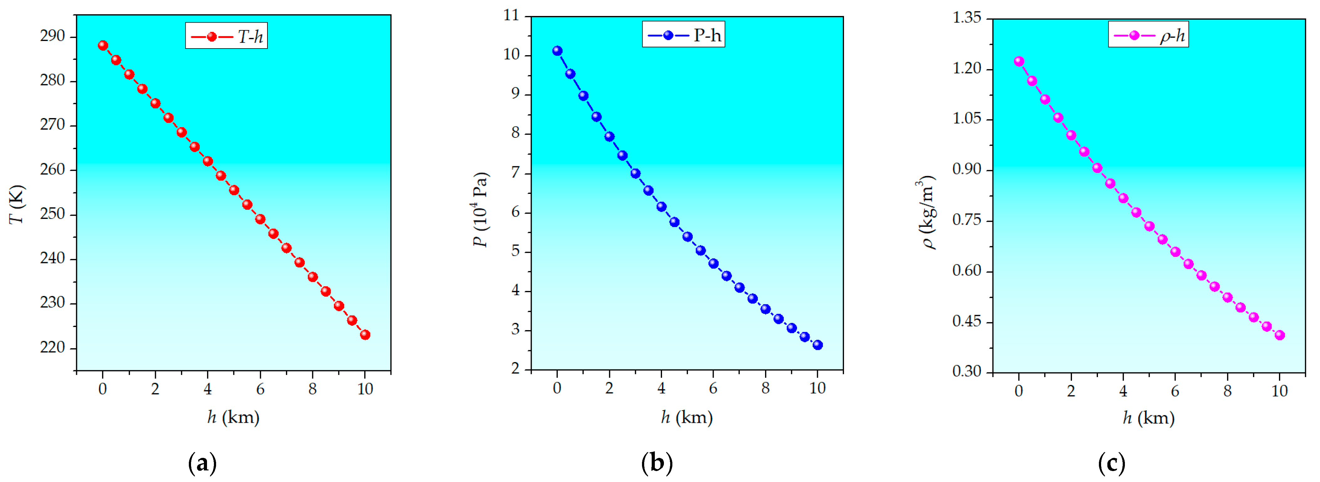
Therefore, according to the above formulas, the air state parameters corresponding to different altitudes could be obtained, as shown in

Table 1. The air state parameters at different altitudes.

Altitude h (km)	Temperature T (K)	Pressure P (104 Pa)	Density ρ (kg/m3)	Sound Velocity C (m/s)	Specific Internal Energy E (mJ/mg)	Viscosity μ (10−5 N·s/m2)
0.0	288.15	10.1325	1.225	340.29	206,786	1.8247
0.5	284.90	9.5461	1.167	338.37	204,453	1.8087
1.0	281.65	8.9875	1.112	336.43	202,121	1.7925
1.5	278.40	8.4556	1.058	334.48	199,789	1.7763
2.0	275.15	7.9495	1.006	332.53	197,456	1.7600
2.5	271.90	7.4683	0.957	330.56	195,124	1.7436
3.0	268.65	7.0109	0.909	328.57	192,792	1.7272
3.5	265.40	6.5764	0.863	326.58	190,460	1.7106
4.0	262.15	6.1640	0.819	324.57	188,127	1.6939
4.5	258.90	5.7728	0.777	322.56	185,795	1.6771
5.0	255.65	5.4020	0.736	320.53	183,463	1.6603
5.5	252.40	5.0507	0.697	318.48	181,130	1.6433
6.0	249.15	4.7181	0.660	316.42	178,798	1.6262
6.5	245.90	4.4035	0.624	314.35	176,466	1.6090
7.0	242.65	4.1061	0.590	312.27	174,133	1.5918
7.5	239.40	3.8251	0.557	310.17	171,801	1.5744
8.0	236.15	3.5600	0.525	308.06	169,469	1.5569
8.5	232.90	3.3099	0.495	305.93	167,137	1.5393
9.0	229.65	3.0742	0.466	303.79	164,804	1.5216
9.5	226.40	2.8524	0.439	301.63	162,472	1.5038
10.0	223.15	2.6436	0.413	299.46	160,140	1.4859

. For a more intuitive analysis, the relationship curves between air state parameters and altitude h are shown in Figure 1.

3. Numerical Simulation

3.1. Finite Element Model

As mentioned above, the space launch vehicle itself stores a large amount of liquid or solid propellant, which will release a huge amount of energy in the event of an explosion. In engineering practice, due to the different propellant types, the propellant is usually converted to a certain equivalent of TNT explosive. Thus, the problem of the accidental explosion of a space launch vehicle is transformed into a problem of TNT exploding in a free field. In dealing with TNT explosion problems, numerical simulations are usually carried out using AUTODYN software (v212) [27]. AUTODYN (Century Dynamics, Fort Worth, TX, USA) is an interactive nonlinear explicit dynamics analysis software, widely used in simulating detonation, impact, ballistics, and other problems [28]. The software has many excellent solvers, including Euler, Lagrange, ALE, SPH, and so on, as well as more than 300 commonly used material databases and complete fluid-structure coupling technology. The material model provided by AUTODYN software includes equations of state, strength model, and failure model.

The calculation accuracy and efficiency must be taken into account in numerical simulation of space vehicle explosions, due to the large area of the event. In two-dimensional or three-dimensional modeling of such a large area, the number of meshes will be very large, leading to a large demand on the computer simulation solving ability and a high time cost. Thus, one-dimensional wedge-shaped spherical symmetry was used to build the model, greatly reducing the total number of meshes compared with two-dimensional or three-dimensional modeling. When modeling, we set the mesh size to be very small and have encrypted the mesh, which not only ensured the accuracy of the simulation calculation, but also greatly improved the efficiency. In the finite element model, a TNT spherical charge was selected, the detonation method was center point detonation, and the non-reflective boundary condition was set at the boundary of the model. The mesh size was 1 mm and the total number of meshes was 10,000. Since the whole model involved two media, namely air and explosives, the Euler mesh was used in the modeling. In most of the empirical formulas of explosion shock waves, the proportional distance parameter z is introduced. The expression of the proportional distance is $z=r/\sqrt[3]{w}$, where r represents the distance from the monitoring point to the detonation center, in m, while w stands for the mass of the explosive, in kg. For the problem of an explosive free field explosion, as long as the proportional distance z is the same, the corresponding propagation law of the explosion shock wave will be the same. In this paper, the mass of TNT was set to 8 kg, and the value of r was set to 2~20 (the interval is 2 m); that is, the corresponding proportional distance z was 1~10 (the interval is 1). In order to facilitate subsequent analysis, a series of observation points were set in the finite element model. The entire finite element model is shown in Figure 2. A total of 21 groups of simulation conditions were carried out in this paper, corresponding to different altitudes (see Table 1).

3.2. Material Properties

When setting the parameters of the finite element model, the atmospheric environment corresponding to different altitudes was simulated by changing the initial state parameters of the air. The Ideal Gas equation of state in AUTODYN was selected as the equation of state for air, and the specific material parameters are shown in Table 1. The JWL (Jones–Wilkins–Lee) equation of state was chosen to describe the material properties of the TNT explosive. The JWL equation of state can accurately describe the volume, pressure, and energy characteristics of gas products in the process of detonation, its expression is as follows [29]:

$$P=A\left(1-\frac{\omega }{R_{1}V}\right)e^{-R_{1}V}+B\left(1-\frac{\omega }{R_{2}V}\right)e^{-R_{2}V}+\omega \rho E$$

(9)

where A, B, R₁, R₂, and w are material constants; V is the initial relative volume; E is the specific internal energy per mass; and P is the pressure. The specific parameters of TNT explosive are listed in

Table 2. The JWL parameters of TNT explosive.

Material	ρ (g/cm3)	A (GPa)	B (GPa)	R1	R2	ω	E (KJ/kg)
TNT	1.624	371.2	3.231	4.15	0.95	0.3	4290.0

. Based on the above parameter settings, the applicable range of the conclusions obtained from the later analysis is 1 ≤ z ≤ 10 and 0 km ≤ h ≤ 10 km.

4. Analysis of Numerical Simulation Results

When TNT explosive explodes in the air, it forms a mass of high temperature, high density, and high-pressure gas products. The gas products violently push against the stationary air around them, creating a series of compression waves that eventually add up to form a shock wave. Due to the limited work distance of gas products during external expansion, and the rapid decay in the expansion process, the change of temperature and density will only be concerned when studying the central reaction region. However, for explosive problems, we usually focus on targets outside the central reaction area of the explosive, such as buildings, equipment, and personnel. The damage to various targets under explosion is extremely complex, and the parameters used to measure the explosion shock wave mainly include the peak overpressure ΔP, positive pressure action time t+, and specific impulse i. In engineering applications, the shock wave peak overpressure ΔP is often used as a criterion to classify the damage degree of the target. Taking personnel as an example, the damage degree caused by shock wave overpressure to exposed personnel is as follows [30]: slight damage (0.02 MPa ≤ ΔP ≤ 0.03 MPa), moderate damage (0.03 MPa ≤ ΔP ≤ 0.05 MPa), serious damage (0.05 MPa ≤ ΔP ≤ 0.1 MPa), and death (ΔP ≥ 0.1 MPa). Therefore, this paper did not take temperature, density, and other parameters as the research objects, but took shock wave pressure as the main research object.

After completing the numerical simulation solution, the pressure nephogram and pressure–time history curve of explosion shock wave propagation under each working condition was obtained. In order to display and analyze the simulation results of each working condition more intuitively, three groups of working conditions (h = 0 km, h = 5 km, and h = 10 km) were selected as representative for illustration in this paper. Figure 3 shows the pressure nephogram of explosion shock wave propagation at different moments of the three groups of working conditions; (a)~(e) corresponds to the altitude h = 0 km, (f)~(j) corresponds to the altitude h = 5 km, and (k)~(o) corresponds to the altitude h = 10 km. Figure 4 shows the pressure–time history curve of the three groups of working conditions. Due to the #1 observation point being close to the explosion center, its pressure peak was very high. In addition, the explosion shock wave attenuated rapidly when it propagated in the free field, so the pressure peaks at the other observation points were small. As a result, the pressure–time history curve of the other observation points under the same pressure ordinate appeared relatively flat compared with the #1 observation point, especially the #6~#10 observation points. In order to visualize the pressure–time history curve of the #6~#10 observation points more clearly, the pressure–time history curves of the #6~#10 observation points were locally enlarged in Figure 4.

When analyzing the pressure–time history curve of each group of working conditions, the peak pressure of each observation point could be obtained by extracting the maximum value of the pressure–time history curve, as shown in

Table 3. Peak pressure of each observation point at different altitudes.

Altitude h (km)	Peak Pressure P (KPa)
	#1	#2	#3	#4	#5	#6	#7	#8	#9	#10
0.0	1104.4	287.89	181.63	148.8	133.87	125.59	120.44	116.96	114.48	112.63
0.5	1088.1	279.26	174.04	141.74	127.11	119.03	114.01	110.61	108.19	106.39
1.0	1072.5	271.25	166.82	135.07	120.74	112.84	107.93	104.62	102.27	100.52
1.5	1056.2	263.37	159.89	128.61	114.55	106.83	102.04	98.822	96.532	94.83
2.0	1040.1	255.86	153.17	122.41	108.64	101.12	96.429	93.294	91.064	89.409
2.5	1024.4	248.76	146.92	116.57	103.11	95.724	91.166	88.111	85.942	84.333
3.0	1008.1	241.92	140.81	110.94	97.727	90.523	86.078	83.102	80.992	79.428
3.5	991.74	235.36	134.99	105.57	92.613	85.573	81.243	78.346	76.293	74.773
4.0	974.58	229.16	129.47	100.46	87.757	80.883	76.657	73.837	71.84	70.363
4.5	959.22	223.27	124.21	95.624	83.161	76.438	72.317	69.571	67.627	66.192
5.0	942.61	217.59	119.13	90.925	78.721	72.149	68.131	65.458	63.57	62.177
5.5	925.45	212.19	114.32	86.501	74.524	68.121	64.183	61.581	59.745	58.391
6.0	908.56	207.11	109.76	82.321	70.558	64.285	60.464	57.931	56.146	54.831
6.5	890.74	202.21	105.38	78.293	66.753	60.614	56.89	54.424	52.691	51.414
7.0	874.28	197.61	101.28	74.501	63.164	57.171	53.537	51.139	49.453	48.213
7.5	856.19	193.19	97.311	70.857	59.724	53.866	50.323	47.991	46.351	45.149
8.0	838.29	189.19	93.499	67.358	56.426	50.696	47.245	44.975	43.384	42.218
8.5	819.62	185.22	89.961	64.087	53.349	47.741	44.377	42.167	40.622	39.49
9.0	801.91	181.47	86.566	60.955	50.401	44.913	41.635	39.485	37.986	36.888
9.5	783.37	177.91	83.421	58.048	47.666	42.294	39.095	37.003	35.547	34.481
10.0	765.44	174.49	80.415	55.265	45.059	39.801	36.678	34.642	33.226	32.193

.

It is generally believed that the peak overpressure ΔP of a shock wave is a function of the proportional distance z. On this basis, many experts have conducted experimental studies and summarized a variety of empirical formulas. The typical empirical formulas of shock wave pressure include Henrych’s formula [7], Sadovskyi’s formula [8], Brode’s formula [9], Aliansov’s formula [10], and Baker’s formula [11]. Through comparative analysis, it could be seen that these empirical formulas for calculating the shock wave pressure are all functions of the proportional distance z, and the power exponent of z is no more than the third-order exponent. Taking Henrych’s formula and Sadovskyi’s formula as examples, when the proportional distance z is 1~10, the expression of Henrych’s formula (MPa) is

$$\Delta P=\frac{0.0662}{z}+\frac{0.405}{z^2}+\frac{0.3288}{z^3}$$

(10)

and the expression of Sadovskyi’s formula (MPa) is

$$\Delta P=\frac{0.076}{z}+\frac{0.255}{z^2}+\frac{0.65}{z^3}$$

(11)

Many experts [31,32] have analyzed the differences between these empirical formulas of shock wave overpressure, and found that there are some deviations between them, and that the scope of application has not been consistent. During the research process, we conducted third-order and fourth-order fitting on the proportional distance z of the numerical simulation results. We found that the fourth-order fitting degree was higher, and the error between them and the experimental data was smaller. Therefore, this paper adopted fourth-order fitting when processing the numerical simulation data. By fitting the peak pressures of each observation point, the fitting curves of the peak pressures of each observation point at different altitudes were obtained, and are shown in Figure 5.

The model between the pressure peak P and proportional distance z established in this paper was as follows:

$$P=a/z+b/z^2+c/z^3+d/z^4+P_h$$

(12)

R-Square is mathematically defined as the Coefficient of Determination, which is a parameter to measure the fit degree of a model and mainly applies to a single variable. If there are multiple variables in the model, the applicability and accuracy of R-Square will be reduced. In this case, in order to ensure the accuracy of the evaluation model, it was necessary to introduce Adj. R-Square. The normal value range of Adj. R-Square is 0~1, and the closer it is to 1, the better the data fitting effect of the constructed model is. It can be seen from Figure 5 that the Adj. R-Square values of the relationship curve obtained by fitting 21 groups of working conditions were all 1, which indicated that the fitting degree of the model was very high and better reflected the accuracy of the model.

In the analysis of the fitting relationship of each group of working conditions, it was found that the parameters a, b, c, d and P_h in Formula (12) were all related to the altitude h. A change of altitude led to change in these four parameters. The relationship between P₀ and P_h was clear, and is shown in Formula (5). Therefore, the values of the fitting parameters a, b, c, d at different altitudes are shown in

Table 4. The values of fitting parameters a, b, c, d at altitude h.

Altitude h (km)	a	b	c	d
0.0	0.79024	3.07608	5.05003	1.11442
0.5	0.76786	2.90715	5.37483	0.87657
1.0	0.75353	2.62496	5.96283	0.47494
1.5	0.7394	2.47172	6.29346	0.20987
2.0	0.72312	2.2519	6.78314	−0.1531
2.5	0.71624	2.01453	7.28512	−0.5187
3.0	0.70089	1.80673	7.76993	−0.89763
3.5	0.68849	1.58743	8.27968	−1.29583
4.0	0.67978	1.3481	8.85634	−1.75481
4.5	0.67402	1.10683	9.41767	−2.18358
5.0	0.66238	0.87995	9.99274	−2.64925
5.5	0.65463	0.64497	10.58562	−3.13577
6.0	0.65312	0.37807	11.25108	−3.66847
6.5	0.64545	0.14216	11.87781	−4.19834
7.0	0.64148	−0.09351	12.4855	−4.70127
7.5	0.63631	−0.34158	13.1619	−5.27722
8.0	0.63224	−0.62832	13.98584	−5.96284
8.5	0.62843	−0.86687	14.65456	−6.55109
9.0	0.62212	−1.09554	15.31467	−7.12954
9.5	0.6212	−1.32909	15.96843	−7.71205
10.0	0.61819	−1.54884	16.59549	−8.27478

, and the fitting curves of the relationship between the parameters a, b, c, d and the altitude h were obtained, as shown in Figure 6.

As can be seen from Figure 6, the corresponding Adj. R-Square values of the parameters a, b, c and d were 0.99684, 0.9997, 0.99967, and 0.99976, respectively, all of which were very close to 1, indicating that the fitting degree of these four coefficients was high. Therefore, the specific expressions of parameters a, b, c, d and altitude h were obtained as follows:

$$a=0.78431-0.03176h+0.00155h^2$$

(13)

$$b=3.09964-0.42227h-0.00476h^2$$

(14)

$$c=4.99716+0.8332h+0.03417h^2$$

(15)

$$d=1.142-0.57233h-0.03801h^2$$

(16)

As a result, the rapid evaluation formula for the peak pressure of explosion shock wave at different altitudes could be obtained. Since the altitude h studied in this paper was 0~10 km, and the proportional distance z was 1~10, in order to ensure the scientificity and accuracy, it was necessary to limit the scope of application of the rapid evaluation formula. The specific expression of the rapid evaluation formula was as follows:

$$\left\{\begin{array}{l}P=a/z+b/z^2+c/z^3+d/z^4+P_h\left[h\in (0\mathrm{km},10\mathrm{km});z\in (1,10)\right]\\ a=0.78431-0.03176h+0.00155h^2\\ b=3.09964-0.42227h-0.00476h^2\\ c=4.99716+0.8332h+0.03417h^2\\ d=1.142-0.57233h-0.03801h^2\\ P_h={\left(\frac{288.15-6.5h}{288.15}\right)}^{5.25588}{P}_0\left[P_0=1.01325\mathrm{bar};(1\mathrm{bar}={10}^5\mathrm{P}\mathrm{a})\right]\end{array}\right.$$

(17)

For the equation $P=a/z+b/z^2+c/z^3+d/z^4+P_h$, the left side is a parameter that we want to obtain, and the right side can degenerate into the parameters related to h, r, and w. For a specific space launch vehicle, the equivalent TNT mass w is known. As long as the altitude h is determined, the explosion shock wave pressure at different distances r can be rapidly obtained; that is, the propagation law of the explosion shock wave can be obtained. Therefore, the relationship between the explosion shock wave parameters and the altitude was found to be very close.

5. Experimental Verification of the Rapid Evaluation Formula

In order to verify the rapid evaluation formula of explosion shock wave pressure obtained in this paper, it was necessary to compare the calculated value obtained from the formula with the measured value obtained from the experiments. Considering the experimental cost and period, this paper took the experimental results obtained by Chen [21] as reference. In order to study the influence of different low-pressure environments on explosion shock waves, they measured the explosion shock wave pressure of TNT explosives in a sealed tank by simulating the plateau low-pressure environment in the sealed tank with an air pumping device.

The sealed tank used by Chen in the experiment has a body length of 2.8 m, a diameter of 2 m, a volume of 7.3 m³, and a designed maximum working pressure of 6 MPa. The schematic diagram of the experimental device is shown in Figure 7. The experimental system included the initiation system, pressure testing system, and low-pressure environment simulation system. The initiation system was composed of a synchronous machine, high voltage pulse generator and a detonator. The pressure testing system included a free field shock wave sensor arranged in the tank and its matching signal adjuster and a data recorder. After detonation, the pressure signal measured by the sensor was transmitted to the signal adjuster, and the micro charge signal obtained by the sensor was amplified and finally stored by the data recorder. The low-pressure environment simulation system consisted of a vacuum pump and a pressure monitoring device. By using the vacuum pump to draw air from the tank to create a low-pressure environment, the pressure could be adjusted according to the pressure monitor reading to achieve the pressure level required by the experiment.

Spherical TNT explosive was used in the experiment, and the initiation mode was center initiation. The TNT explosive was divided into the upper and lower hemispheres. A groove was reserved in the lower hemisphere to place the booster charge, and a detonator placement hole was prefabricated in the upper hemisphere. The upper and lower hemispheres were bonded with glue before initiation, and the spherical charge was hoisted at a predetermined position and fixed after being combined. The sensor was welded to the steel plate at the bottom of the tank body through a screw. The height of the sensor and the direction of the sensitive surface could be adjusted through the fixing nut at the top of the screw. During installation, the direction could be adjusted so that the shock wave front was perpendicular to the disk plane. The height of the sensor could be adjusted to avoid the impact of the Mach wave formed on the ground and the reflected wave formed by the other walls on the incident shock wave, so as to ensure that the sensor could completely record the pressure–time history data of the positive pressure area of the incident wave. The distribution of measuring points of the pressure sensor is shown in Figure 8, and the numbering of measurement points from left to right is #1~#6.

Before the experiment, the sensor was dynamically calibrated with 1 kg standard spherical charge. In the formal experiment, spherical charges with radius R = 35 mm and R = 25 mm were selected, and the weights of the two spherical charges were 292 g and 106 g, respectively. The initial ambient pressure in the tank was set to 95 KPa, 74 KPa, and 57 KPa, respectively, corresponding to the atmospheric pressure at the altitude h = 0.5 km, 2.5 km, and 4.5 km. In order to ensure the validity of the test data, each different weight explosive was tested twice under different pressure conditions. This was to ensure data were not missed, and allowed the two sets of data to be verified against each other. Therefore, under the experimental conditions of the three altitudes, two types of explosives, and six observation points, 72 sets of experimental data were obtained.

The explosion shock wave overpressure peaks at different proportional distances at three altitudes, h= 0.5 km, 2.5 km, and 4.5 km, were obtained through the tests. Since there were 72 sets of experimental data in total, 42 representative sets of experimental data were selected for more efficient analysis. These 42 sets of data corresponded to 292 g (#2, #5, #6) and 106 g (#1, #3, #5, #6), respectively. These 42 sets of experimental data better covered the proportional distances from 1.2 to 2.6, and the spacing of the proportional distances was relatively uniform. The explosion shock wave overpressure peaks at different proportional distances could also be calculated based on the rapid evaluation Formula (10). The experimental and calculated values, as well as the errors between them, are shown in

Table 5. The explosion shock wave overpressure peaks at different proportional distances.

Altitude h (km)	Test Condition	Actual Proportional Distance z (m/kg1/3)	Experimental Value ΔPe (KPa)	Mean Value ΔP’e (KPa)	Calculated Value ΔPc (KPa)	Error (%) (ΔP’e − ΔPc)/ΔP’e
0.5	292 g (#2)	1.16	677.28	688.13	648.19	5.80
			698.98
	106 g (#1)	1.37	460.59	457.93	444.85	2.85
			455.27
	292 g (#5)	1.60	323.46	318.93	306.13	4.01
			314.39
	292 g (#6)	1.82	240.02	241.64	229.93	4.85
			243.26
	106 g (#3)	2.01	191.92	183.00	181.67	0.73
			174.07
	106 g (#5)	2.29	141.17	137.75	136.86	0.65
			134.32
	106 g (#6)	2.61	107.12	103.84	104.16	−0.31
			100.56
2.5	292 g (#2)	1.18	639.08	629.47	621.98	1.19
			619.86
	106 g (#1)	1.37	432.12	440.03	420.56	4.42
			447.93
	292 g (#5)	1.61	296.57	300.61	289.03	3.85
			304.65
	292 g (#6)	1.81	211.89	222.02	219.06	1.33
			232.14
	106 g (#3)	2.05	170.30	166.89	164.46	1.46
			163.47
	106 g (#5)	2.29	135.57	134.03	128.43	4.18
			132.49
	106 g (#6)	2.60	98.57	98.41	97.62	0.81
			98.26
4.5	292 g (#2)	1.20	588.55	576.44	572.62	0.66
			564.32
	106 g (#1)	1.43	362.84	375.78	371.07	1.25
			388.72
	292 g (#5)	1.64	282.37	268.66	265.55	1.16
			254.95
	292 g (#6)	1.84	214.32	212.63	201.43	5.27
			210.94
	106 g (#3)	1.99	169.17	170.77	167.38	1.99
			172.36
	106 g (#5)	2.30	124.17	122.32	119.81	2.05
			120.46
	106 g (#6)	2.62	90.43	91.63	89.55	2.27
			92.82

. In order to analyze the experiment and calculation results more intuitively, we presented the experiment results in the form of bar charts and error bars, and presented the errors between the experiment and calculation results in the form of line charts, as shown in Figure 9.

In each working condition, we analyzed two sets of parallel experimental data, comparing and analyzing the data obtained from two tests under the same working conditions to ensure the validity of the test data. Due to the interference of various factors during the collection process of the experimental data, we cannot guarantee that the environment, data collection, data reading, and other aspects of the two experiments were absolutely identical. Based on the analysis of Table 5 and Figure 9, the following conclusions can be drawn:

(1)

At the same measuring point, for the same weight explosives, the deviation of the measured experimental data was relatively small and within an acceptable range.

(2)

At different altitudes, the overpressure of explosion shock waves exhibited a rapid attenuation pattern with an increasing proportional distance, which is very consistent with the propagation characteristics of explosion shock waves.

(3)

The error range between the calculated value obtained by the rapid evaluation formula and the measured value was less than 5.80%, which demonstrated that the rapid evaluation formula obtained in this paper is scientific and reasonable.

Through the above comparative verification, it can be seen that the rapid evaluation formula established in this paper has good rationality. However, we need to pay attention to the prerequisite conditions for the application of this formula. Since we are mainly concerned about the troposphere (0–10 km) in this paper, which may have a serious impact on human safety, the research of the entire paper focuses on the altitude between 0–10 km. The premise of this paper has been explained in Section 2. If the altitude exceeds this range, it is necessary to modify the rapid evaluation formula based on this research method to expand its applicability.

6. Conclusions

The accidental explosion of space launch vehicles is an important research issue. In order to establish a rapid evaluation method for the destructive power of an explosive in different atmospheric environments, we conducted extensive simulation analysis using AUTODYN software. When analyzing the simulation results, we found that there is a relationship between the explosion shock wave pressure and the altitude. Based on the simulation data, the rapid evaluation formula of explosion shock wave pressure at different altitudes was obtained, as shown below:

$$\left\{\begin{array}{l}P=a/z+b/z^2+c/z^3+d/z^4+P_h\left[h\in (0\mathrm{km},10\mathrm{km});z\in (1,10)\right]\\ a=0.78431-0.03176h+0.00155h^2\\ b=3.09964-0.42227h-0.00476h^2\\ c=4.99716+0.8332h+0.03417h^2\\ d=1.142-0.57233h-0.03801h^2\\ P_h={\left(\frac{288.15-6.5h}{288.15}\right)}^{5.25588}{P}_0\left[P_0=1.01325\mathrm{bar};(1\mathrm{bar}={10}^5\mathrm{Pa})\right]\end{array}\right.$$

In addition, the test results showed that the error range between the calculated value and the test value was less than 5.80%, verifying the scientificity and rational qualities of the rapid evaluation formula. This formula has significant theoretical and engineering value. In terms of theoretical analysis, it can effectively compensate for the limitations of existing traditional empirical formulas. In engineering applications, it can be used to rapidly evaluate the destructive power of space launch vehicles after accidental explosions, to support the analysis of explosion safety distances for space launch sites.