
Design of Flyby Trajectories with Powered Gravity and Aerogravity Assist Maneuvers
Abstract
:1. Introduction
2. Background
2.1. Dynamical Model
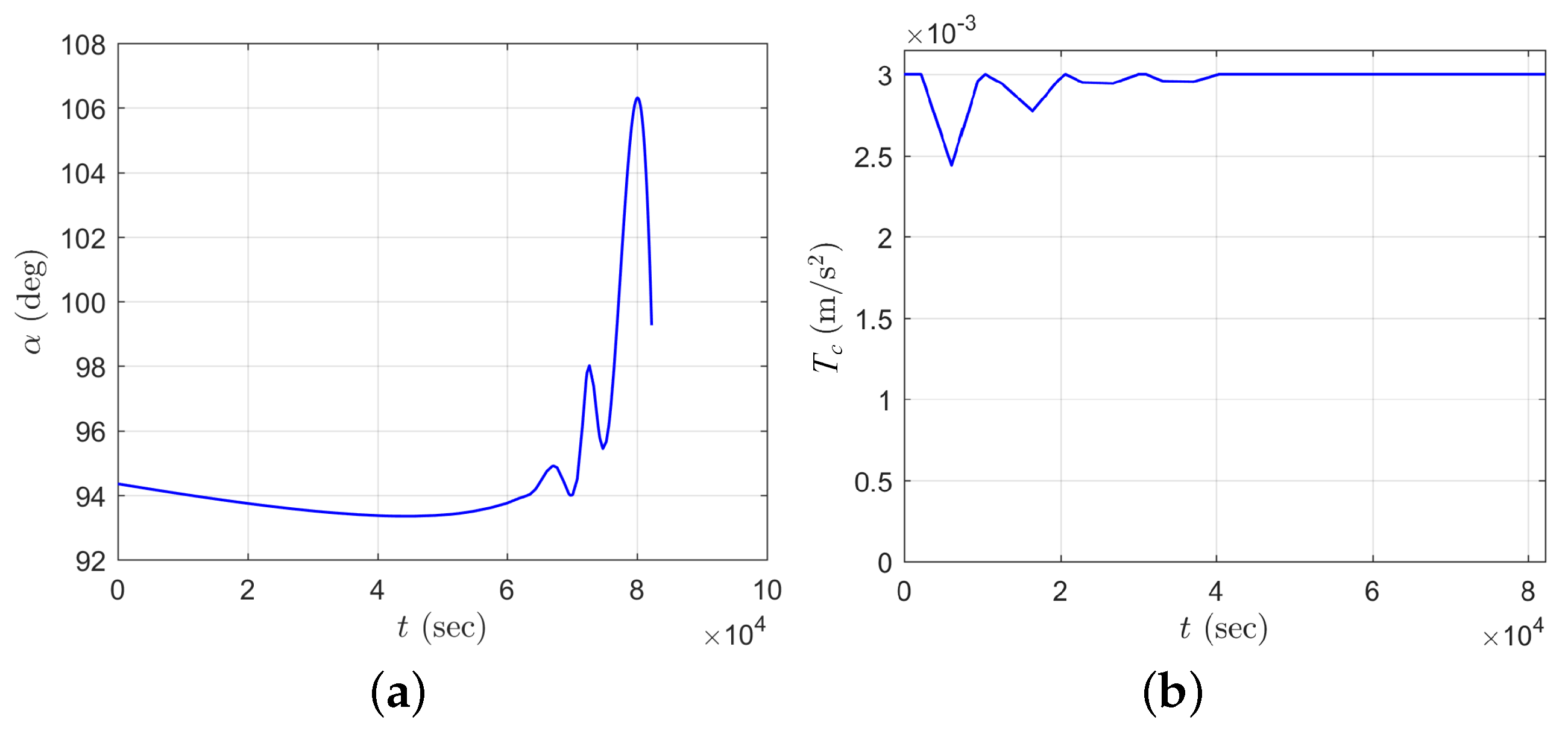
2.2. PGA Portion
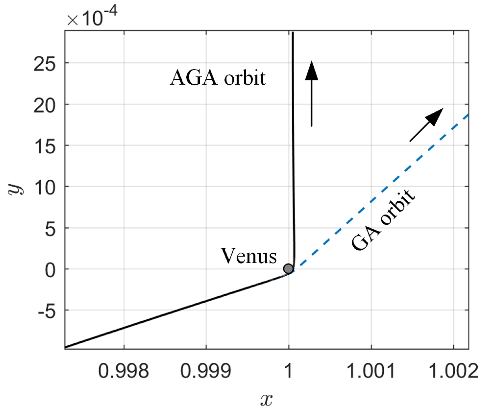
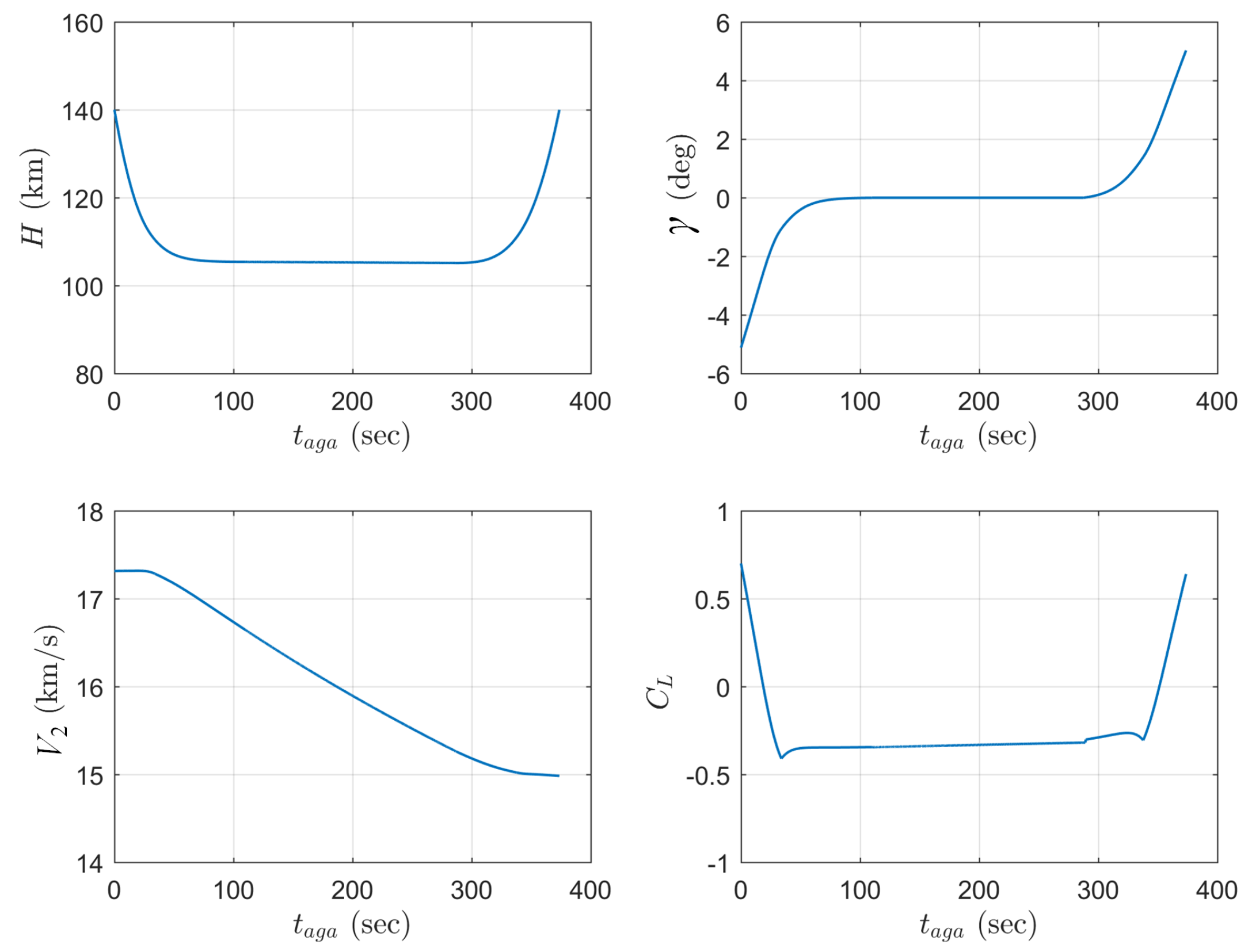
3. AGA Portion
3.1. Flight-Path Angle Guidance Algorithm
3.2. Comparison of AGA Portion
4. Results and Discussion
4.1. Case of
4.2. Case of
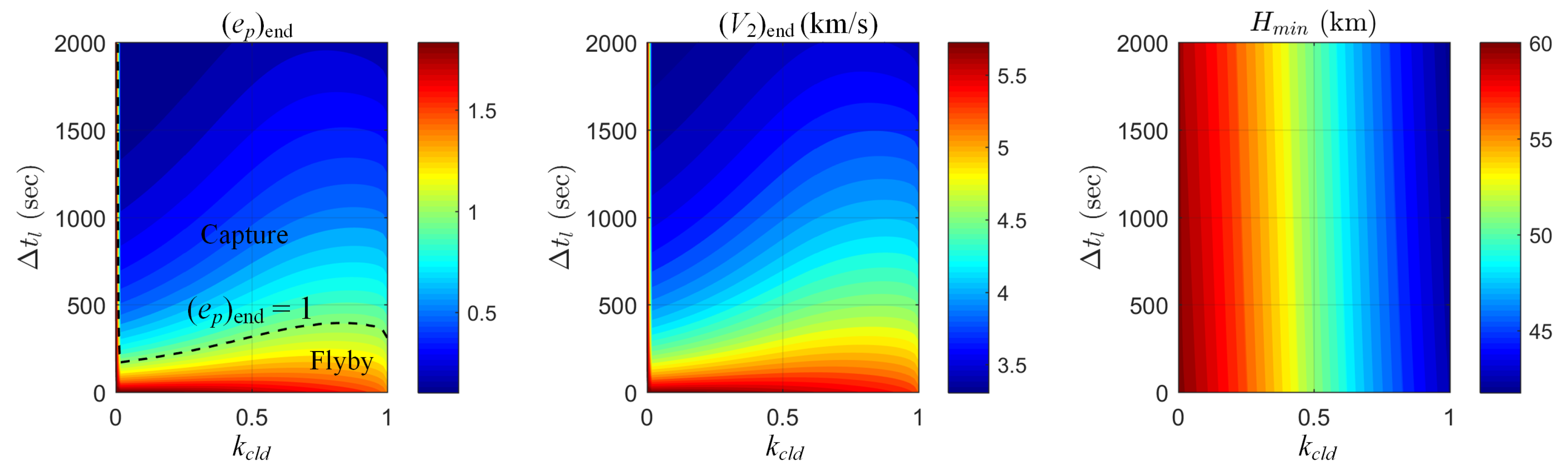
4.3. Influence of Elliptic Model
5. Conclusions
Author Contributions
Funding
Data Availability Statement
Conflicts of Interest
Abbreviations
| AGA | Aerogravity assist |
| PGA | Powered gravity assist |
| PERTBP | Planar elliptic restricted three-body problem |
| GA | Gravity assist |
| PSB | Powered swing-by |
| CRTBP | Circular restricted three-body problem |
References
- Prado, A.F.B. Powered swingby. J. Guid. Control. Dyn. 1996, 19, 1142–1147. [Google Scholar] [CrossRef]
- Casalino, L.; Colasurdo, G.; Pastrone, D. Simple strategy for powered swingby. J. Guid. Control. Dyn. 1999, 22, 156–159. [Google Scholar] [CrossRef]
- Ferreira, A.F.; Prado, A.F.; Winter, O.C. A numerical mapping of energy gains in a powered Swing-By maneuver. Nonlinear Dyn. 2017, 89, 791–818. [Google Scholar] [CrossRef]
- Ferreira, A.F.; Prado, A.F.; Winter, O.C.; Santos, D.P. Effects of the eccentricity of the primaries in powered Swing-By maneuvers. Adv. Space Res. 2017, 59, 2071–2087. [Google Scholar] [CrossRef]
- Qi, Y.; de Ruiter, A. Powered Swing-By with Continuous Thrust. J. Guid. Control. Dyn. 2020, 43, 111–121. [Google Scholar] [CrossRef]
- Miele, A.; Wang, T. Gamma guidance of trajectories for coplanar, aeroassisted orbital transfer. J. Guid. Control. Dyn. 1992, 15, 255–262. [Google Scholar] [CrossRef]
- McRonald, A.D.; Randolph, J.E. Hypersonic maneuvering for augmenting planetary gravity assist. J. Spacecr. Rocket. 1992, 29, 216–222. [Google Scholar] [CrossRef]
- Lohar, F.A.; Misra, A.K.; Mateescu, D. Optimal atmospheric trajectory for aerogravity assist with heat constraint. J. Guid. Control. Dyn. 1995, 18, 723–730. [Google Scholar] [CrossRef]
- Johnson, W.R.; Longuski, J.M. Design of aerogravity-assist trajectories. J. Spacecr. Rocket. 2002, 39, 23–30. [Google Scholar] [CrossRef]
- Pessina, S.M.; Campagnola, S.; Vasile, M. Preliminary analysis of interplanetary trajectories with aerogravity and gravity assist manoeuvres. In Proceedings of the 54th International Astronautical Congress, Bremen, Germany, 29 September–3 October 2003. [Google Scholar]
- Mazzaracchio, A. Flight-Path Angle Guidance for Aero-Gravity Assist Maneuvers on Hyperbolic Trajectories. J. Guid. Control. Dyn. 2015, 38, 238–248. [Google Scholar] [CrossRef]
- Han, H.; Qiao, D.; Chen, H. Optimal ballistic coefficient control for Mars aerocapture. In Proceedings of the 2016 IEEE Chinese Guidance, Navigation and Control Conference (CGNCC), Nanjing, China, 12–14 August 2016; IEEE: New York, NY, USA, 2016; pp. 2175–2180. [Google Scholar] [CrossRef]
- Han, H.; Li, X.; Qiao, D. Aerogravity-assist capture into the three-body system: A preliminary design. Acta Astronaut. 2022, 198, 26–35. [Google Scholar] [CrossRef]
- Zhang, G.; Wen, C.; Han, H.; Qiao, D. Aerocapture Trajectory Planning Using Hierarchical Differential Dynamic Programming. J. Spacecr. Rocket. 2022, 59, 1647–1659. [Google Scholar] [CrossRef]
- Piñeros, J.O.M.; de Almeida Prado, A.F.B. Powered aero-gravity-assist maneuvers considering lift and drag around the Earth. Astrophys. Space Sci. 2017, 362, 120. [Google Scholar] [CrossRef]
- Qi, Y.; de Ruiter, A. Optimal Powered Aerogravity-Assist Trajectories. J. Guid. Control. Dyn. 2021, 44, 151–162. [Google Scholar] [CrossRef]
- Szebehely, V. Theory of Orbit: The Restricted Problem of Three Bodies; Academic Press: Cambridge, MA, USA, 1967; pp. 587–597. [Google Scholar]
- Ferreira, A.F.; Prado, A.F.; Winter, O.C.; Santos, D.P. Analytical study of the swing-by maneuver in an elliptical system. Astrophys. Space Sci. 2018, 363, 24. [Google Scholar] [CrossRef]
- Qi, Y.; de Ruiter, A. Energy analysis in the elliptic restricted three-body problem. Mon. Not. R. Astron. Soc. 2018, 478, 1392–1402. [Google Scholar] [CrossRef]
- Qi, Y.; de Ruiter, A. Powered Swing-by in the Elliptic Restricted Three-body Problem. Mon. Not. R. Astron. Soc. 2018, 481, 4621–4636. [Google Scholar] [CrossRef]
- Bate, R.R.; Mueller, D.D.; White, J.E. Fundamentals of Astrodynamics; Courier Corporation: Chelmsford, MA, USA, 1971; pp. 333–334. [Google Scholar]
- Henning, G.A.; Edelman, P.J.; Longuski, J.M. Design and optimization of interplanetary aerogravity-assist tours. J. Spacecr. Rocket. 2014, 51, 1849–1856. [Google Scholar] [CrossRef]
- Lohar, F.A.; Mateescu, D.; Misra, A. Optimal atmospheric trajectory for aero-gravity assist. Acta Astronaut. 1994, 32, 89–96. [Google Scholar] [CrossRef]
- Havey, K.A., Jr. Entry vehicle performance in low-heat-load trajectories. J. Spacecr. Rocket. 1982, 19, 506–512. [Google Scholar] [CrossRef]
- Tauber, M.E.; Sutton, K. Stagnation-point radiative heating relations for Earth and Mars entries. J. Spacecr. Rocket. 1991, 28, 40–42. [Google Scholar] [CrossRef]
- Edelman, P.J.; Longuski, J.M. Optimal Aerogravity-Assist Trajectories Minimizing Total Heat Load. J. Guid. Control. Dyn. 2017, 40, 2699–2703. [Google Scholar] [CrossRef]
- Koon, W.S.; Lo, M.W.; Marsden, J.E.; Ross, S.D. Dynamical Systems, the Three-Body Problem and Space Mission Design; World Scientific: Singapore, 2000; pp. 97–100. [Google Scholar] [CrossRef]
- Lantoine, G.; Russell, R.P. Near ballistic halo-to-halo transfers between planetary moons. J. Astronaut. Sci. 2011, 58, 335–363. [Google Scholar] [CrossRef]
- Canales, D.; Howell, K.C.; Fantino, E. Moon-to-moon transfer methodology for multi-moon systems in the coupled spatial circular restricted three-body problem. In Proceedings of the AAS/AIAA Astrodynamics Specialist Conference, South Lake Tahoe, CA, USA, 9–13 August 2020; Volume 8. [Google Scholar]
- Fantino, E.; Burhani, B.; Flores, R.; Alessi, E.; Solano, F.; Sanjurjo-Rivo, M. End-to-end trajectory concept for close exploration of Saturn’s Inner Large Moons. Commun. Nonlinear Sci. Numer. Simul. 2023, 126, 107458. [Google Scholar] [CrossRef]


| Method | (km/s) | (km/s) | (km/s) | (km) | (km/s) | (deg) | (s) |
|---|---|---|---|---|---|---|---|
| Ours | 14 | 10.99 | 15.66 | 105.14 | 17.32 | 73.44 | 373.65 |
| Ref. [11] | 14 | 11.76 | 15.60 | 110.10 | 17.36 | 73.95 | 375.91 |
| Name | Symbol | Value |
|---|---|---|
| Mass ratio of ERTBP | 3.253253 | |
| Mass coefficient | 1.327128 km3/s2 | |
| Semi-major axis of ERTBP | a | 2.2792 km |
| Eccentricity of ERTBP | e | 0.0935 |
| Radius of Mars | 3396.2 km | |
| Radius of SOI | 5.7914 km | |
| Reference density | 0.02 kg/m3 | |
| Inverse scale altitude | 0.094 km−1 | |
| Sensible altitude of atmosphere | 500 km | |
| Vehicle mass | m | 1500 kg |
| Aerodynamic reference area | S | 30 m2 |
| Maximum lift-to-drag ratio | 3 | |
| Lift coefficient at maximum | 0.034 | |
| Sutton-Graves constant | 1.9027 (m)/cm2 | |
| Nose radius | 1 m | |
| Maximum | 0.7 | |
| Maximum thrust acceleration | 0.003 m/s2 | |
| Initial eccentricity | 4.5 | |
| True anomaly of the periapsis | 0 deg | |
| Initial periapsis altitude | 10,000 km | |
| Target periapsis altitude | 60 km |
| Orbit | (s) | (km/s) | (km2/s2) | (deg) | ||
|---|---|---|---|---|---|---|
| GA orbit | – | – | 4.4994 | 1.5959 | 25.6384 | |
| PGA orbit | – | – | 2.0426 | 3.4067 | 61.8849 | |
| PGA+AGA orbit 1 | 0.82 | 142 | 1.3412 | 3.9754 | 104.2773 | |
| PGA+AGA orbit 2 | 0.3 | 0 | 1.8183 | 3.6915 | 71.2620 | |
| PGA+AGA orbit 3 | 0.83 | 393 | 1.0081 | 2.7968 | 159.2501 |
| Orbit | (s) | (km/s) | (km2/s2) | (deg) | ||
|---|---|---|---|---|---|---|
| GA orbit | – | – | 4.4994 | 1.5959 | 40.0741 | 25.6384 |
| PGA orbit | – | – | 2.0426 | 3.7093 | 89.3518 | 61.8850 |
| PGA+AGA orbit 1 | 0.9 | 386 | 1.0092 | 5.2370 | 23.6754 | 159.3214 |
| PGA+AGA orbit 2 | 0.15 | 0 | 1.8571 | 4.0576 | 93.3228 | 69.3531 |
Disclaimer/Publisher’s Note: The statements, opinions and data contained in all publications are solely those of the individual author(s) and contributor(s) and not of MDPI and/or the editor(s). MDPI and/or the editor(s) disclaim responsibility for any injury to people or property resulting from any ideas, methods, instructions or products referred to in the content. |
© 2024 by the authors. Licensee MDPI, Basel, Switzerland. This article is an open access article distributed under the terms and conditions of the Creative Commons Attribution (CC BY) license (https://creativecommons.org/licenses/by/4.0/).
Share and Cite
Yu, W.; Qi, Y. Design of Flyby Trajectories with Powered Gravity and Aerogravity Assist Maneuvers. Aerospace 2024, 11, 129. https://doi.org/10.3390/aerospace11020129
Yu W, Qi Y. Design of Flyby Trajectories with Powered Gravity and Aerogravity Assist Maneuvers. Aerospace. 2024; 11(2):129. https://doi.org/10.3390/aerospace11020129
Chicago/Turabian StyleYu, Wanze, and Yi Qi. 2024. "Design of Flyby Trajectories with Powered Gravity and Aerogravity Assist Maneuvers" Aerospace 11, no. 2: 129. https://doi.org/10.3390/aerospace11020129