Global Surface Pressure Pattern for a Compressible Elliptical Cavity Flow Using Pressure-Sensitive Paint

Abstract

The flow field in a cavity depends on the properties of the upstream boundary layer and the cavity geometry. Comprehensive studies for rectangular cavities have been conducted. This experimental study determines the global surface pressure pattern for elliptical cavities (eccentricities of 0, 0.66 and 0.87) in a naturally developed turbulent boundary layer using pressure-sensitive paint. The ratio between the length (major axis) and the depth is 4.43–21.5, and the freestream Mach number is 0.83. The mean surface pressure distribution of an elliptical cavity resembles that of a rectangular cavity. A change in the value of eccentricity (wall curvature) affects the region for an adverse pressure gradient in an open cavity, an extension of the plateau in a transitional–closed cavity and flow expansion near the front and rear edges. The boundaries between an open, transitional and closed cavities vary.

1. Introduction

Cavities are common on aerodynamic vehicles in landing gear wells and in weapon bays. Flow characteristics depend on cavity geometry, wind direction and the properties of the upstream boundary layer (laminar or turbulent, the Reynolds number and the freestream Mach number, M) [1,2,3,4]. Numerous studies involve a two-dimensional rectangular cavity flow. The ratio between the length and the depth, L/H, is the key parameter affecting the flow. The classic definition of different flow regimes (open, transitional and closed) was provided by Charwat et al. [5]. For an open cavity, the value of L/H is less than 6–8 in subsonic and transonic speed regimes [6,7]. The incoming boundary layer separates at the front edge and forms vortices due to the Kelvin–Helmholtz instability. A shear layer bridges the cavity, and a vortex forms inside the cavity. There is a uniform streamwise pressure distribution on the cavity floor. A feedback loop is caused by an unsteady shear layer and the upstream propagation of pressure waves at the rear wall, so self-sustained oscillations result in noise emission and intense pressure fluctuations. Non-harmonic modal frequencies or discrete tones are determined using the Rossiter–Heller empirical formula [8,9]. If the value of L/H exceeds 9–15 [6,7], a shear layer impinges on the cavity floor. Two distinct separation regions form downstream of the front face and upstream of the rear face. There is a greater pressure gradient on the cavity floor. The other important parameter is the ratio between the length and the width, L/W, which determines the degree of three-dimensionality for a cavity flow. Narrower cavities increase the entrainment over the sidewalls and the formation of side vortices. An increase in the value of L/W results in an increased pressure gradient near the rear wall and a stronger rear-edge vortex [10].

Most studies of cavity flow involve rectangular cavities and do not involve other platforms (cylindrical and elliptical cavities) [11,12,13]. For a compressible cylindrical cavity flow, Chung et al. [14] determined that the flow regime, the distribution of the streamwise static and the fluctuating pressure depend on the ratio between the diameter and the depth, D/H. For an open-type cavity flow, a slight upstream influence and uniform static pressure distributions are observed inside the cavity, while there is a small adverse pressure gradient ahead of the rear face and a downstream expansion. Transitional- and closed-type cavities result in greater leading- and rear-edge expansions. The amplitude of surface pressure fluctuations increases toward the rear face. In addition, cylindrical and rectangular cavities produce similar results for similar values of L/H and D/H, but a curved wall in a cylindrical cavity results in a reduction in peak pressure fluctuations near the rear surface (self-sustained oscillations).

A cylindrical cavity is a special case of an elliptical cavity with an eccentricity, ε (=$\sqrt{1-{\left(\raisebox{1ex}{$W$}\!\left/ \!\raisebox{-1ex}{$L$}\right.\right)}^2}$), of zero, where L and W are the respective lengths of the major axis and the minor axis. For an incompressible elliptical cavity flow, Khadivi and Savory [15] (freestream velocity = 18.3 m/s; W = 53.75 mm; W/L = 0.5; Reynolds number based on the length of minor axis, Re_W = 8.7 × 10⁴) showed that the shear layer grows almost linearly downstream of the separation point. There are symmetrical cellular structures inside the cavity volume if the minor axis is aligned with the streamwise direction. For shallow elliptical cavities, there is a nominally two-dimensional feature, but this is not the case for intermediate-depth elliptical cavities. For a yawed elliptical cavity (freestream velocity = 27 m/s; W = 72.5 mm; W/L = 0.5; Re_W = 9.1 × 10⁴) [16], there is a highly asymmetric flow regime. A nominally two-dimensional flow regime is observed for large yaw angles, and the effect of yaw angle on the flow regimes for the shallowest and deepest cavities is minor. A strong resemblance is found between the flow regimes associated with elliptical and rectangular cavities for similar yaw angle and depth configurations. In the study of Khadivi and Savory [17] (freestream velocity = 18.3 m/s; W = 72.5 mm; W/L = 0.5; Re_W, = 8.7 × 10⁴), particle image velocimetry and computational fluid dynamics simulations were conducted. The 3D structure of the flow was pronounced in asymmetric regimes with large yaw angles in which there was a formation of a trailing vortex.

A numerical study was conducted for rarefied hypersonic flows (M = 10–30; altitude = 60–90 km) over elliptical cavities with variable eccentricities (ε = 0–0.92) [18]. Compared with a cylindrical cavity, an elliptical cavity has slightly smaller peak pressure on the downstream sidewall but much smaller values on the cavity floor. For two elliptical cavities with the same eccentricity, the one with a shorter length in the streamwise direction has a smaller peak pressure due to the concave upstream wall.

There are some similarities between rectangular and elliptical cavities in an incompressible flow, but the effects of compressibility and ε (wall curvature) are not clear. Since discrete pressure sensors provide limited spatial resolution, this study uses pressure-sensitive paint (PSP) to visualize the global surface pressure pattern for a compressible elliptical cavity flow at M = 0.83. The effect of eccentricity is determined. Before discussing the findings, the details of the experimental setup are presented.

2. Experimental Setup

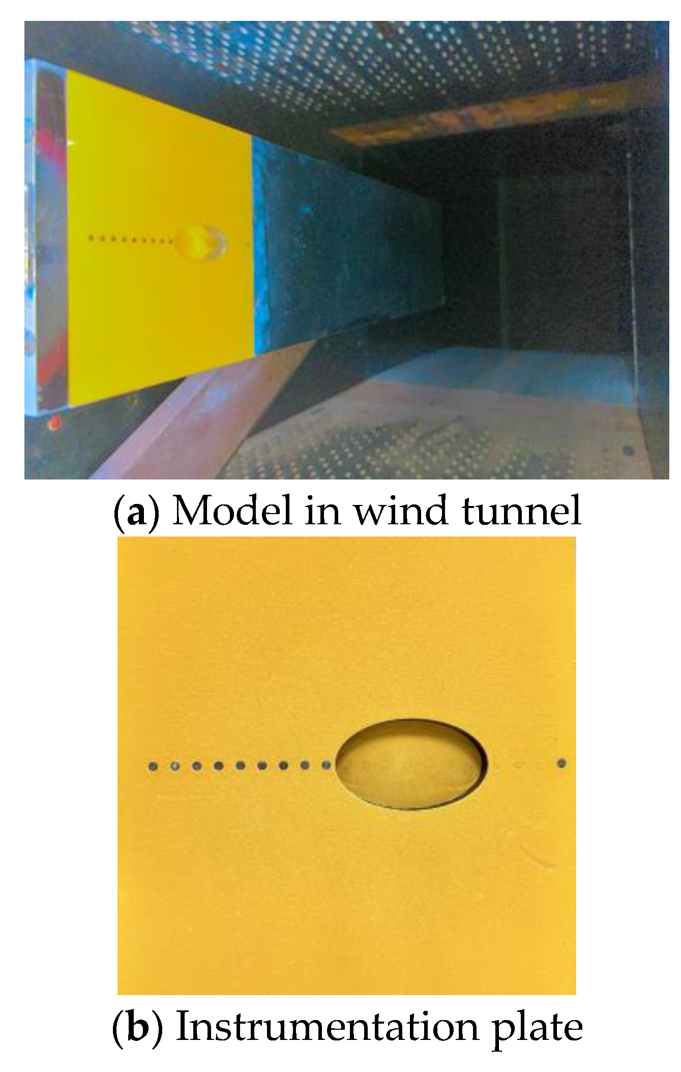
2.1. Transonic Wind Tunnel

The experiments were conducted in a blowdown-type wind tunnel at the Aerospace Science and Technology Research Center, National Cheng Kung University (ASTRC/NCKU). The dry high-pressure supply uses two compressors, two dryers and three storage tanks with a volume of 180 m³ with a maximum pressure of 50 bars. The dew point of high-pressure air flowing through the air dryers is maintained at −40 °C under normal operating conditions. Airflow from the supply tanks to the stagnation chamber is controlled by a sleeve rotating valve which continuously throttles the flow to maintain a specific stagnation pressure, p_o. A flow-conditioning module, comprising acoustic baffles, three screens and a honeycomb inside a stilling chamber, reduces noise and turbulence. A nozzle and two downstream choke flaps monitor the value of M. The operating Mach number ranges from 0.2 to 1.4, and the simulated Reynolds number is up to 20 million per meter. The square test section (600 × 600 mm² and 1500 mm in length) has perforated top/bottom walls and solid sidewalls. Downstream of the test section, a divergent subsonic diffuser decelerates the flow exiting to the atmosphere. The test conditions were recorded using a National Instruments system (Austin, TX, USA), including PXIe-8840 RT, PXI-7846, PXI-6511, and PXI-6513 NI-SCXI.

2.2. Models and Test Conditions

The test model was supported by a single sting mounted on the bottom floor of the test section. This comprised a flat plate (450 × 150 mm²) and an interchangeable instrumentation plate (170 × 150 mm²) with an elliptical cavity, as shown in Figure 1. Two side fences were also installed to prevent crossflow. Experimental conditions are shown in

Table 1. Experimental conditions.

M	po, Pa	Reδ	To
0.83	1.72 × 105	1.69 × 105	28–32 °C

. The boundary layer thickness for a naturally developed turbulent boundary layer, δ, was approximately 7 mm at a value of M of 0.83 [19]. The Reynolds number based on the boundary layer thickness, Re_δ, was 1.69 × 10⁵. The stagnation pressure was 172 ± 1 kPa, and the stagnation temperature was 28–32 °C. The values of ε for elliptical cavities were 0 (a cylindrical cavity), 0.66 and 0.87. The geometrical configurations of the cavities are listed in

Table 2. Cavity configuration.

L/H	L, mm	W, mm	ε
4.43	43
6.14	43	43.0, 32.3, 21.5	0, 0.66, 0.87
14.33	43
21.50	43

. The value of L (= 43 mm) is fixed, and W varies with the values of 43.0, 32.3 and 21.5 mm. The value of L/H ranges from 4.43 to 21.50 as the depth, H, varies from 2.0 to 9.7 mm.

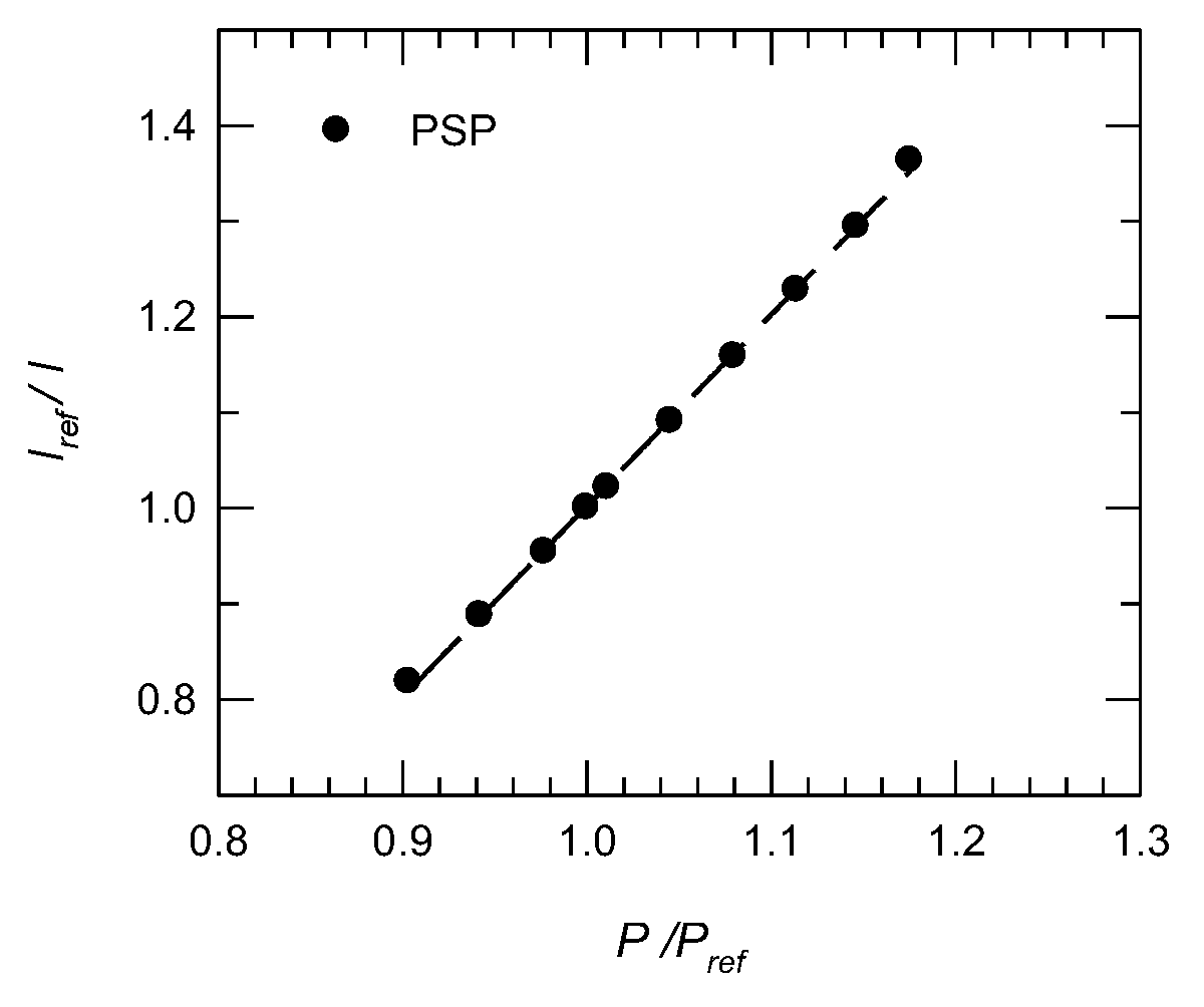
2.3. Pressure Measurements

Along the centerline of each instrumentation plate, there were 19 pressure taps (6 mm apart and 2.5 mm in diameter) drilled perpendicular to the test surface. All the pressure transducers (Kulite XCS-093-25A, B screen; Leonia, NJ, USA) were flush-mounted to the test surface for conventional discrete pressure measurements. Since there is low pressure sensitivity for these sensors, external amplifiers (Ectron Model 753A; San Diego, CA, USA) were used to improve the signal-to-noise ratio. The time-history outputs were recorded using a National Instruments system (NI-SCXI; Austin, TX, USA). The sampling rate was 5 μs, and there were 131,072 data points for each record. The uncertainty in the mean surface pressure coefficient, C_p (= (p_w − p_∞)/q), was 0.43%, where p_w and p_∞ are the mean and freestream pressures, respectively. The dynamic pressure is denoted as q.

Discrete pressure sensors provide a limited spatial resolution. PSP is a non-intrusive optical method that is used to visualize global surface pressure patterns [20,21,22,23]. If a light excites PSP, there is a transition for luminescent molecules to an excited state and to interact with oxygen molecules. Oxygen quenching represents the interaction between luminescent molecules and oxygen. The emission of molecules corresponds to energy transfers back to a ground state. The relationship between emission intensity and applied pressure is defined by the Stern–Volmer equation [24], where I_ref and P_ref are the respective reference intensities for the emission and the applied pressure. B represents pressure sensitivity, and A is a constant.

$$\frac{I_{ref}}{I}=A+B\left(\frac{P}{P_{ref}}\right)$$

(1)

For static calibration and wind tunnel tests, a base coating was sprayed onto the model surface using a spray gun (LVLP gun, DeVILBISS Demi1-0.8g; Scottsdale, AZ, USA). The PSP was a mixture of ruthenium (Ru(dpp)) and a polymer (RTV-118). The composition is listed in

Table 3. Composition of PSP.

Luminophore	Polymer	Solvent	Particle	Spray Area
Ru(dpp)	RTV-118	Toluene	SiO2	37.5 cm2
2.5 mg	250 mg	5 ml	125 mg

. Hollow SiO₂ mesoporous particles measuring 2 μm in diameter were added to the mixture to increase the oxygen permeability in the polymer binder and the PSP sensors. The respective absorption and emission spectra were measured at 411–467 nm and 597 nm. The PSP was illuminated using two light-emitting diode (LED) light sources (Revox SLG-55; Kanagawa, Japan). These light sources have a maximum brightness of 2100 lumens and a wavelength range of 300–800 nm. Two 550 nm low-pass filters were placed on the LEDs to filter incident light within the range of the luminescent signal wavelength. The emitted signal was captured using a 16-bit scientific Complementary Metal–Oxide Semiconductor camera (CMOS) (PCO. edge 3.1; Regensburg, Germany) with a 605 ± 15 nm high-pass optical filter to eliminate excitation light. The instrument has a resolution of 2048 × 1536 pixels and a pixel ≈0.3 mm. The sampling rate was set as 20 frames per second. The irreversible photo-degradation process proceeded at a rate of approximately 1% per hour.

There were 50 images recorded using the CMOS camera, and an averaged image was used for data reduction. The calibration curve is shown in Figure 2 and was determined using a reference image at P_ref and an applied pressure that varied from 0.9 to 1.18 bar. Uncertainty due to spatial non-uniformities in the emitted intensity, paint thickness and luminophore concentration was reduced using a ratio between images at P and P_ref (or wind-on and wind-off images from wind tunnel tests). The value of B was 0.64%/kPa, and the temperature sensitivity for PSP was −1.12%/°C.

Liu et al. [21] determined that aerodynamic forces deform the model, which leads to misalignment between the wind-on and wind-off images. This study used image registration to determine the pixel-to-pixel image ratio. Dark images were captured to remove pattern noise. A median filter function (a Matlab program) was used to remove shot noise and to preserve the pressure gradient at the edge in the acquired image. The CMOS camera recorded 50 images to reduce random noise for each wind tunnel test, and the acquired experimental results were considered time-averaged data. An in-house Matlab code was then used to transform the luminescent intensity into pressure data between the calibration and the experiment. Measurement uncertainty corresponded to cameras, light sources, test conditions and pressure/temperature sensitivity.

3. Results and Discussion

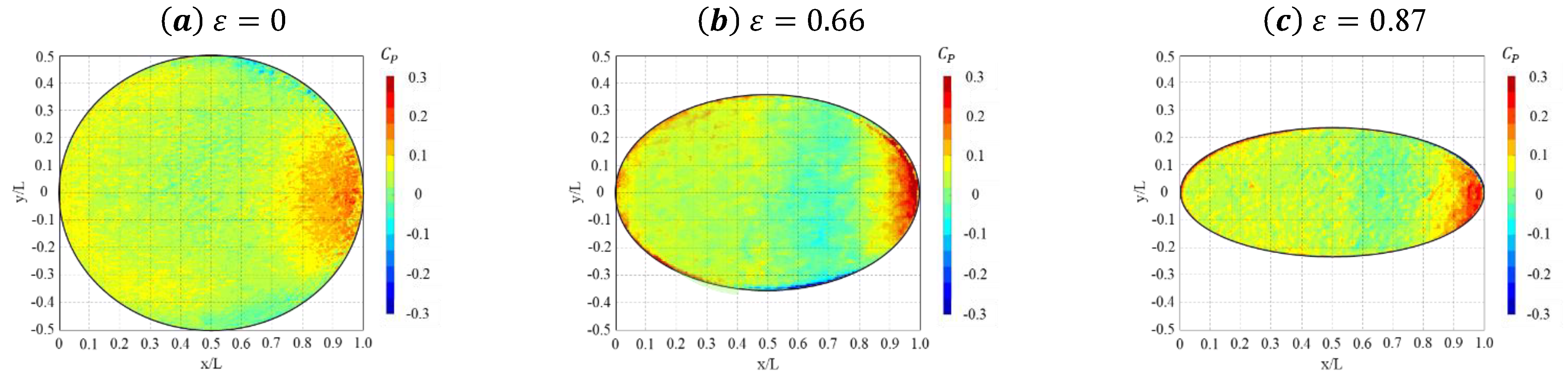
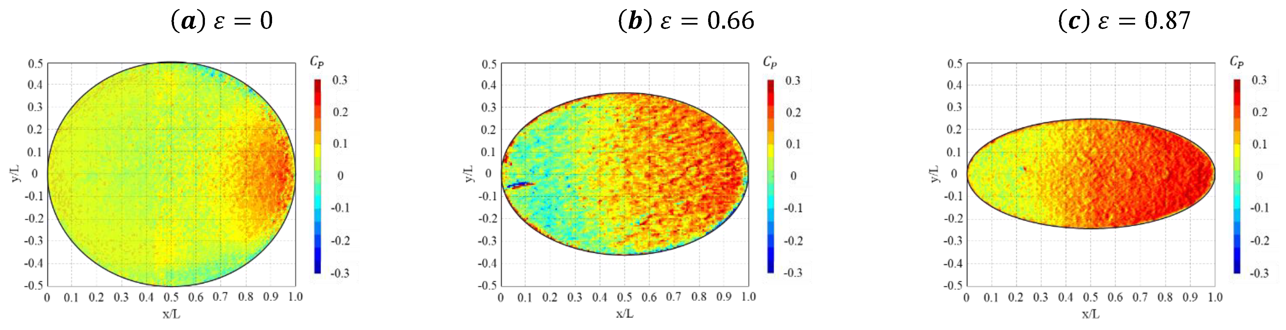
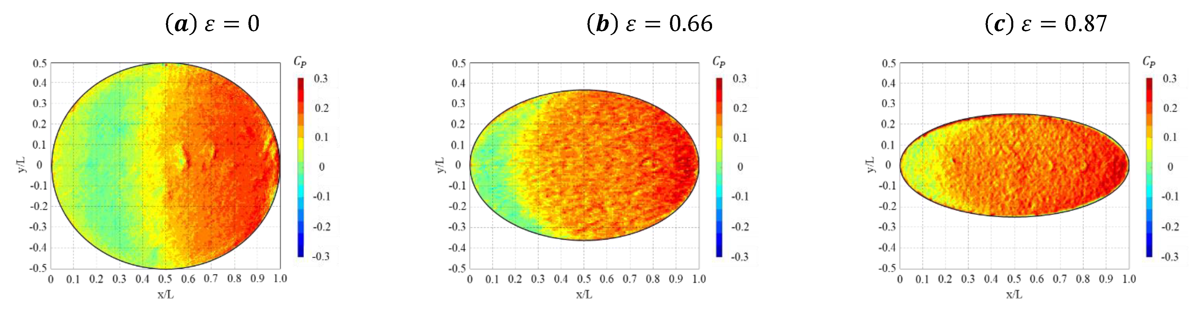
3.1. Global Pressure Pattern

The surface pressure pattern on the cavity floor for L/H = 4.43 is shown in Figure 3. The normalized x-coordinate (x^* = x/L) is in the streamwise direction. For ε = 0 (a cylindrical cavity, Figure 3a), there is a uniform pressure distribution until x^* ≈ 0.7, and an adverse pressure gradient occurs upstream of the rear face. This corresponds to a typical pressure distribution for an open-type cavity flow [5,6]. For ε = 0.66 (L/W = 1.33, Figure 3b) and 0.87 (L/W = 2.0, Figure 3c), there is a slight favorable pressure gradient until x^* ≈ 0.7–0.8, and the region in which C_p has a positive value is narrower. An arc-shaped pressure pattern near the rear face becomes more significant as ε increases because of the effect of the curvature of the rear wall. An increase in the value of C_p signifies greater inflow and outflow near the rear face as ε or L/W increases, which is similar to rectangular cavities [10].

For L/H = 6.14, the surface pressure pattern for ε = 0 is shown in Figure 4a, which represents a typical open-type cavity flow. There is a slight increase in the value of C_p downstream of the front edge in comparison with that for L/H = 4.43. For ε = 0.66 (Figure 4b), the region in which there is an adverse pressure gradient is expanded upstream, and the surface pressure pattern resembles a transitional–open cavity flow. This is also true for ε = 0.87 (Figure 4c). There is an open-type cylindrical cavity flow for L/H = 4.43−7.17 [14]. In this context, the boundary between different flow types varies for cylindrical and elliptical cavities.

As L/H increases, Figure 5a (14.33 and ε = 0) shows that the region in which C_p is positive moves upstream. The shear layer separates at the front edge and impinges on the cavity floor. This phenomenon becomes more significant as ε increases, as shown in Figure 5b (ε = 0.66) and Figure 5c (ε = 0.87). The surface pressure pattern is for a transitional–closed or closed cavity so that there is early transition from an open to a closed cavity flow as ε increases. For L/H = 21.50, Figure 6a shows a typical closed-type cylindrical cavity. The region in which C_p is positive moves further upstream, and an arc-shaped pressure pattern is shown in Figure 6b,c for ε = 0.66 and 0.87. Hering and Savory [15] demonstrated that there is an increase in entrainment over the sidewall for rectangular cavities with a greater value for L/W. For elliptical cavities, there is early shear layer impingement on the cavity floor as ε increases.

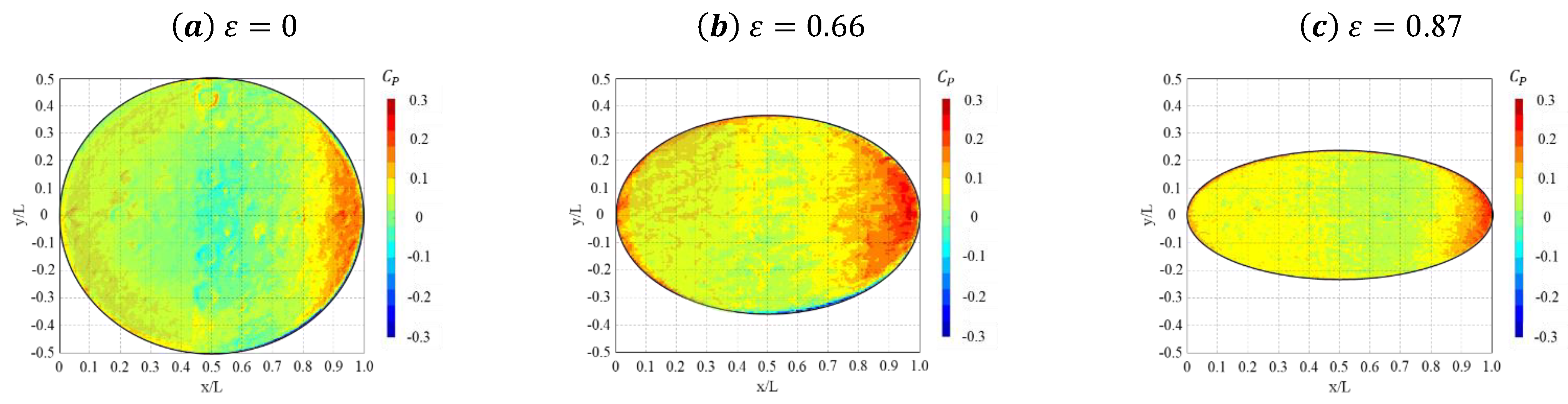
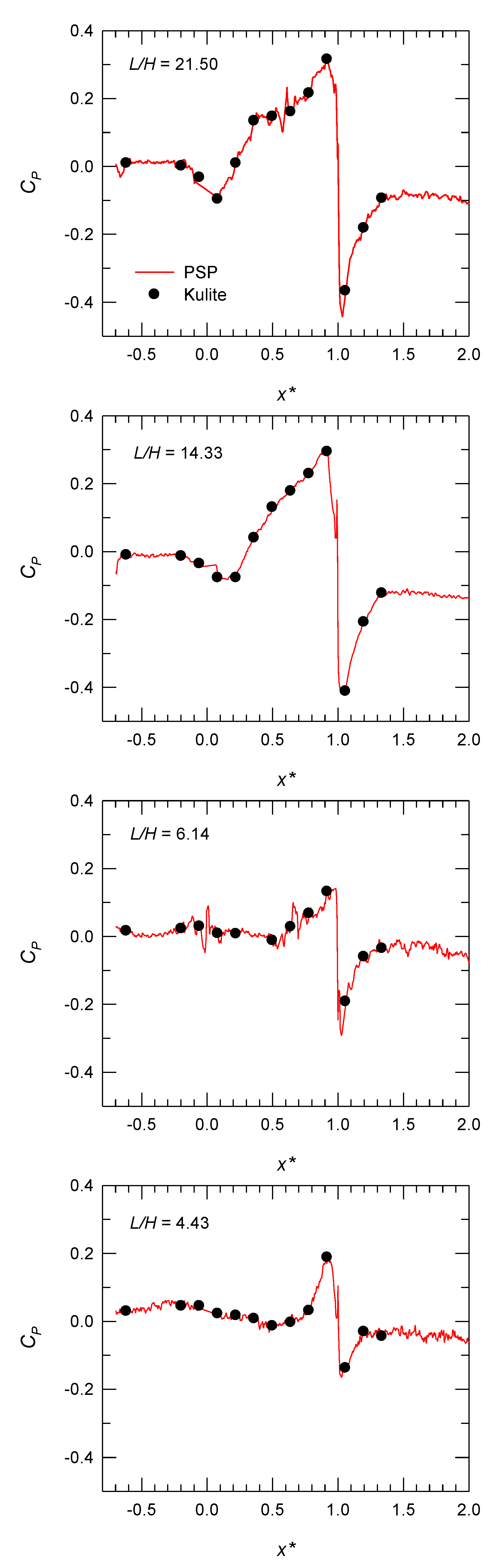
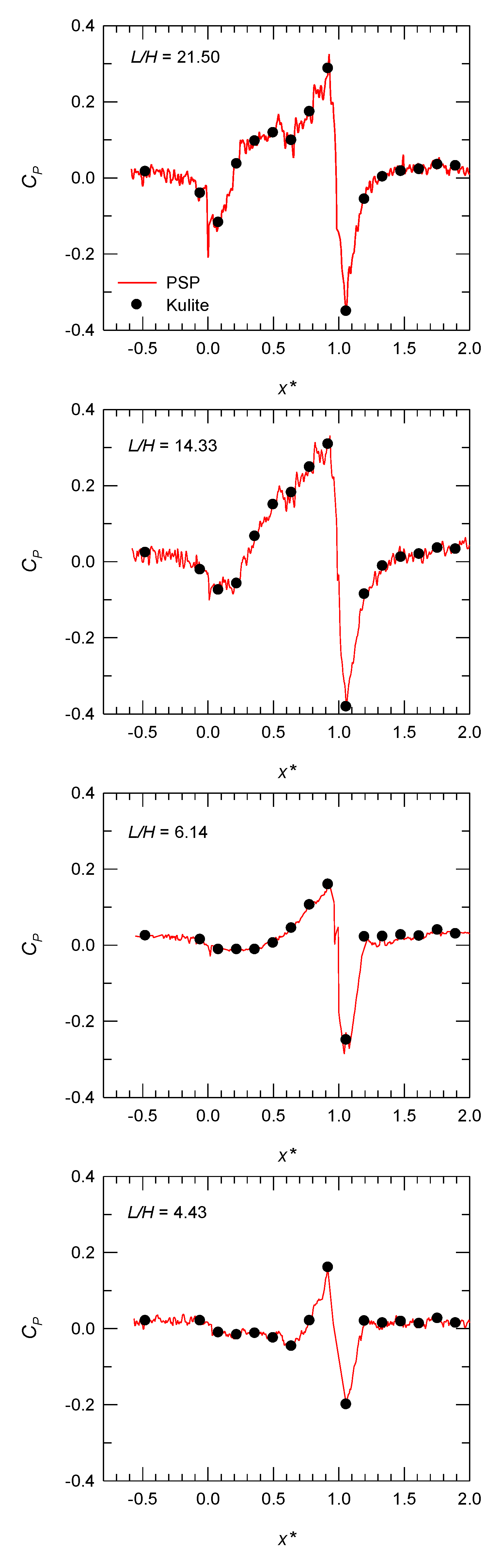
3.2. Mean Surface Distribution

The characteristics of a compressible cylindrical cavity flow were determined by Chung et al. using Kulite sensors [14]. There is an open-type cavity flow if D/H ≤ 6.14 and a transitional-type cavity for a D/H value of 8.60−21.00. Figure 7 shows the surface pressure distribution in the centerline (y^* = 0; ε = 0; L/H = 4.43–21.50), as measured using Kulite sensors and PSP. The two measurement techniques give comparable results. A greater deviation is observed near the rear edge. There is significant flow expansion near the front and rear edges for L/H = 14.33 and 21.50, and the respective peak pressure values, C_p,peak, at x^* = 0.92 are 0.29 and 0.31 as the value of L/H increases. There is a plateau (x^* = 0.37−0.46) in the C_p distribution for L/H = 21.50, which corresponds to a transitional–closed cavity. For L/H = 4.43 and 6.14, the static pressure distribution is uniform on the cavity floor, representing a typical open cavity flow, and rear-edge expansion is less significant than for L/H = 14.33 and 21.50.

For ε = 0.66 (L/W = 1.33), as shown in Figure 8, the surface pressure distribution is similar to that for ε = 0. There is a plateau at x^* = 0.36−0.78 for L/H = 21.50, so an increase in ε results in a lower value for a closed-type cavity. The value of C_p,peak at x^* = 0.92 is 0.28, which is slightly less than that for ε = 0. However, there is greater flow expansion near the rear edge because of an increase in the entrainment over the sidewall [15]. For L/H = 14.33, there is less expansion near the rear edge, and the value of C_p,peak at x^* ≈ 0.91 is 0.32. The flow resembles that for a transitional–closed cavity. For L/H = 6.14 and 4.43, the effect of ε is less significant. There is a decrease in the value of C_p,peak (= 0.19 and 0.14 for ε = 0.66 and 0.87, respectively) as ε increases. This is also true for L/H = 4.43. The surface pressure distribution for ε = 0.87 (L/W = 2.0), as shown in Figure 9, resembles that for ε = 0.66.

Near the rear edge, there is a circulation region for a closed cavity and a flapping motion in the shear layer for an open cavity. Figure 10 shows the coefficient for the difference in pressure near the rear face (the peak and the minimum), which is denoted as ΔC_p, corresponding to the flow mass exchange. For ε = 0, there is a slight variation in the value of ΔC_p for an open cavity (L/H ≤ 6.14). An increase in the value of L/H increases the value of ΔC_p, following a decrease for a transitional–closed cavity (L/H = 21.50). Flow expansion increases if there is an increase in the value of ε due to an increase in entrainment over the sidewall, particularly for L/H = 14.33 (a transitional cavity). This determines the effect of ε on flow development near the rear edge.

4. Conclusions

The presence of a cavity affects the surface pressure pattern inside and near the cavity. An open cavity flow is characterized by circulation in the cavity. An increase in the ratio between the cavity length and depth leads to a reduction in circulation and produces a transitional cavity flow. A closed-cavity flow features greater flow expansion at the front and rear edges. Previous studies mainly involved a rectangular cavity, not a cylindrical or elliptical cavity. The effect of wall curvature has not been determined.

This study determines the effect of the eccentricity of an elliptical cavity on the global surface pressure pattern at a freestream Mach number of 0.83 using pressure-sensitive paint. If the value for eccentricity (the ratio between the lengths of the major and minor axes) for an open cavity increases, the region in which there is an adverse pressure gradient expands upstream. A change in wall curvature affects flow expansion near the front and rear edges, and the boundary between different flow types varies. The flow characteristics of elliptical cavities depend on the ratio between the cavity length and depth, and the effect of eccentricity has a more significant effect on surface pressure distribution for a transitional–closed cavity.

References

1. Chen, H.; Zhong, Q.; Wang, X.K.; Li, D.X. Reynolds number dependence of flow past a shallow open cavity. Sci. China Technol. Sci. 2014, 57, 2161–2171. [Google Scholar] [CrossRef]
2. Zhang, C.; Li, R.F.; Xi, Z.J.; Wan, Z.H.; Sun, D.J. Effect of Mach number on the mode transition for supersonic cavity flows. Aerosp. Sci. Technol. 2020, 106, 106101. [Google Scholar] [CrossRef]
3. Chung, K.M.; Huang, Y.X.; Lee, K.H.; Chang, K.C. Reynolds number effect on a compressible cylindrical cavity flow. Chinese J. Aero. 2020, 33, 456–464. [Google Scholar] [CrossRef]
4. Oka, Y.; Ozawa, Y.; Nagata, T.; Asai, K.; Nonomura, T. Experimental investigation of the supersonic cavity by spectral-POD of high-sampling rate pressure-sensitive paint data. Exper. Fluids 2023, 64, 108. [Google Scholar] [CrossRef]
5. Charwat, A.F.; Roos, J.N.; Dewey, F.C.; Hitz, J.A. An investigation of separated Flows—Part I: The pressure field. J. Aerosp. Sci. 1961, 28, 457–470. [Google Scholar] [CrossRef]
6. Plentovich, E.; Stallings, R., Jr.; Tracy, M. Experimental cavity pressure measurements at subsonic and transonic speeds; NASA Technical Paper 3358; Langley Research Center, National Aeronautics and Space Administration: Hampton, Virginia, USA, 1993. [Google Scholar]
7. Chung, K.M. Characteristics of transonic rectangular cavity flows. J. Aircr. 2000, 37, 463–468. [Google Scholar] [CrossRef]
8. Rossiter, J. Wind tunnel experiments on the flow over rectangular cavities at subsonic and transonic speeds; Technical Report 64037; Royal Aircraft Establishment: Farnborough, UK, 1964. [Google Scholar]
9. Heller, H.; Bliss, D. Aerodynamically induced pressure oscillations in cavities physical mechanisms and suppression concepts; Technological Report AFFDL-TR-74-133; Air Force Flight Dynamics Laboratory: Wright-Patterson Air Force Base, OH, USA, 1975. [Google Scholar]
10. Chung, K.M. Three-dimensional effect on transonic rectangular cavity flows. Exper. Fluids 2001, 30, 531–536. [Google Scholar] [CrossRef]
11. Ozalp, C.; Pinarbasi, A.H.M.E.T.; Sahin, B. Experimental measurement of flow past cavities of different shapes. Exper. Thermal Fluid Sci. 2010, 34, 505–515. [Google Scholar] [CrossRef]
12. Verdugo, F.R.; Guitton, A.; Camussi, R. Experimental investigation of a cylindrical cavity in a low Mach number flow. J Fluids Structures 2012, 28, 1–19. [Google Scholar] [CrossRef]
13. McCarthy, P.W.; Ekmekci, A. Flow features of shallow cylindrical cavities subject to grazing flow. Phys. Fluids 2022, 34, 027115. [Google Scholar] [CrossRef]
14. Chung, K.M.; Lee, K.H.; Chang, K.C. Characteristics of cylindrical cavities in a compressible turbulent flow. Aerosp. Sci. Technol. 2017, 66, 160–164. [Google Scholar] [CrossRef]
15. Khadivi, T.; Savory, E. Experimental and numerical study of flow structures associated with low aspect ratio elliptical cavities. J. Fluids Eng. 2013, 135, 041104-1. [Google Scholar] [CrossRef]
16. Hering, T.; Savory, E. Flow regimes and drag characteristics of yawed elliptical cavities with varying depth. J. Fluids Eng. 2007, 129, 1577–1583. [Google Scholar] [CrossRef]
17. Khadivi, T.; Savory, E. Effect of yaw angle on the flow structure of low aspect ratio elliptical cavities. J. Aerosp. Eng. 2017, 30, 04017002. [Google Scholar] [CrossRef]
18. Guo, G.; Qin, L.; Wu, J. On aerodynamic characteristics of rarefied hypersonic flows over variable eccentricity elliptical cavities. Aerosp. Sci. Technol. 2023, 134, 108160. [Google Scholar] [CrossRef]
19. Chung, P.H.; Huang, Y.X.; Chung, K.M.; Huang, C.Y.; Isaev, S.A. Effective distance for vortex generators in high subsonic flows. Aerosp. 2023, 10, 369. [Google Scholar] [CrossRef]
20. Liu, T.; Campbell, B.T.; Burns, S.P.; Sullivan, J.P. Temperature-and pressure-sensitive luminescent paints in aerodynamics. Appl. Mech. Rev. 1997, 50, 227–246. [Google Scholar] [CrossRef]
21. Liu, T.; Guille, M.; Sullivan, J.P. Accuracy of pressure-sensitive paint. AIAA J. 2001, 39, 103–112. [Google Scholar] [CrossRef]
22. Zare-Behtash, H.; Yang, L.; Gongora-Orozco, N.; Kontis, K.; Jones, A. Anodized aluminium pressure sensitive paint: Effect of paint application technique. Meas. 2012, 45, 1902–1905. [Google Scholar] [CrossRef]
23. Kasai, M.; Suzuki, A.; Egami, Y.; Nonomura, T.; Asai, K. A platinum-based fast-response pressure-sensitive paint containing hydrophobic titanium dioxide. Sensors Actr. A-Phys. 2023, 350, 114140. [Google Scholar] [CrossRef]
24. Bell, J.H.; Schairer, E.T.; Hand, L.A.; Mehta, R.D. Surface pressure measurements using luminescent coatings. Annul. Rev. Fluid Mech. 2001, 33, 155–206. [Google Scholar] [CrossRef]
Figure 1. Model setup.
Aerospace 11 00159 g001
Figure 2. Calibration curve for PSP.
Aerospace 11 00159 g002
Figure 3. Surface pressure distribution for a cavity with L/H = 4.43.
Aerospace 11 00159 g003
Figure 4. Surface pressure distribution for a cavity with L/H = 6.14.
Aerospace 11 00159 g004
Figure 5. Surface pressure distribution for a cavity with L/H = 14.33.
Aerospace 11 00159 g005
Figure 6. Surface pressure distribution for a cavity with L/H = 21.50.
Aerospace 11 00159 g006
Figure 7. Mean surface pressure distribution for ε = 0 (red solid line: PSP data; black points: Kulite data).
Aerospace 11 00159 g007
Figure 8. Mean surface pressure distribution for ε = 0.66 (red solid line: PSP data; black points: Kulite data).
Aerospace 11 00159 g008
Figure 9. Mean surface pressure distribution for ε = 0.87 (red solid line: PSP data; black points: Kulite data).
Aerospace 11 00159 g009
Figure 10. The effect of eccentricity on rear-edge expansion.
Aerospace 11 00159 g010