1. Introduction
Dirigibles, or airships, present a unique operational advantage by combining energy-efficient cruising, a distinctive characteristic of fixed-wing aircraft, with the capability to hover, which is present in rotary-wing vehicles [
1]. Even the best hybrid VTOL aircraft fail to hover efficiently due to the energy needed to counteract the gravitational force, which, in airships, is granted by the buoyancy gas. They are also safer than other platforms if failure or degradation occurs, as they descend slowly to the ground in such cases. The combination of these features with the notable evolution in aerial robotics in the last 20 years has led to a resurgence in interest in the development of airship applications like cargo transportation [
2], telecommunications [
3] and environmental monitoring [
4].
This last theme is the focus of this work, in the context of the national project InSAC
https://insac.eesc.usp.br/ (accessed on 15 February 2024). The project aims to develop a semi-autonomous airship capable of cruise flight and ground-hover for environmental monitoring/surveillance tasks in the Amazon rainforest.
Usually, these two flight modes (cruise/hover) encompass two conflicting flight mission objectives: total mission area coverage vs. detailed data acquisition. Considering the aircraft autonomy and the amount of time needed to acquire a given unit of data, cruising is associated with minimizing the total mission time per unit of data, allowing for the coverage of a larger area. Hovering flight, instead, seeks to maximize the amount of data acquired in a specific location.
However, in both cases, robust flight under actual weather conditions is still one of the biggest issues that prevent airships from fully realizing maneuverability advantages. In this way, safe and accurate airship control under strong wind conditions is still an open theme of research investigations due to the limited lateral actuation available in the vehicle [
3,
5].
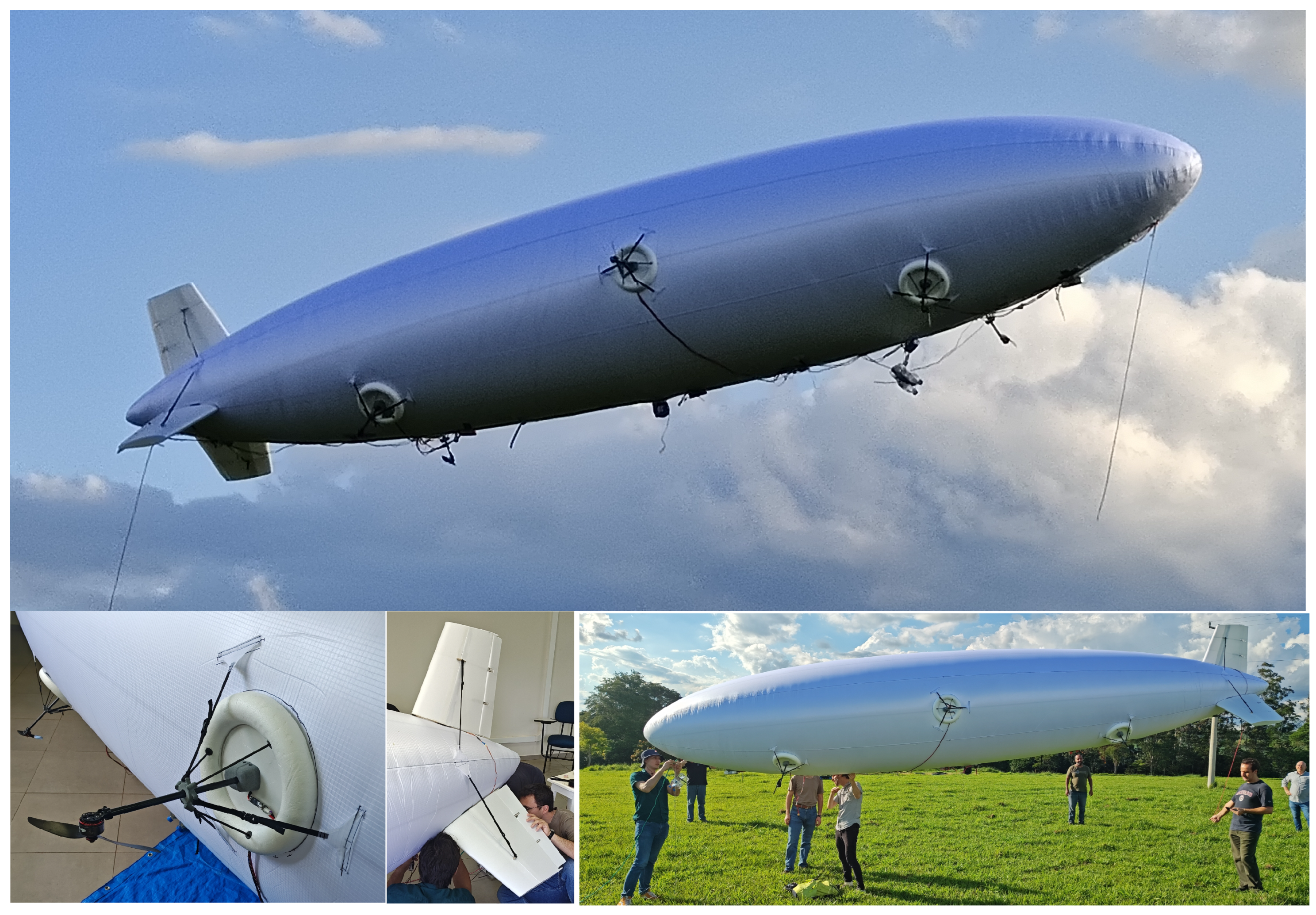
The proposal of an airship design with increased maneuvering capability is the first contribution of this work. Here, we present the design and application of a new kind of six-propeller electrical airship with improved actuation features (
Figure 1). The airship prototype, named Noamini, is tailored for a specific class of semi-autonomous airships designed for environmental monitoring, a context where large area coverage and the quantity of acquired data are equally important.
The blimp, built in Germany, has an important innovation: an actuation system with six electric motors with independent tilting propellers (up to 360 deg), allowing the craft to take off and land vertically, perform faster yaw/pitch maneuvers and improve its hover controllability in the presence of wind. The vehicle can be used in two-, four- or six-motor configurations, depending on the mission to be executed. It also enables the use of differential propulsion in front/rear, left/right or cross configurations, improving the control torque to compensate for wind disturbances at low airspeeds, where the tail efficiency fails.
Further, we developed a high-fidelity airship simulator for the Noamini airship, whose aerodynamic model is adapted from the seminal work of [
6], making use of a large wind tunnel database. The airship simulator in Simulink/Matlab also includes the modeling of sensors/actuators, derivative filters and wind estimators [
7]. The simulator environment was used to test and validate a control/guidance approach derived for the path-tracking task of the Noamini airship.
The design of automatic pilots for autonomous airships is known to be a great challenge, as these vehicles are usually underactuated, with coupled nonlinear underdamped dynamics [
8]. Furthermore, many existing nonlinear control approaches, such as sliding mode [
9], backstepping [
10] and Dynamic Inversion [
11], are not sufficiently robust, requiring an accurate knowledge of the vehicle model [
12].
In this work, we apply the Incremental Nonlinear Dynamic Inversion (INDI) approach, developed in 2010, which is a natural evolution of the classic Nonlinear Dynamic Inversion (NDI). Aiming to reduce the model dependency of classic controllers, INDI assumes that the change in control is significantly faster than the change in the state, such that the sensor feedback supplies the necessary information about the model to the controller, which is thus considered a “sensor-based” controller [
12], instead of a “model-based” one. Due to its robustness properties, INDI control has been successfully applied to a number of different aerial vehicles since then, including an e-VTOL aircraft from NASA Ames [
13], a Passenger Aircraft from DLR [
14] and conventional drones [
15,
16,
17,
18].
For the guidance approach, we implemented L1 guidance, an advanced path-following algorithm that extends the functionality of traditional autopilots through the inclusion of a virtual target that moves along the path, tracked by the vehicle’s attitude control effectors [
19].
In this way, the second contribution of this paper is the design and testing of a control/guidance approach for the waypoint-tracking mission of the six-propeller airship.
The remainder of this paper is organized as follows.
Section 2 describes the vehicle application scenario: the surveillance and environmental monitoring of forest segments in the Amazon rainforest region.
Section 3 describes the Noamini platform and its subsystems.
Section 4 summarizes the vehicle modeling and simulator.
Section 5 presents the proposed guidance and control approach for the waypoint-tracking problem.
Section 6 presents the simulation results for a typical waypoint-tracking mission, and
Section 7 concludes the paper.
2. Forest Surveillance and Environmental Monitoring
The Amazon biome is immensely rich and of recognized ecological relevance [
20]. The Amazon rainforest is dense, flooded by the Amazon river and its tributaries, forming the world’s larger river basin, with a total area at the same scale of the largest countries, and it is sparsely occupied by humans. Therefore, the protection of the ecosystem, the conservation and sustainable use of natural resources, and the sustainable development of existing population centers pose complex challenges that are beyond the capability of any current technology. In this work, the authors are interested in two different missions: aerial surveillance and environmental monitoring.
2.1. Aerial Surveillance
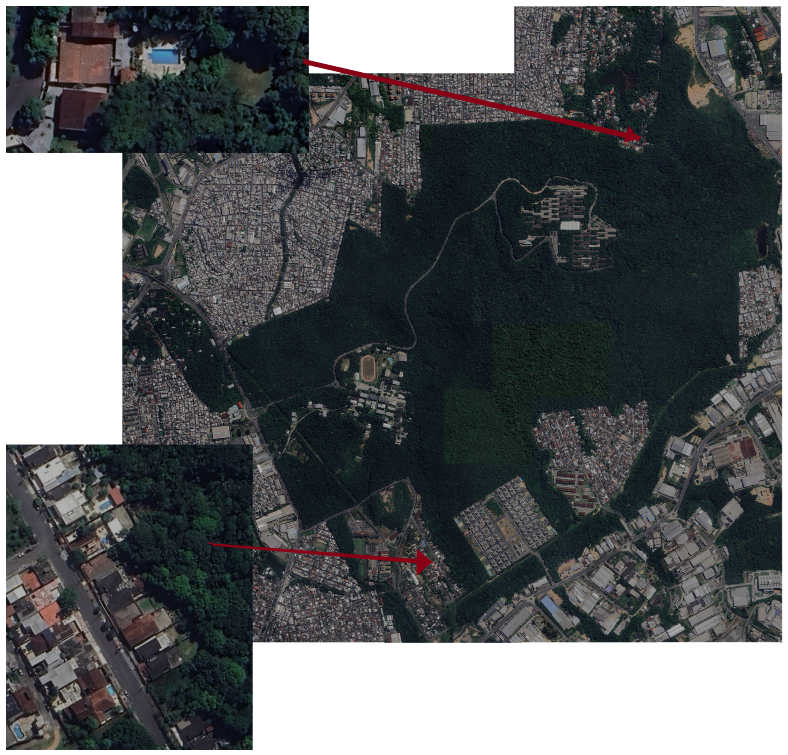
For aerial surveillance, we are interested in a specific, although crucial, aspect of Amazon forest conservation: the interaction between urban areas and the surrounding forest. The inevitable anthropogenic pressure promotes deforestation by extending urban occupation toward the forest. Consider, for instance, the native forest segment where the campus of the Federal University of Amazon is located (
Figure 2). This 6,700,000 m
2 protected reserve is the world’s third largest native forest segment in an urban area. Despite being protected by both state and federal laws, for decades, residents have enlarged their properties toward the forest.
Figure 2 presents two examples (among many others) of such occurrences, indicated by red arrows. Furthermore, we can clearly see the value of low-altitude data over high-altitude images to detect these events in a timely manner.
Currently, a significant portion of information available about the forest comes from satellite images provided at intervals of days or even weeks [
21]. Even when considering the importance of these data, they are less effective for short-term actions, such as activating the response to a wildfire before it escalates. In those contexts, the application of low-altitude aerial monitoring systems brings indisputable advantages by providing multimodal information with high regularity (time between samples), small granularity (order of magnitude of the sampling unit) and low latency (time between acquisition and availability of the sample) [
22].
The surveillance mission profile combines a flyover with hovering at specific points of interest. The typical zig-zag scan flight for area coverage is not suitable here, as the conflicting areas are on the forest border, and fixed-wing aircraft would require more than one pass over a suspected location or an off-line inspection of the acquired imagery data to search for anomalies (irregular deforestation) [
21]. On the other hand, one may realize that, even considering an urban segment, this reserve is too large for hover-capable rotary-wing aircraft. Only airships can combine cruise flight mode with hovering to go through the reserve border and focus on points of interests, whenever necessary [
4]. Moreover, the airship has the capability to modulate the hovering altitude according to the situation, and, as a bonus, it can zig-zag in an area if scanning is necessary.
2.2. Environmental Monitoring
The environmental monitoring missions concern the gathering of multimodal sensory data. The payload includes images in multiple spectral ranges, lidar data, and air chemical and physical parameters. There are three mission objectives identified so far:
The analysis of the aerosol layer above the canopy. This layer is of great research importance, as the rainforest is known for having a thick aerosol layer, the droplets of which capture all sorts of suspended particles. Airships are the only aerial vehicle capable of sensing the aerosol composition and density. Rotary wings disperse the droplets, and the turbulence of fixed-wing aircraft reduces the correlation between the acquired data and the actual layer [
23];
Forest inventory. The native segment is a valid representation of the Amazon forest. Researchers are interested in mapping the species of trees, tracking their changes during the year and even producing forecasts for those with economic value. An airship with cruise flight capability is of use in this case [
24,
25];
Wildlife monitoring. Forest areas close to human occupation are known to have a severe depletion in wildlife diversity. Moreover, street dogs and cats act as invasive species, decimating small animals, such as wild rodents and birds. Once more, an airship is a very suitable monitoring platform due to its capacity to quietly fly over an area of interest and stay above a point of interest [
4].
The payload details are not yet available, but the authors are very confident that Noamini will be able to perform a diverse variety of missions simultaneously.
3. Airship Platform
The Noamini prototype is described in this section, together with its sensor set and actuators, yielding an overview of the vehicle design and operation, including its configurations and limitations.
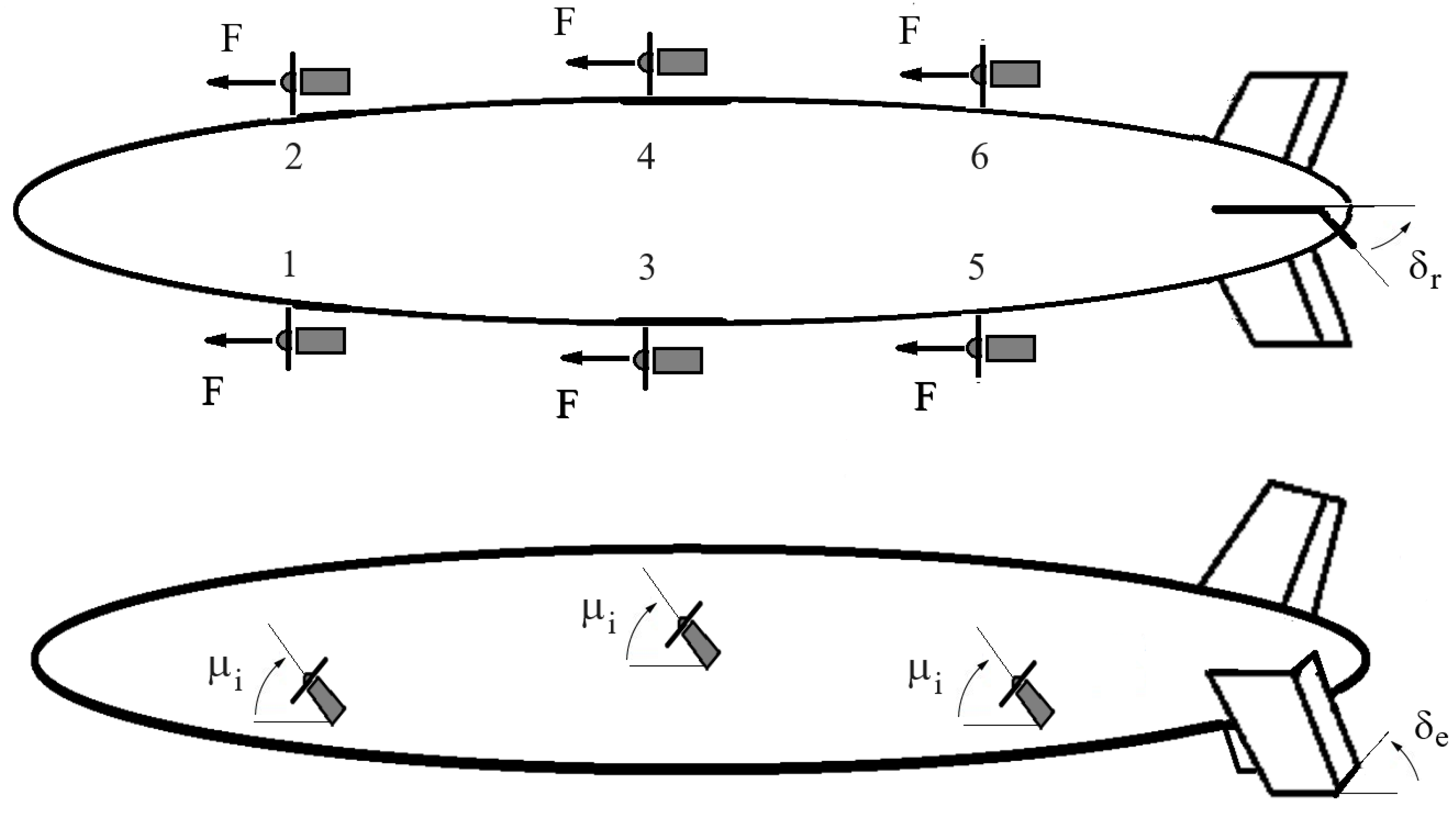
The primary actuators within the Noamini airship (refer to
Figure 3) consist of three aerodynamic tail fins in an inverted-Y configuration, working as a rudder, an elevator and an aileron, and six tilting electric thrusters. These thrusters serve the dual purpose of compensating for the aircraft’s excess weight during low-speed operation (e.g., hovering) and enhancing maneuverability across the entire flight profile. The airship is equipped with a ballonet to allow altitudes up to 200 m to be reached while maintaining the envelope pressure.
The vector of control inputs, , is composed of the commands of the elevator, aileron and rudder (, , and ), plus the six inputs representing the normalized input voltages of the i-th thruster, and the tilting angles of the i-th propeller, given by ….
Taking advantage of the motors’ differential action while reducing the redundancy, the propellers’ power can be configured in different forms: all with the same forward power , left/right differential , front/back differential , and cross-differential . Similar configurations can be used for the propeller tilting angles ().
4. Airship Model and Simulator
A successful control design relies on a good comprehension of the airship model and behavior, along with the use of a reliable simulator. This section summarizes the results presented in [
11], adapted to the new six-propeller vehicle. The reader should refer to [
11] for more details.
4.1. Airship Dynamic Model
The dynamic model is a mathematical description of the airship motion, representing the connections between the control inputs and the state variables [
26], that is,
with the variables defined as follows:
The state includes the linear and angular inertial velocities of the airship expressed in the body-fixed frame, the Cartesian position of its center of volume in the inertial frame, and the attitude of the airship, given by the Euler angles .
The input vector , where , and are described above.
The disturbance vector encompasses the wind entry denoted by a constant wind velocity in the inertial frame, along with a six-component stochastic vector that models atmospheric turbulence. It is expressed by the linear wind velocity and the angular wind velocity .
Here, we should remark on a set of important assumptions and considerations regarding the development of the airship model [
11], as stated below:
As a light vehicle that displaces a large volume of air, which is of the same order of magnitude as its mass, the airship’s virtual (added) mass and inertial properties become significant. In other words, the lighter-than-air vehicle behaves as if it has mass and inertia greater than those given by the simple sum of its mass/inertia components.
Three types of mass and inertia matrices are assumed: the mass and inertia (
of the vehicle itself; the mass and inertia (
of the buoyancy air, corresponding to the mass of displaced air that could fill exactly the ellipsoidal volume of the envelope, with its associated inertia moment
; and the virtual mass and inertia (
, which can be understood as the surrounding air mass displaced by the airship during its relative motion in the air. For more details on these different types of masses and inertias of lighter-than-air vehicles, the reader should refer to [
11].
The airship mass may vary in the flight due to the inflation or deflation of the air ballonet.
The aeroelastic effects are neglected, as the airship is assumed to be a rigid body.
The differential equation describing the airship movement is obtained from the second Newton Law applied to the vehicle inertial velocities given in the local frame. If we represent these linear and angular velocities as
, then the dynamic equation can be derived as follows [
26]:
where
represents the
mass matrix, encompassing both real and virtual inertia elements characteristic of the dynamics of floating air vehicles. The
vectors given by
,
,
,
and
relate, respectively, to the inertial, aerodynamic, propulsive, gravitational/buoyancy and wind-induced forces and moments.
4.2. Airship Dynamic Simulator
The dynamic model derived above encompasses 6 degrees of freedom and serves as the foundation for a MATLAB/Simulink simulator, facilitating the project, test and validation of the control and guidance approaches [
26].
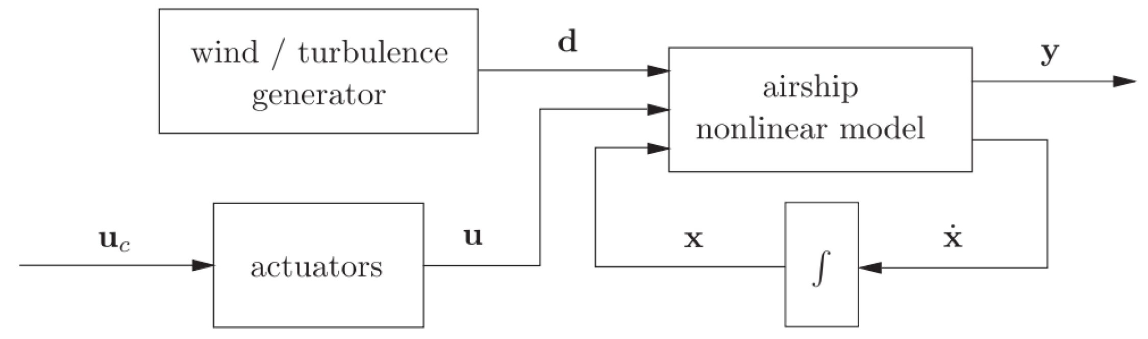
The block diagram describing the airship simulator framework is given in
Figure 4 below.
The dynamics of the airship, as outlined in Equation (
1), depend on the state variables (
), the inputs from the actuators (
) and the wind disturbances (
), whose stochastic component comes from a Dryden model with three white noise inputs [
27]. The model of the actuators includes the propeller and tail surface dynamics with delays and level/rate limits. The output vector
corresponds to the monitored signals, available through the sensors, which are modeled to include noise, bias, saturation and quantification [
7]. Further, some signals, like the attitude angles, are not directly measured, requiring state observers that are included in the simulator, together with a Kalman Filter for wind estimation [
7].
The aerodynamic model relies on the groundbreaking research introduced by [
6,
28] and utilizes data from a wind tunnel database built for the modeling of the Westinghouse YEZ-2A airship. The aerodynamic coefficients on this dataset depend on the aerodynamic incidence angles (
and the deflections of the tail surfaces
,
,
. The aerodynamic incidence angles, originally limited to ±30 degrees, were further extended to cope with the usual range of angles of attack in a common flight, using curve-fitting and extrapolation procedures [
26].
Additional features of the Noamini airship simulator are as follows:
The inclusion of models of the motors and propellers, as well as the discharge model of the batteries (three packs, one for one pair of motors).
The inclusion of a nonlinear-based optimization routine to find the trim conditions and linearized models, which can be computed for different propulsion modes.
Finally, the six propellers result in redundant propulsion, and we assume that each of them may be controlled both in the throttle command and the vectoring angle. With this redundancy, it may be possible to choose among active propellers, minimizing a given cost function.
4.3. Linearized Longitudinal/Lateral Dynamics
The airship dynamics, which are highly nonlinear, vary significantly with the operational condition. As the airspeed varies from hovering flight (HF) to cruise or aerodynamic flight (AF), different actuators are used, yielding different behaviors for the vehicle [
7,
11]. In this way, the complexity of this nonlinear model justifies the derivation of a simplified linearized version, which is also useful for the design of the incremental controller (INDI).
The linearization of the model is performed around an equilibrium point, meaning a given operating condition, like horizontal flight, at a fixed airspeed and altitude [
7,
11]. As a consequence of the linearization process, a decoupled vehicle description is derived, with two independent movements: longitudinal motion (in the vertical plane) and lateral motion (in the horizontal plane plus rolling).
The longitudinal (
v) and lateral (
h) models are represented by the following:
The state vector corresponds to small variations in the longitudinal velocity, vertical velocity, pitch rate, pitch angle and altitude. The input represents the variations in elevator deflection, total thrust, forward differential thrust and the synchronized vectoring angle, respectively.
The state vector corresponds to small variations in the sideslip angle, roll rate, yaw rate, roll angle and yaw angle, respectively. The input includes, respectively, the variations in aileron and rudder deflections, left/right differential thrust, cross-differential thrust and the left/right differential tilting angle.
5. Control and Guidance Proposal
In the search for airship autonomy, it is fundamental to assure good positioning and path-tracking features for the control and guidance (CG) framework. In our case, the proposed architecture for the CG system encompasses four components: path planning, guidance, control and data acquisition [
5,
7]. The path planner generates the trajectory reference for the guidance loop, which tries to minimize the pose (position/orientation) error, while the control level tracks the velocity and acceleration commands. The data acquisition block is composed of data sensing, filtering and estimation and is used to acquire the filtered signals used by the other components [
7]. This modularization allows the guidance strategy to switched for different mission tasks while maintaining the stability/performance of the control loop. Also, tuning is easier once the tests can be conducted with a modular procedure.
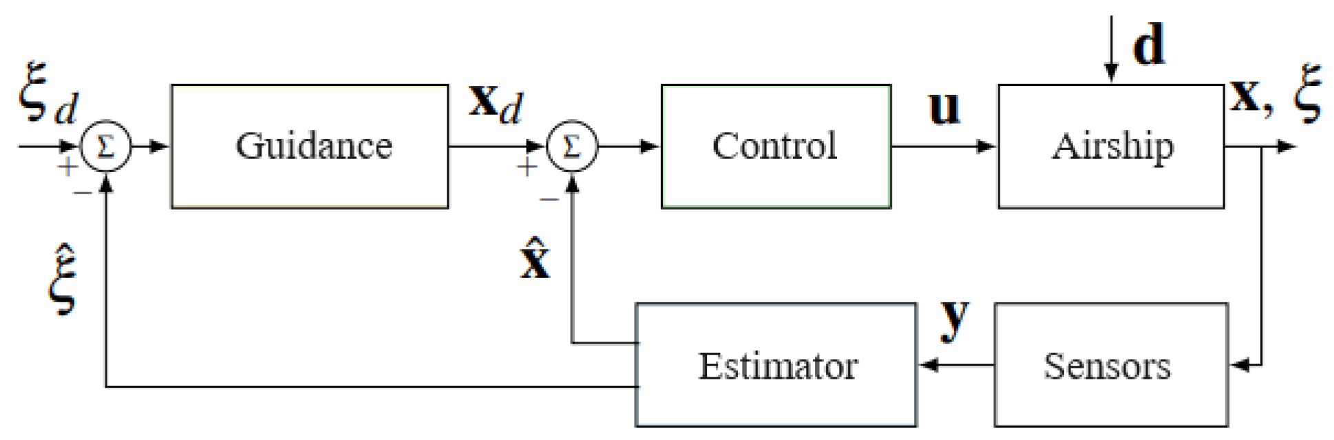
Figure 5 shows a block diagram with the proposed overall navigation architecture, where
is the vector of linear/angular velocities, and
is the actual airship position vector, both in the global frame, with
as the desired position. Further,
is the airship control input, and
is the wind/gust disturbance vector.
Prior to presenting the control/guidance approaches, it is important to remark on the challenges related to the control of this type of hexa-propeller lighter-than-air vehicle.
Firstly, we have to consider the issue of the actuator efficiency, which is heavily dependent on the airship flight region.
In the low-airspeed scenario (HF), the tail has reduced effectiveness, as the control forces generated by the surface deflections depend on the air-relative velocity. In this condition, the airship is mainly controlled by the force inputs coming from the six propellers, which provide longitudinal and vertical forces, through the tilting angle vectorization [
7,
11].
As opposed to this, in aerodynamic flight (AF), the tilting angles of the propellers are no longer necessary to compensate for the excess of weight, and the moment generation is easily implemented by the tail fins. In this case, the surface deflections of the inverted “Y” correspond to the three regular inputs of the aileron, elevator and rudder, which generate the roll, pitch and yaw moments.
Another important point is that, although 15 control inputs are presented (see the components of vector ) to control six forces (three forces and three torques), the airship still presents numerous limitations for the control design of the full flight envelope, among which we can state the following:
The majority of the actuators indeed act on the longitudinal motion.
No direct actuator is available to generate lateral-side forces on the airship (.
Although independent vectoring angles for the six engines are possible, it is safe and practical to consider all of them with the same vectoring angle, except, eventually, for the front/back differential case in the lower four-motor configuration.
As the tail surfaces’ actuation depends on the air velocity, their effectiveness is reduced at low airspeeds, when the airship is controlled mainly by the propeller thrust.
All the actuators have level saturation and rate limits that need to be taken into account while not forgetting about the response time of the engines as well.
All these aspects greatly increase the complexity of the design of the airship control/guidance system, as described below.
5.1. Incremental Nonlinear Dynamic Inversion Control (INDI)
In the last 20 years, different airship control approaches have been proposed, like sliding mode (SMC) [
9], backstepping [
10], Dynamic Inversion, gain scheduling [
11] and backstepping SMC [
26]. However, in the last decade, a new approach has gained the attention of control engineers in this field, that is, Incremental Nonlinear Dynamic Inversion (INDI) [
7,
29].
INDI was a natural evolution of one of the most known nonlinear control methods—Nonlinear Dynamic Inversion (NDI), or “feedback linearization”, which uses nonlinear feedback to cancel out the plant nonlinearities. A serious drawback of the NDI-based control law, which motivated the development of INDI, is that the precise modeling of nonlinear plant dynamics is necessary for a
direct model cancellation, making it a non-robust approach [
12].
In this way, the incremental version of NDI, known as INDI, was presented in 2010 to attack the robustness problem by reducing the model dependency through the use of fast sensor measurements [
30]. Following the INDI concept, firstly, the model to be inverted is written in an incremental form, and, with the use of a Taylor series, the incremental control input is derived [
31]. To reduce the model dependency, INDI assumes that the change in the control signal is much faster than the change in the state, which is known as the “time scale separation” [
12]. In this way, the sensor feedback supplies the necessary information about the model for INDI, which is thus considered a “sensor-based” controller [
12]. Due to its robustness properties, INDI control has been successfully applied to a number of different aerial vehicles since then, including an e-VTOL aircraft from NASA Ames [
13], a Passenger Aircraft from DLR [
14] and conventional drones [
16,
17,
18].
The basic formulation of Incremental Dynamic Inversion is as follows. Consider the nonlinear plant dynamics, assumed to be affine in the input:
where
is the state vector, and
is the control input.
Instead of inverting the full dynamics like in NDI, INDI linearizes and inverts the system dynamics at the previous state and previous input .
In this way, if we apply a Taylor series expansion to the plant Equation (
5), and if we neglect the higher-order terms, we have
Further, if we use a sufficiently fast sampling time on the flight control computer, we can assume that the state changes are negligible (
). This assumption only holds when using sufficiently fast actuators, such that their effects over the dynamics is more important than the changes in the state vector [
31].
Hence, Equation (
6) can be simplified to
And the INDI control law is thus derived as
To confirm the correctness of the design, we substitute this control law into the linearized system dynamics to obtain
where
denotes the desired commanded reference
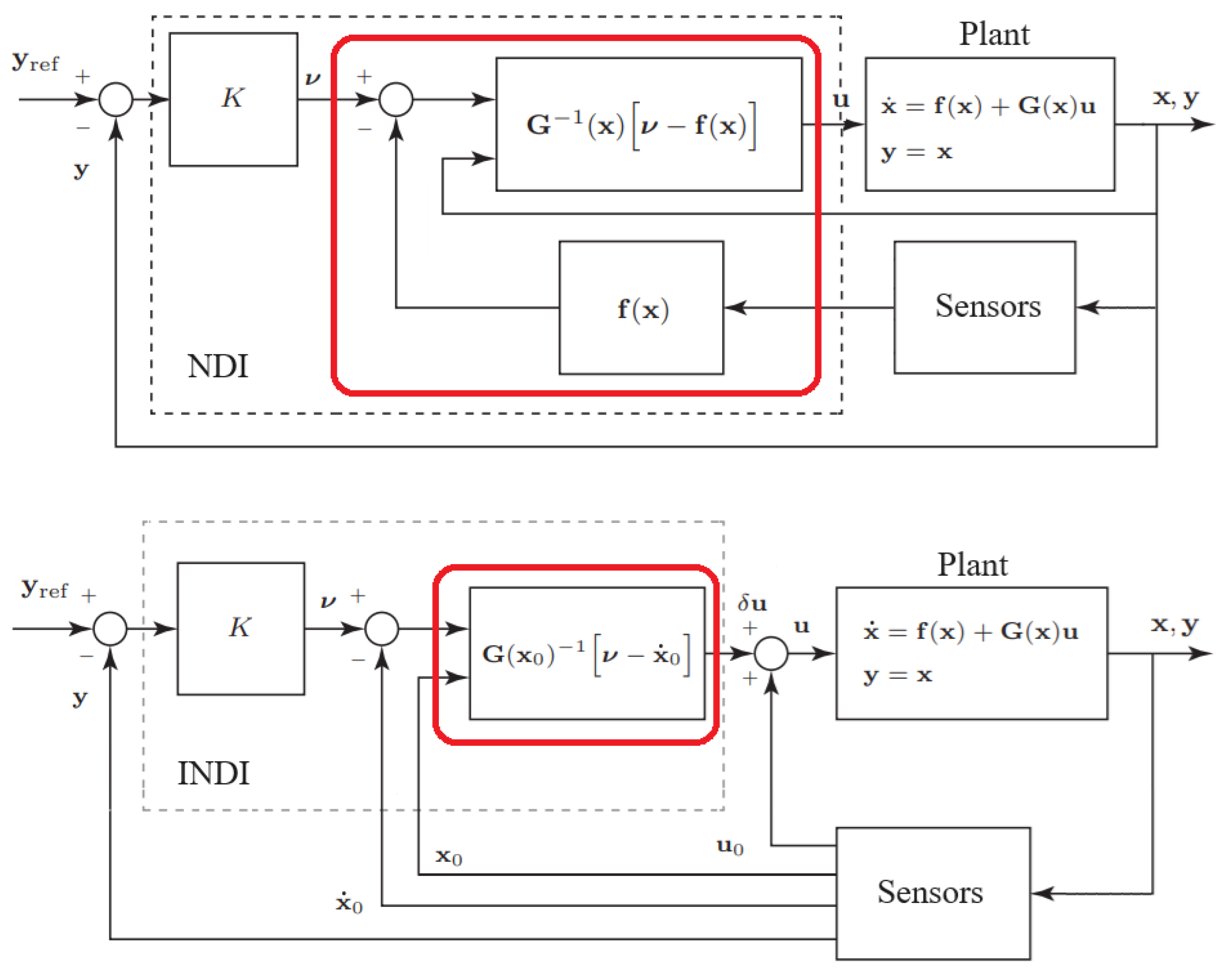
. Note that we can impose
, where
is the desired state, and
K is a constant matricial gain (
Figure 6).
In the specific scenario of a linearized airship model around a given equilibrium point, the effectiveness matrix
G corresponds to the input matrix
B of the linearized dynamics, resulting from the airship’s lateral and longitudinal decoupled models (Equations (
3) and (
4)).
Finally, note that for the classical NDI approach, the control law would be
The substitution of this equation into the dynamics of the plant (
5) leads to a perfect cancellation of the system nonlinearities, assuming that the controller has perfect knowledge of
and
.
Both the NDI and INDI principles are summarized in
Figure 6. Note that the NDI controller is much more dependent on the plant model than INDI, while INDI is more sensor-dependent than NDI.
5.2. L1 Guidance Approach for Path Following
Among the different types of missions to be executed by the airship, one important navigation problem is path following through a list of predefined waypoints to be visited at a constant altitude. Given the mission waypoints, the first task consists of defining the path passing through the waypoints. Given that airships typically fly in open-sky scenarios, obstacle avoidance may not be required, and the path can be set using straight paths linking the waypoints or, depending on the mission, using a more sophisticated optimal solution, such as the Dubins paths [
32,
33].
Once the path is defined, a lateral guidance strategy is required to ensure that the airship follows the desired path, with the LOS-based (Line-of-Sight) guidance being the standard approach [
34,
35]. However, the LOS strategy can lead to undesired errors when dealing with discontinuities in the path curvature, which is the case for straight-line paths and Dubins paths. An alternative considered in this project is the L1 guidance strategy [
19].
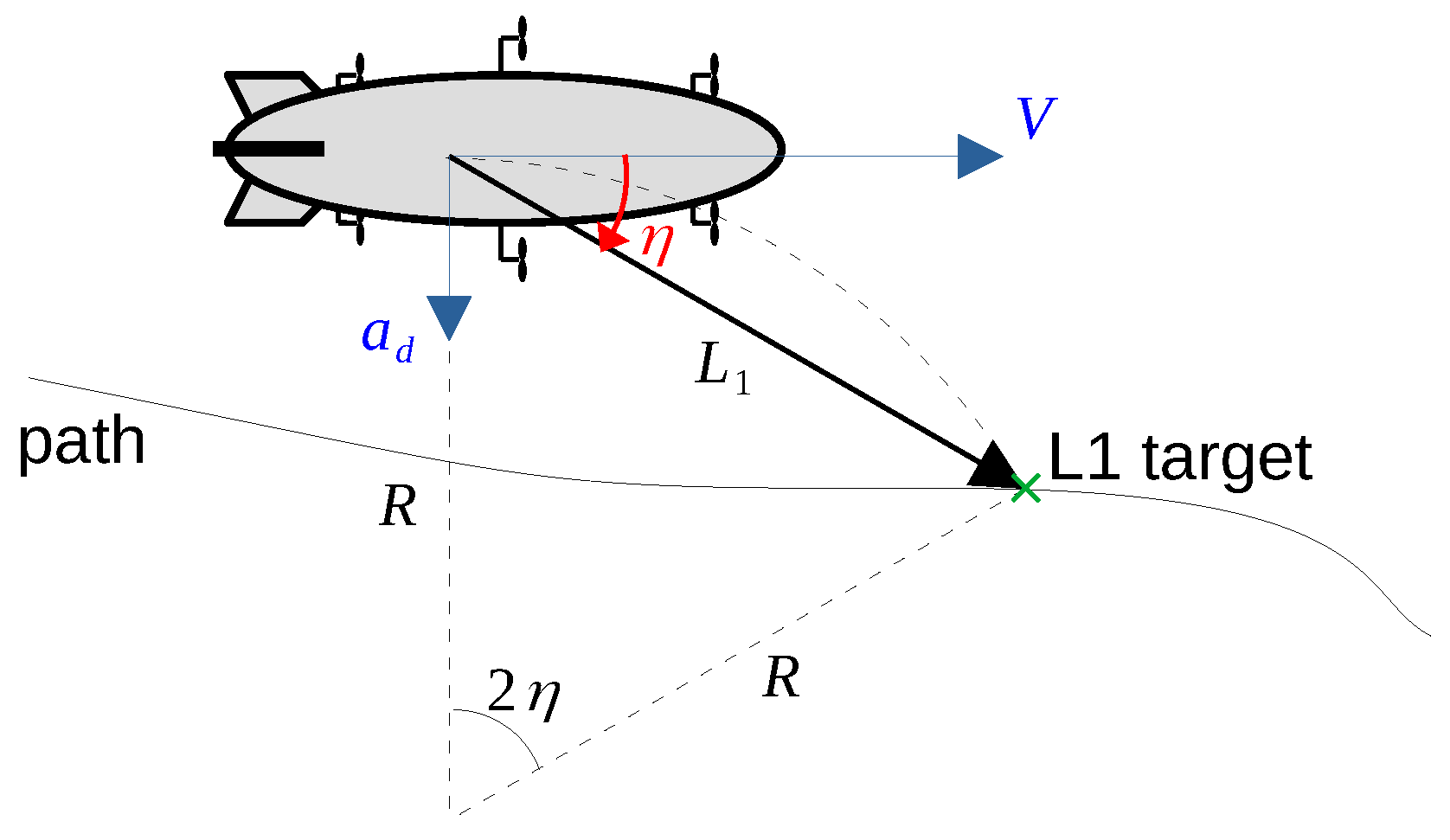
L1 guidance is a nonlinear path-following strategy that defines a circular path toward a target point located in the desired path and within an
distance from the airship, as shown in
Figure 7.
L1 guidance provides the desired centripetal acceleration
for the airship to move in the circular path to the target point. Considering
as the angle with the airship, and knowing from the geometry shown in
Figure 7 that
, the desired acceleration is given as
Some important properties of the L1 guidance strategy are the following [
19]:
The sign of the angle between the airspeed vector and the target vector defines the sign of the centripetal acceleration and, therefore, defines the direction of the turn.
The angle increases when the aircraft is far away from the path, leading to a larger acceleration. When approximating the path, the acceleration decreases, leading to a smooth approximation to the desired path.
From (
12), it is clear that the desired acceleration can be directly converted into the desired yaw rate:
The desired yaw rate provided by the L1 guidance strategy can then be used as a reference for the INDI inner loop.
6. Simulation Results
This section presents a simulation experiment for the Noamini waypoint path-tracking problem when applying the INDI controller at the low level and the L1 algorithm at the high-level guidance.
The mission is usually defined by the user for a set of consecutive waypoints i indicated by a table of reference vectors , where defines the 3-D coordinates of a given waypoint i (with as the negative of the altitude), indicates the heading angle to the next waypoint (with 0 for a straight flight segment and rad for an arc of a circle), and is the reference airspeed for the segment.
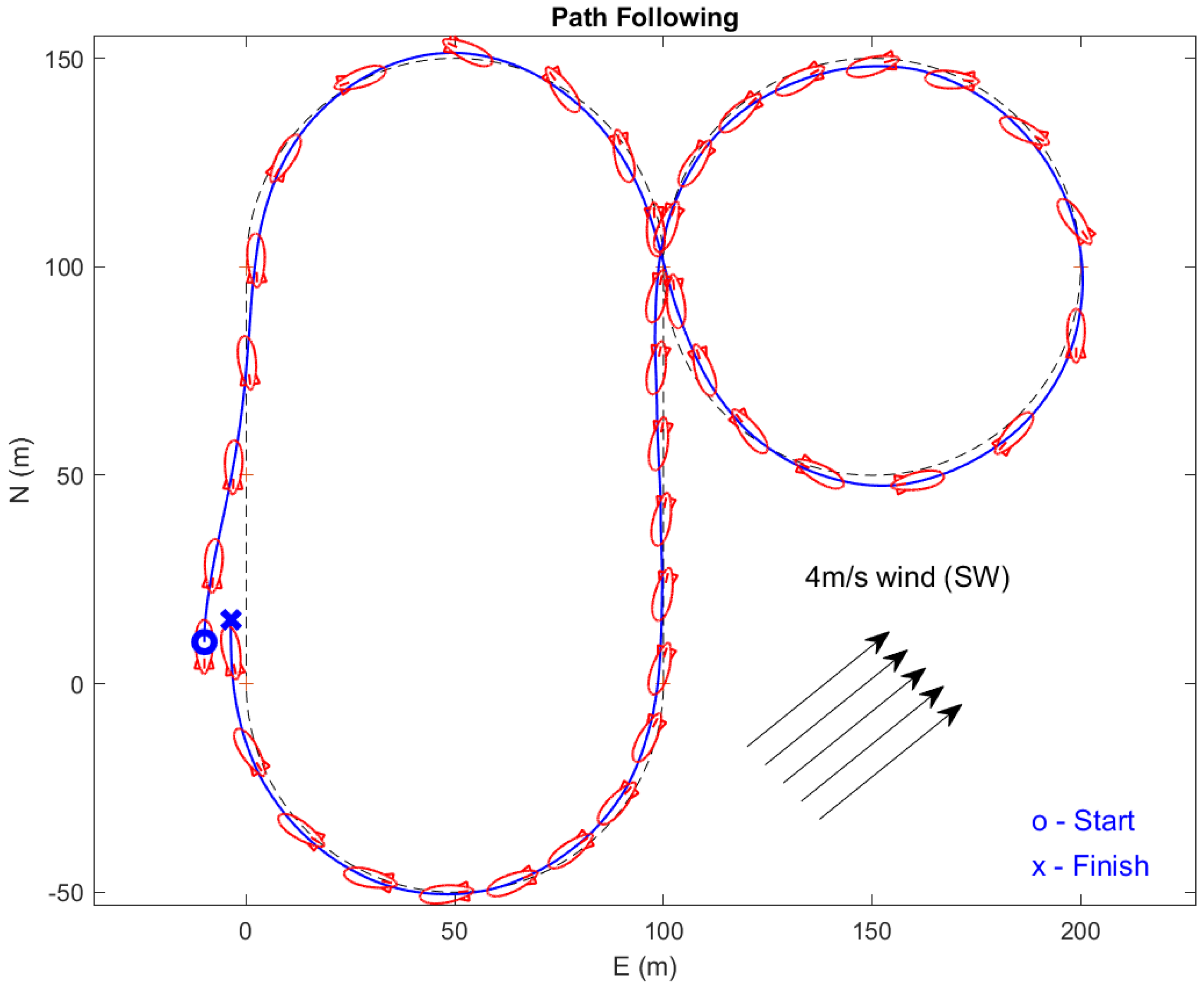
For this simulation, we assumed a +1 kg weighting mass, a reference airspeed of 10 m/s and a reference altitude of 50 m. We tested the four-motor configuration with a control rate of 100 Hz. We also considered a constant wind of 4 m/s blowing from the southwest at 45 deg with the south, as shown in
Figure 8, added to a continuous Dryden turbulence (
= 4 m/s).
The airship starts at
(m), in a position slightly “out of the path” to be followed, which is the classic “8” configuration (
Figure 8). Note also that the reference altitude of 50 m is subject to up/down changes (
) at four different points of the path, as shown in
Figure 9.
Figure 9 shows the corresponding input/output signals for this path tracking. The four red signals show the control inputs of the elevator (
), rudder (
), aileron (
) and thrust command signal (
), corresponding to the two front and two rear propellers. Elevator peaks occur to increase/decrease the pitch angle (
) at the points where an altitude change (
) is requested, around the 50 m reference. The airspeed (
) is kept around 10 m/s, while the ground speed (
u) varies between 7.5 and 12.5 m/s, as the airship faces the wind in different directions. This ground velocity variation can easily be noted by the changes in the airship stamps along the path, printed at constant time intervals. A face wind causes a decrease in the speed, while a tailwind forces it to increase.
The thrust command (
) stands around 0.4 to 0.5, with two main peaks that occur at the instants where a larger lateral velocity
v appears (as well as the sideslip angle
). The tail deflections of the rudder and aileron, although noisy due to the gust presence, act to ensure the necessary turning rate for the circular paths. The lateral acceleration command, which comes from the L1 guidance algorithm, generates the necessary yaw-rate reference (
r) to obtain a smooth path, with smooth changes in the yaw angle (
), and the minimum lateral error in path tracking, despite the strong wind and turbulence. In the same subplot of the yaw angle (
), we show, in orange color, the yaw angle for the “no wind” case. It is interesting to note the compensation angle in the “wind case”, with the classic “crab moving” of the airship under a crosswind to minimize the sideslip angle. This is particularly evident in
Figure 8 in the straight parts of the path.
7. Conclusions
This paper proposes a new kind of airship actuator configuration for surveillance and environmental monitoring missions. We present the design and application of a six-propeller electrical airship with independent tilting propellers (up to 360 degrees) that can be used in two-, four- or six-motor configurations, as well as with differential propulsion in front/rear, left/right or cross configurations.
The use of differential propulsion in three pairs of motors distributed around the envelope improves the airship lateral control, as well as the torque generation used to compensate for wind disturbances, and further provides faster yaw/pitch maneuvers, both for hover (or low speeds) and for cruise flight.
The proposal of this new airship concept with increased maneuverability is tailored for a specific class of semi-autonomous airships designed for environmental monitoring, a context where both the area coverage and detailed local data acquisition are important.
Finally, we developed a high-fidelity airship simulator for the Noamini airship, which was used to test and validate a control/guidance approach. We designed an Incremental Nonlinear Dynamic Inversion (INDI) approach for the velocity/attitude control of the airship, which is commanded by a high-level L1 guidance algorithm, which was used for a simulated waypoint-tracking mission under wind and gust disturbances.


