Abstract
In satellite health management, anomalies are mostly resolved after an event and are rarely predicted in advance. Thus, trend prediction is critical for avoiding satellite faults, which may affect the accuracy and quality of satellite data and even greatly impact safety. However, it is difficult to predict satellite operation using a simple model because satellite systems are complex and telemetry data are copious, coupled, and intermittent. Therefore, this study proposes a model that combines an attention mechanism and bidirectional long short-term memory (attention-BiLSTM) with telemetry correlation to predict satellite behaviour. First, a high-dimensional K-nearest neighbour mutual information method is used to select the related telemetry variables from multiple variables of satellite telemetry data. Next, we propose a new BiLSTM model with an attention mechanism for telemetry prediction. The dataset used in this study was generated and transmitted from the FY3E meteorological satellite power system. The proposed method was compared with other methods using the same dataset used in the experiment to verify its superiority. The results confirmed that the proposed method outperformed the other methods owing to its prediction precision and superior accuracy, indicating its potential for application in intelligent satellite health management systems.
1. Introduction
Satellites are complex systems that contain all types of subsystems and loads with a coupling relationship. Abnormalities can easily occur and may cause systematic faults that affect services and the accuracy of satellite data and significantly impact the safety of satellites. However, satellite health management relies mainly on manual operation, which is time-consuming and laborious, with faults mostly resolved after an event. If satellite operation trends are predicted, then health assessment or anomaly detection can be performed through the design of a certain algorithm. This can allow for real-time monitoring of the satellite’s health status and the timely detection of abnormalities.
Telemetry parameter data that reflect the satellite’s operational status are measured by the satellite’s sensor configuration from satellite deployment to in-orbit operation and eventually retirement. This generates large amounts of data with different telemetry features, which can be mined and analysed to predict a satellite’s operational status. However, it is difficult to determine the features related to satellite trends for all types of telemetry feature data. Currently, feature extraction methods such as principal component analysis (PCA) [1,2,3], grey relational analysis (GRA) [4], and mutual information (MI) [5,6,7,8] are widely used to extract critical variables or information. PCA combines new variables linearly with the original variables in high-dimensional data and can centrally reflect the information in the original variables; however, this method is not suitable for non-linear data [2]. When calculating the grey degree of correlation for the GRA method, many factors affect the results, such as the adjustment order of the characteristic parameters [4]. The MI is a criterion for measuring the degree of interdependence between two random variables. However, in feature extraction, it presents two main difficulties: Identifying a suitable feature evaluation strategy and accurately estimating the MI [5]. A data-driven feature selection framework constructed by the k-nearest neighbour (KNN) method [9] is suitable for data with non-linear and irregular distribution characteristics; however, this approach can produce a “dimensional disaster”.
Current trend prediction methods mainly include statistical, mathematical, intelligence-based, and information-fusion predictions. Among them, the autoregressive moving average (ARMA), support vector regression (SVR), backpropagation (BP) neural network, and long short-term memory (LSTM) prediction models have been widely studied and applied. The ARMA prediction model is a linear model with finite parameters. For short-term predictions, the model has a high fitting accuracy [10,11]. However, this approach is unsuitable for non-linear and non-stationary sequences. The SVR prediction model, which is based on structural risk minimisation, has better generalizability for small sample training sets and higher prediction accuracy than the ARMA model [12]. However, these algorithms can be used only as short-term prediction algorithms. SVR is now widely used to solve practical problems in various fields by combining it with other algorithms [13,14,15]. BP neural networks are among the most widely used neural network models owing to their strong non-linear mapping and self-learning abilities [16,17,18]. However, slow convergence, a lack of a scientific basis for determining the hidden layer nodes, and easy convergence to local minima limit their application [19]. Deep learning is a branch of neural networks. Recurrent neural networks (RNNs) with depth and time series have been widely used as prediction models for sequence data [20,21,22]. Although RNNs can handle time series problems, they have serious gradient dispersion problems. To ameliorate the adverse effects of gradient disappearance and long-distance dependence on neural networks, the long-term memory ability of RNNs can be improved by replacing RNN chain units with long-term memory units (LSTM chains) [23]. LSTM, which uses an additional memory cell to store states, has a better ability for time series prediction than RNNs. Recently, LSTM has achieved significant success in many fields [24,25,26]. Although the LSTM model has a good predictive ability for non-linear time series [27], it takes historical time series data as input, neglects the availability of future time series data, and obviates deep data mining.
The literature confirms that trend prediction has been widely applied in many fields, and deep learning has developed into a mainstream method. Satellite operation prediction, an important aspect of satellite health management, must urgently be studied in combination with deep learning methods, which present challenges at the practical application level. Zeng et al. [28] proposed an anomaly detection framework using a causal network and feature-attention-based long short-term memory (CN-FA-LSTM) network, which is used to study causality in multivariate and large-scale telemetry data and is more sensitive to anomalies for prediction. Napoli et al. [29] developed a wavelet RNN for the multistep-ahead prediction of multidimensional time series, which was applied to the prediction of satellite telemetry data. Chen et al. [30] presented an anomaly detection model based on Bayesian deep learning without domain knowledge that is highly robust to imbalanced satellite telemetry data. Yang et al. [31] proposed an improved deep-learning-based anomaly detection method for detecting anomalous spacecraft telemetry data, which combines LSTM with a multiscale detection strategy to enhance detection performance. Although these methods effectively analyse telemetry data using deep learning, it is unclear how the telemetry data that describe certain operating conditions are obtained. Because the satellite system is complex and telemetry data are copious, coupled, and intermittent, it is difficult to predict satellite operation using a simple model.
By analysing these feature extraction methods, this study presents a method that combines KNN with MI that selects the related telemetry variables from multiple satellite variables; this method is termed high-dimensional KNN-MI (HKNN-MI). Bidirectional LSTM (BiLSTM) is a variant of LSTM that can process sequence data both forward and backwards and provide past and future sequence information for each time in the sequence [32]. Moreover, a combination of the BiLSTM prediction model and attention mechanism can determine the importance of information at each input time, and the training efficiency of the model can be improved. Therefore, in this study, a model combining an attention mechanism and BiLSTM (attention-BiLSTM) with correlation telemetry is proposed to predict the operation trend of satellites.
The remainder of this paper is organised as follows. Related works on MI, attention mechanisms, and BiLSTM deep models are reviewed in Section 2. The problem statement and proposed method are introduced in detail in Section 3. The dataset was collected from FY3E to validate the feasibility of the proposed method. Section 4 provides the results of the evaluation, which were compared to demonstrate the validity of the method. Finally, Section 5 provides conclusions regarding the approach and suggestions for further research.
2. Related Work
This section reviews the related literature on MI, attention mechanisms, and BiLSTM. The MI is used to analyse the correlation between variables, an attention mechanism is applied to assign weights based on the importance of information, and BiLSTM is used to handle large amounts of time series data.
2.1. Mutual Information
In information theory, the concept of MI represents the relationship that connects information. The MI [33] can accurately describe linear and non-linear correlations between variables. Nguyen et al. [34] proposed an approach for constructing higher-dimensional MI-based feature selection methods that consider higher-order feature interactions, which differs from most previous methods that use low-dimensional MI quantities that are effective only at detecting low-order dependencies between variables. By combining MI and a kernel function, Bi et al. [35] proposed an approach for feature selection with non-linear models by defining kernels for feature and class-label vectors. For feature selection, Zhou et al. [36] proposed MI with correlation, which combines the correlation coefficient and MI to measure the relationships between different features. Liu et al. [37] proposed using MI to obtain the correlation ranking of the tested sequence and the degradation process to obtain a strongly correlated feature subset that efficiently deletes redundant and irrelevant features.
2.2. Attention Mechanism
The attention mechanism is widely used for deep learning in many fields, such as natural language processing, finance, and mechanical engineering, and it mimics systems including the human visual attention mechanism and human cognitive system. The core idea of the attention mechanism [38] is to assign a weight; that is, to assign a high weight to important information to reasonably change the attention of the outside world toward that information, ignore irrelevant information, and enlarge the required information. Variants of the attention mechanism have been designed to solve different problems. Chu et al. [39] proposed a convolution-based dual-stage attention architecture combined with LSTM networks for univariate time series forecasting. Deep attention user-based collaborative filtering [40] mines the complex relationships between users and items for recommendation from historical data. Sangeetha and Prabha [41] proposed a multi-head attention fusion model of the world and context embedding for LSTM to analyse sentiment in student feedback. Multi-head attention is a set of multiple heads that jointly learn different representations at each position in a sequence. For speech enhancement, a DNN-based model with self-attention on the feature dimension was proposed, which can make full use of the key information in frame-level features [42].
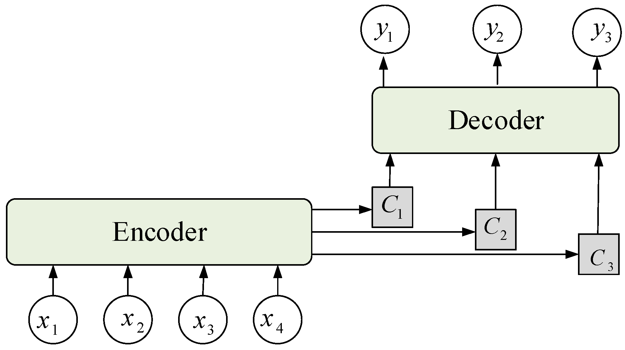
When the traditional encoder–decoder model processes an input sequence, the encoder encodes input sequence Xt into hidden vector h with a fixed length and assigns the same weight to components of the hidden vector. The decoder decodes the output based on hidden vector h. When the length of the input sequence increases, the weights of the components remain the same, and the model does not discriminate input sequence Xt, thus degrading the model’s performance. In this study, an attention mechanism was used to improve the effectiveness of the encoder–decoder model; this mechanism assigns corresponding weights to hidden vector h of the input sequence at different times, merges the hidden vector into a new hidden vector according to its importance, and then inputs it to the decoder. The encoder–decoder model with the attention mechanism is shown in Figure 1, where x1, …, x4 are the input sequences; C1, C2, and C3 are the new hidden vectors that are merged by the weight and hidden vector of the input vector; and y1, …, y4 are the output sequences.

Figure 1.
Encoder–decoder model combined with the attention mechanism.
2.3. Deep BiLSTM Model
The BiLSTM concept is derived from a bidirectional RNN that uses two separate hidden layers to process sequence data both forward and backwards. Bi-LSTM networks have successfully solved a variety of problems in many fields. A BiLSTM model based on multivariate time series data [43] was proposed for trading area forecasts to collect purchasing data and SNS data on ‘restaurants’ in the trading area for progressive learning. A short-term wind power prediction model based on BiLSTM-CNN-WGAN-GP [44] was proposed to address instability and low prediction accuracy in short-term wind power prediction. To predict heart disease, Dileep et al. [45] proposed a cluster-based bidirectional LSTM algorithm, which provided better prediction results than conventional classifiers. For implicit sentiment analysis, a BiLSTM model was proposed with multipolarity orthogonal attention [46], which outperformed the traditional method. Compared with the standard one-way LSTM, BiLSTM can obtain correlations from historical and current information, thereby improving the prediction capability [47].
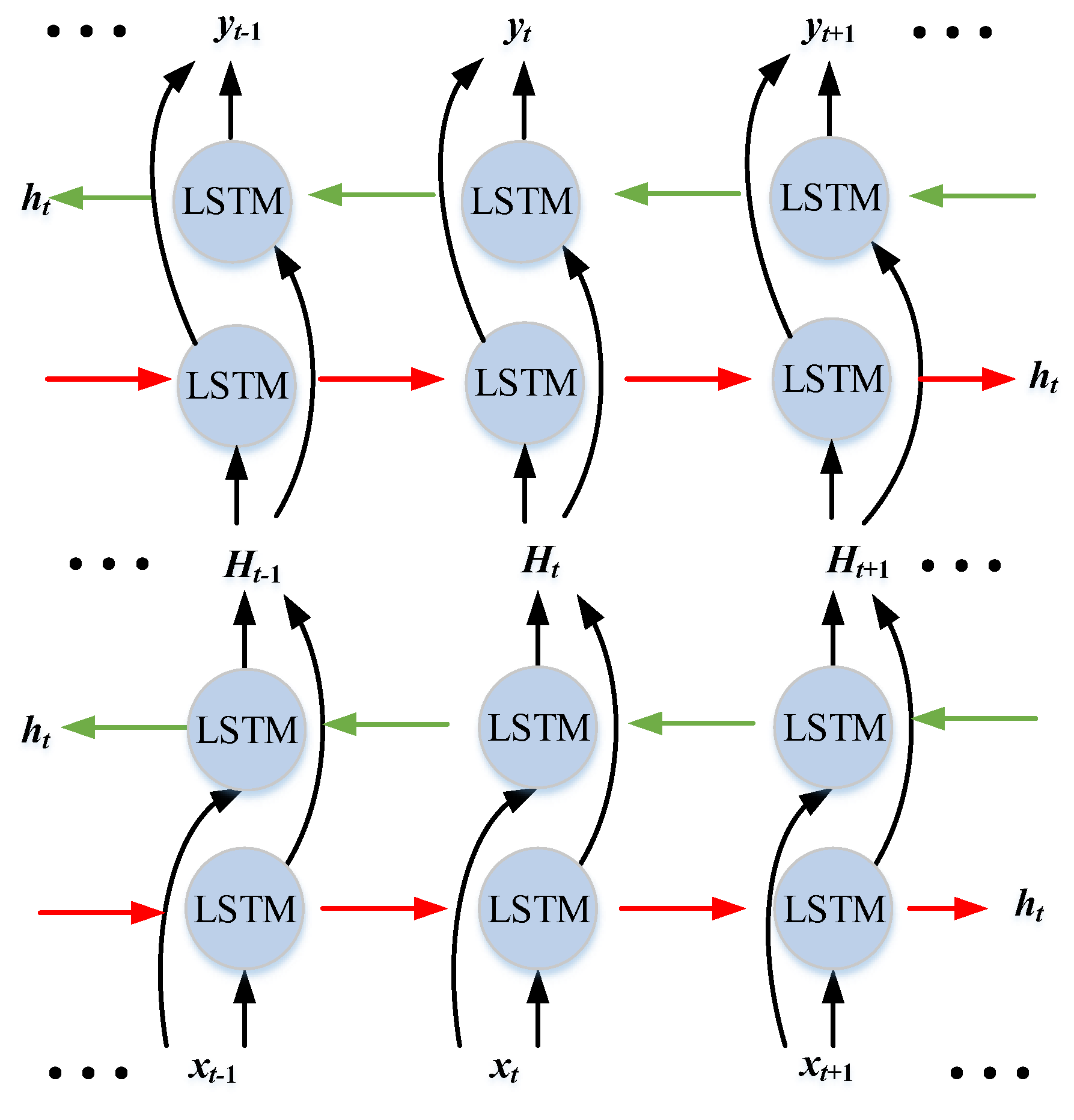
Recently, deep structures formed by stacking multiple LSTMs [48] that can be trained through multiple non-linear layers have been proven to exhibit good model training effects. The output of the previous layer is provided to the next layer as the input data for continuous learning, and additional hidden information can be learned at the learning level. Therefore, in this study, deep BiLSTM was also used for model training, as shown in Figure 2, where xt−1, xt, and xt+1 denote the input sequence; ht denotes the hidden vector; Ht−1, Ht, and Ht+1 are the outputs of the previous and input data of the next layer; and yt−1, yt, and yt+1 denote the output sequence.
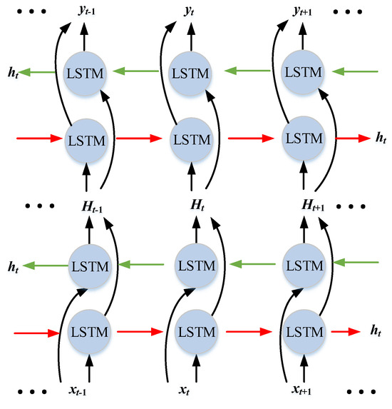
Figure 2.
Network structure of deep BiLSTM.
3. Proposed Method
In this section, the problem of predicting satellite operations is first described in detail, and a method for obtaining the optimal correlation feature for the input of the model is subsequently presented. Finally, the model architecture for predicting satellite operations is described.
3.1. Problem Statement
Satellite health management is critical for ensuring the safety of an asset. However, current health management methods are largely manual, are effective, and time-consuming. This study intends to use an artificial intelligence algorithm to solve these problems by deeply mining and analysing telemetry data, which restricts the stable operation of satellites and prevents abnormalities from being found quickly.
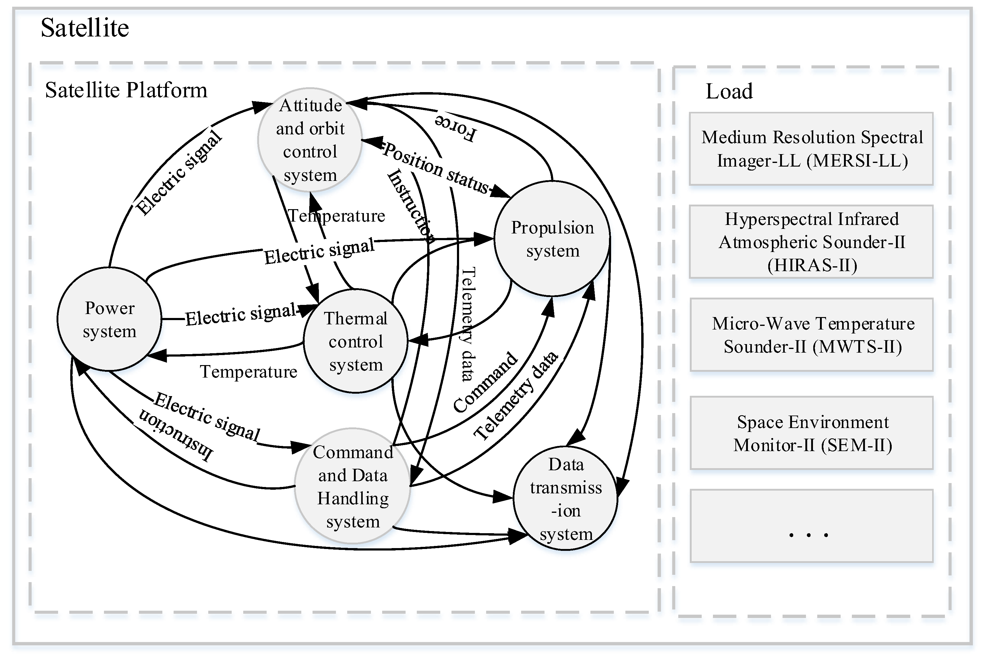
Considering the safety and reliability requirements of satellites in orbit, sensors are incorporated into the main functional modules of each key subsystem. These sensors provide telemetry parameter data for satellites from launch, throughout in-orbit operation, and until retirement. Satellite telemetry includes thermodynamic, power system, and dynamic parameters. These large amounts of telemetry data, which are stored in a time series, reflect the state of the satellite payload and the operation of the satellite subsystems. Therefore, a satellite’s operational pattern is related to the amount of temporal data. Telemetry data contain several objective laws and knowledge that can be used to predict trends. The operational trends of the satellite platform and load can be predicted based on these numerous coupled and time-related telemetry data (Figure 3 shows some parameters). However, this study faced the following challenges:
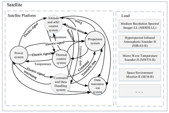
Figure 3.
Complex satellite system.
- (1)
- Feature representation is difficult because there are thousands of satellite telemetry data variables, and owing to the coupling and correlation of satellite systems, no single parameter can be used to comprehensively describe performance; moreover, determining which parameters can accurately define particular aspects of performance is challenging.
- (2)
- It is difficult to predict trends because satellite systems are complex, the telemetry signal is non-stationary and non-linear, and the telemetry parameters have three different variation patterns: stationary, abrupt, and periodic.
Traditional feature extraction methods no longer satisfy the requirements of satellite data feature representation. Therefore, selecting the features of satellite data that can accurately and comprehensively express system information is one of the key problems to be solved. After analysing the classical machine learning algorithms for time series prediction, the traditional algorithms are no longer suitable for trend prediction for complex satellites. Hence, this study proposes a new satellite prediction model.
In predicting satellite operations, we use to denote a vector of all the variables at time t, employ to represent the k-th variable series of window T, and apply to denote the target series within the length of window T. Target Y is predicted as follows:
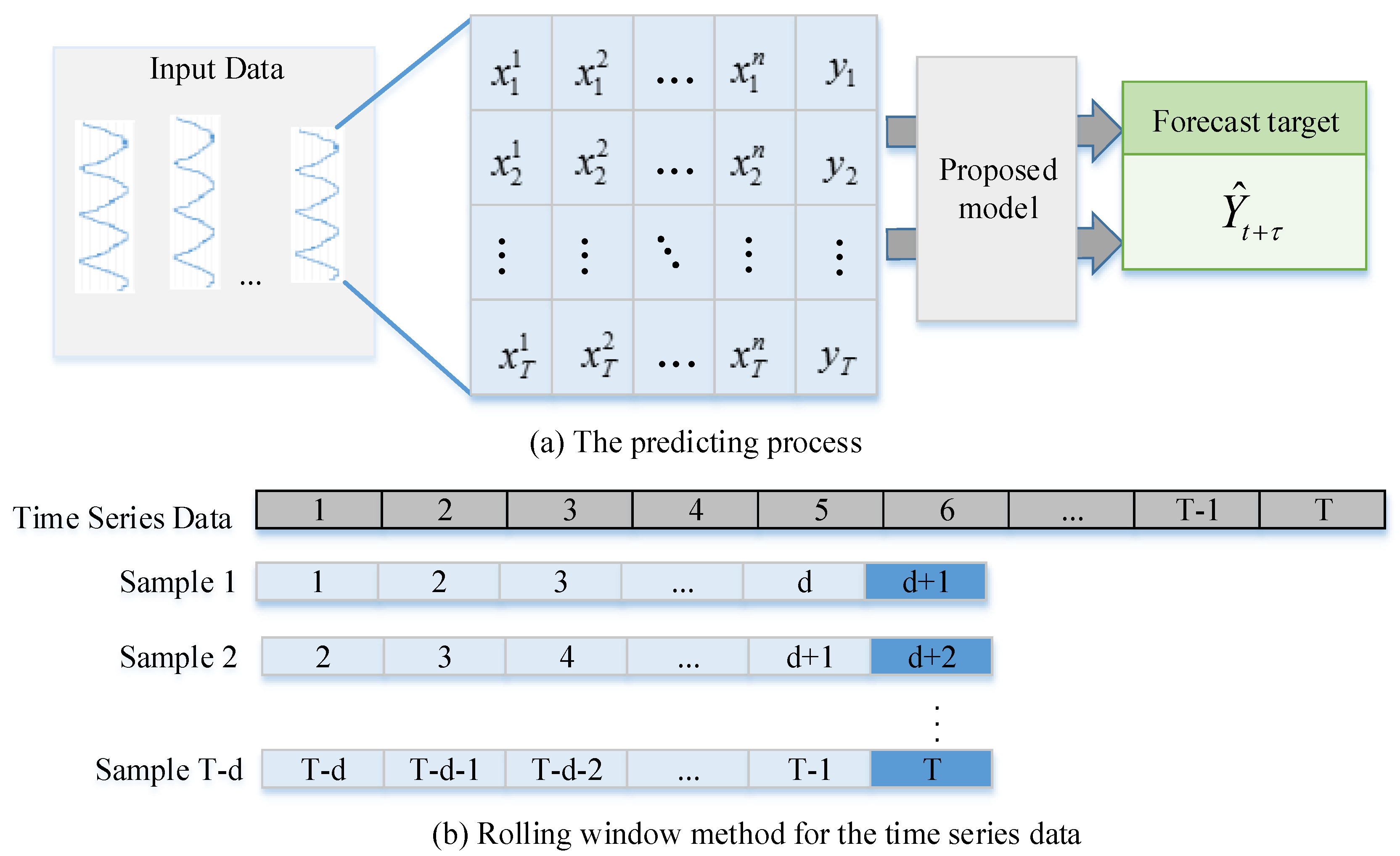
where is the predicted object in the next hours, f represents the final model trained on the historical data, Xt denotes the dataset at the moments being predicted, and is the dataset in hours before the moments being predicted. Figure 4 shows the prediction process and how the sliding window mechanism operates. In Figure 4a, the time series data are considered the input data for the proposed model. In Figure 4b, the first d points of a sequence are regarded as the input, and d + 1 is labelled as the target.
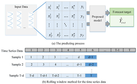
Figure 4.
Prediction process and rolling window mechanism.
3.2. Telemetry Correlation Analysis Based on the HKNN-MI Dataset
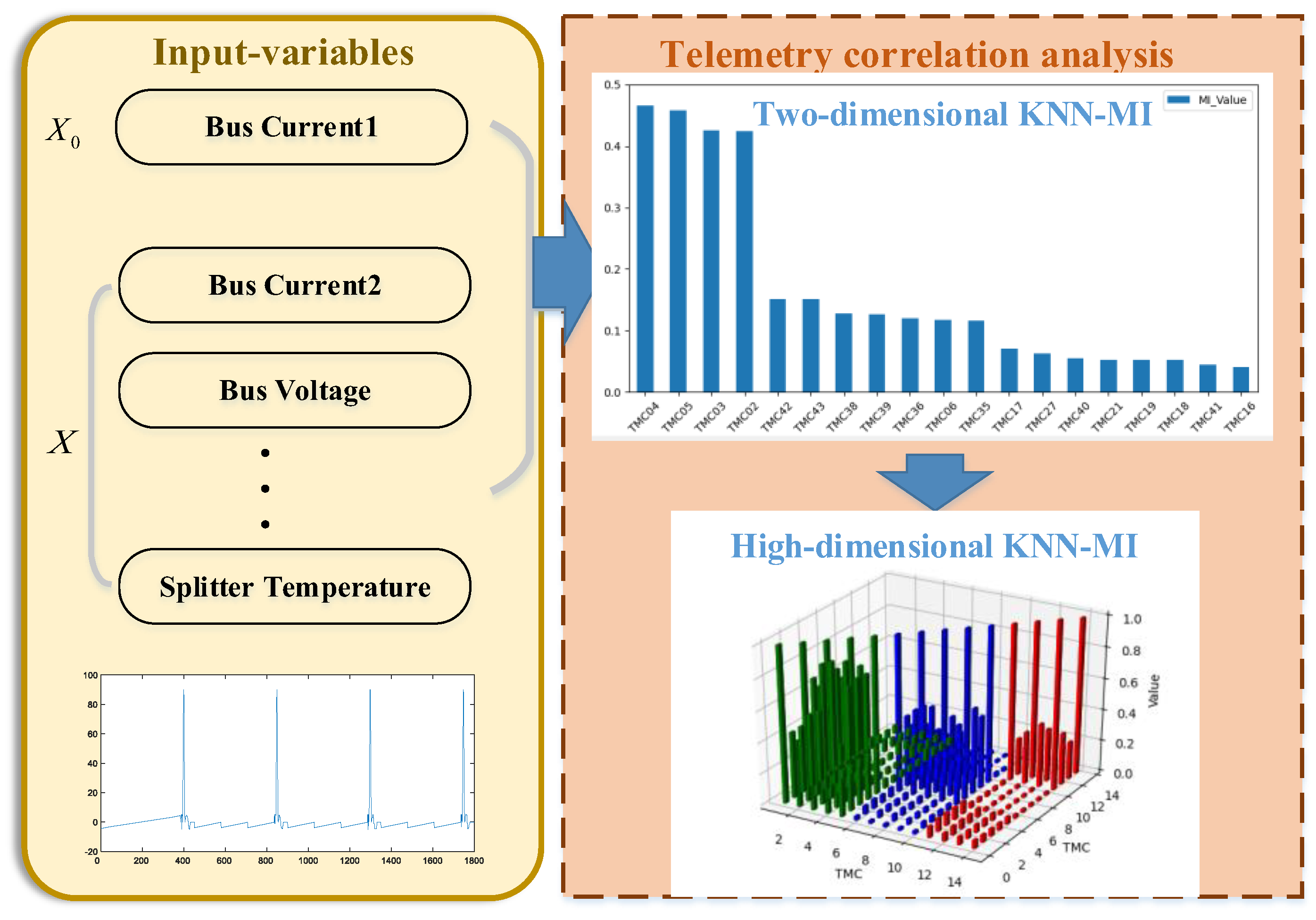
Satellites with complex structures contain a variety of loads and many types of telemetry data. Determining which variables are related to the prediction of the satellite or load operation is difficult, and the telemetry feature variables to be selected are extremely large. Therefore, we propose the KNN-MI method (Figure 5), which selects the correlation of multivariate time series variables to obtain a set of related variables, and the two-dimensional KNN-MI method is extended to estimate the MI between high-dimensional feature variables, i.e., high-dimensional KNN-MI. Moreover, a cumulative search strategy is used to obtain the optimal ranking of all features, and weakly correlated features are eliminated. Then, redundant features are eliminated using the cross-search strategy, and an optimal correlation feature subset is ultimately formed. The specific process is as follows:
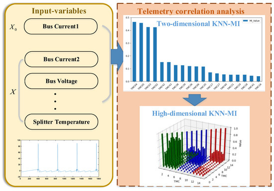
Figure 5.
Telemetry correlation analysis process.
- (1)
- Determine a strongly correlated feature X0 according to the satellite subsystem or payload to be predicted and set the k value and number of irrelevant features.
- (2)
- Calculate the high-dimensional MI of all input features X and X0 and save it in an array.
- (3)
- Sort the array according to the MI value; the feature corresponding to the maximum MI is considered the first correlation feature X1, followed by the second correlation feature X2.
- (4)
- The weak correlation features are eliminated according to the pre-set number of irrelevant features, and the strong correlation feature subset is obtained.
- (5)
- Calculate the MI between two pairs in the correlation feature set, determine the feature group corresponding to the maximum MI, and obtain the optimal strongly correlated feature subset.
3.3. Combining Attention and BiLSTM for Satellite Operation Prediction
Satellite operation is characterised by telemetry data transmitted from satellites with certain spatial and temporal correlations. BiLSTM can solve the problem of long-term dependence between current and past moments and address the correlation between current and future moments. Accordingly, this study introduces BiLSTM to predict satellites’ operational trends. Moreover, the attention mechanism is employed to assign greater weight to timeframes that have a greater impact on the prediction results.
However, in practical applications, we cannot obtain future time series data; therefore, this study presents the use of the LSTM model to predict future trends and takes the prediction results and historical data as the input of BiLSTM. To improve the model training effect, a deep BiLSTM was designed to learn more hidden information at the training level. Figure 6 shows the workflow of the proposed method. The process consisted of two parts: telemetry correlation and prediction.
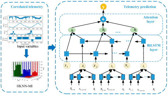
Figure 6.
Workflow of the satellite operation prediction model.
BiLSTM comprises forward- and backwards-propagating LSTM. In the LSTM structure, a memory controller is used to decide which information to forget and retain, and the input and output of information are realised through three structures: The input, forget, and output gates. Suppose that ct−1 denotes the cell state of the previous moment; ht−1 is the output of the former LSTM; and xt and ht represent the input and state outputs, respectively, for the current moment. ft, it, and ot represent the output values of the forget, input, and output gates, respectively. The updating process can be summarised as follows:
where and ct represent the candidate and current cell states, respectively. Wc, Wf, Wi, and Wo denote the weights of the candidate input, forget, input, and output gates, respectively. bc, bf, bi, and bo represent the biases of the candidate input, forget, input, and output gates, respectively. and tanh represent the sigmoid and hyperbolic tangent activation functions, respectively.
In the BiLSTM network, after telemetry correlation analysis based on HKNN-MI, the historical time series data X = [x1, x2, …, xt] are input into the forward network unit of the BiLSTM, which obtains the forward hidden layer state . The historical time series data X = [x1−n, x1−(n−1), …, x1] are used as the input of the LSTM network to predict the future time series data . The post-telemetry correlation analysis of the predicted time series data are input to the backwards network unit of BiLSTM, which obtains the backwards hidden layer states . and are expressed separately as
where is the non-linear activation function of the hidden layer, is the weight from input x of the current neuron to the hidden layer at this moment, is the weight from the state quantity at the previous moment to the current state quantity, is the output value of the hidden layer at the previous moment, and is the offset term. and are pieced together for ht, which is the hidden state of BiLSTM at timestep t. The linear combination H of BiLSTM hidden vectors with n time steps is defined as
H = (h1, h2, …, hn)
To improve the ability of the BiLSTM prediction model, a temporal attention mechanism was adopted in the decoder stage to select and weigh the relevant encoder’s hidden state across time steps. Thus, the temporal relationships of the input sequences can be learned, and the model assigns a corresponding weight to the input part during training. Supposing that the previous decoder hidden state is and the encoder hidden state is hj, the attention weights of the encoded hidden state can be computed as
Here, eij is the relationship score between and hj; the higher the value, the greater the correlation. aij is the attention coefficient corresponding to eij and is assigned to the different intermediate states hj. The vector C obtained by summarising aij and hj is input into the decoder, which calculates the prediction result through the fully connected layer the next time.
4. Results and Discussion
4.1. Datasets
FY3E is a second-generation polar-orbiting meteorological satellite and the first civil dawn-dusk orbit meteorological satellite in the world. The system includes a power system, control system, thermal control system, and attitude and orbit control system, which have 11 loads, namely, the Medium Resolution Spectral Imager-LL (MERSI-LL), Hyperspectral Infrared Atmospheric Sounder-II (HIRAS-II), and Micro-Wave Temperature Sounder-III (MWTS-III) loads. The operating trends of the power system were used to evaluate the performance of the proposed approach. The telemetry data of the power system, which were generated and transmitted from the FY3E satellite, were used to identify the method.
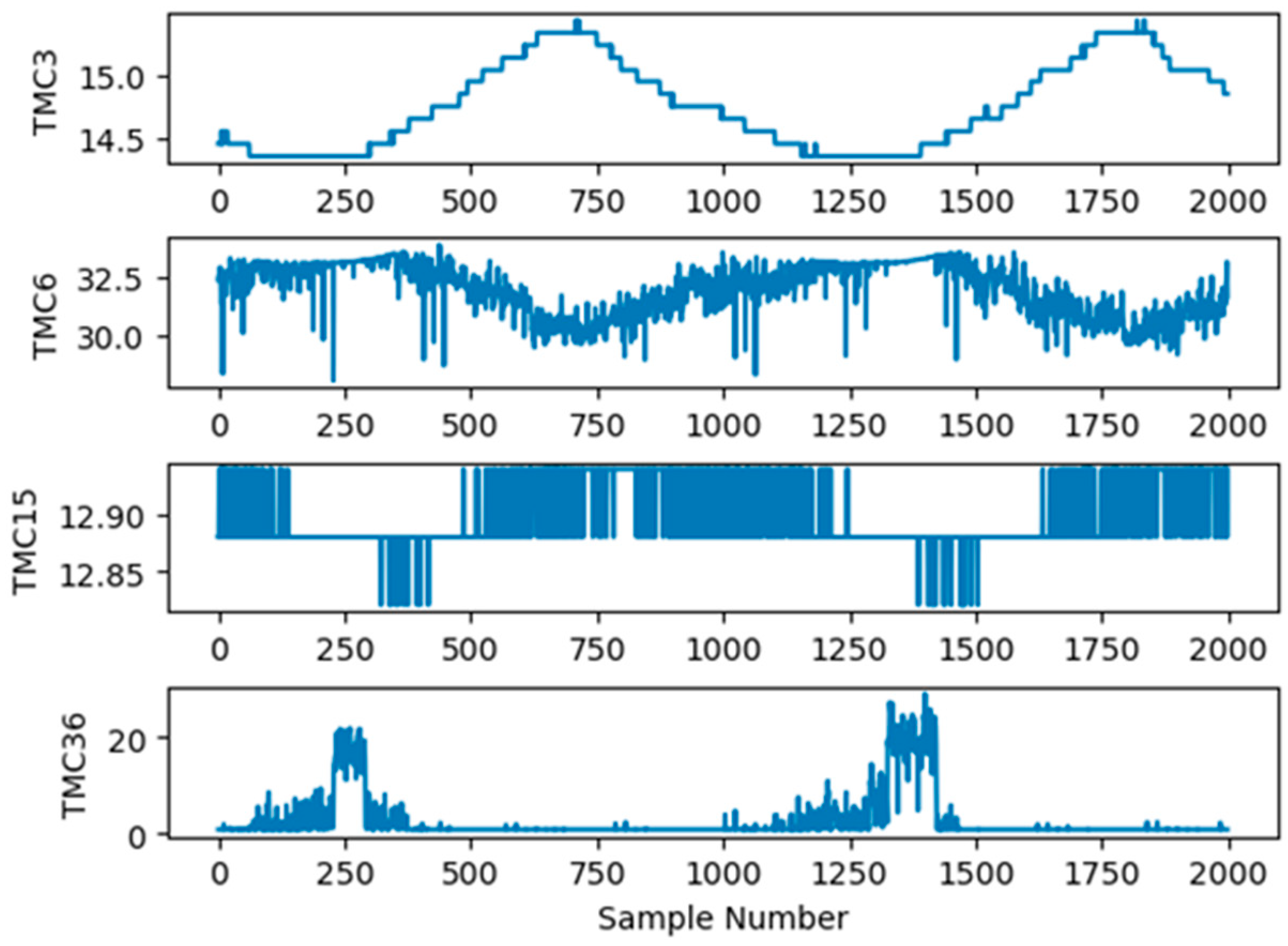
Seventy-six observation variables corresponding to the telemetry values generated from the power system of the FY3E satellite were used to predict the operational trends of the power system. Therefore, each sample dataset for trend prediction consisted of 76 variables, that is, X = [TMC1 TMC2 … TMC76], as shown in Table 1. The dataset was generated at a sampling interval of 5 s. In total, 108,708 samples were collected as training and test samples. Figure 7 shows that TMC3, TMC6, TMC15, and TMC36 changed with time from 00:00:00 to 00:03:14 on some days. As shown in Figure 7, different variables exhibited different operation trends with time.

Table 1.
Satellite telemetry variables.

Figure 7.
Changes in TMC3, TMC6, TMC15, and TMC36 with time.
4.2. Evaluation Metrics
To assess the performance of the proposed model, the mean absolute error (MAE) and root mean square error (RMSE) were calculated. The MAE is the average value of the absolute error and reflects the real situation of the prediction error. The MAE is calculated as follows:
where and yi represent the predicted and real values, respectively, at time point i and n is the number of samples. A smaller MAE indicates a more accurate prediction.
The RMSE is the square root of the square sum of the errors divided by the number of samples and is defined by Equation (15):
where n is the number of samples, yi is the actual value, and is the corresponding prediction for the target series. A smaller RMSE indicates a more accurate prediction.
The MAE and RMSE can be used to measure prediction error. The difference is that the RMSE can penalise large errors, whereas the MAE cannot. However, the MAE better reflects the actual situation of the predicted value error.
4.3. Experimental Analysis
4.3.1. Telemetry Correlation Analysis
The load, charging, and shunt currents at all levels are the most important factors in the power system of the FY3E meteorological satellite. The sum of these terms is the bus current, which is the output current of the solar array. The product of the bus current and voltage is the output power of the solar array. Therefore, the bus current is considered a focus in the power system. These parameters can also be used to determine the use of power systems in each satellite subsystem.
As mentioned, the telemetry bus current TMC1 (Bus Current1) is the strongly correlated feature X0 in the operation trend of the power system. The MI results obtained with other telemetry methods are shown in Figure 8, and only the first 45 results are displayed. In Figure 8, the horizontal axis represents each telemetry channel, and the vertical axis represents the MI values of TMC1 and the other telemetry channels. As shown in Figure 8, of the 76 main telemetries of the power system, the first 21 are appropriately selected as correlation features, and the last 55 are irrelevant.
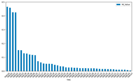
Figure 8.
Telemetry correlations.
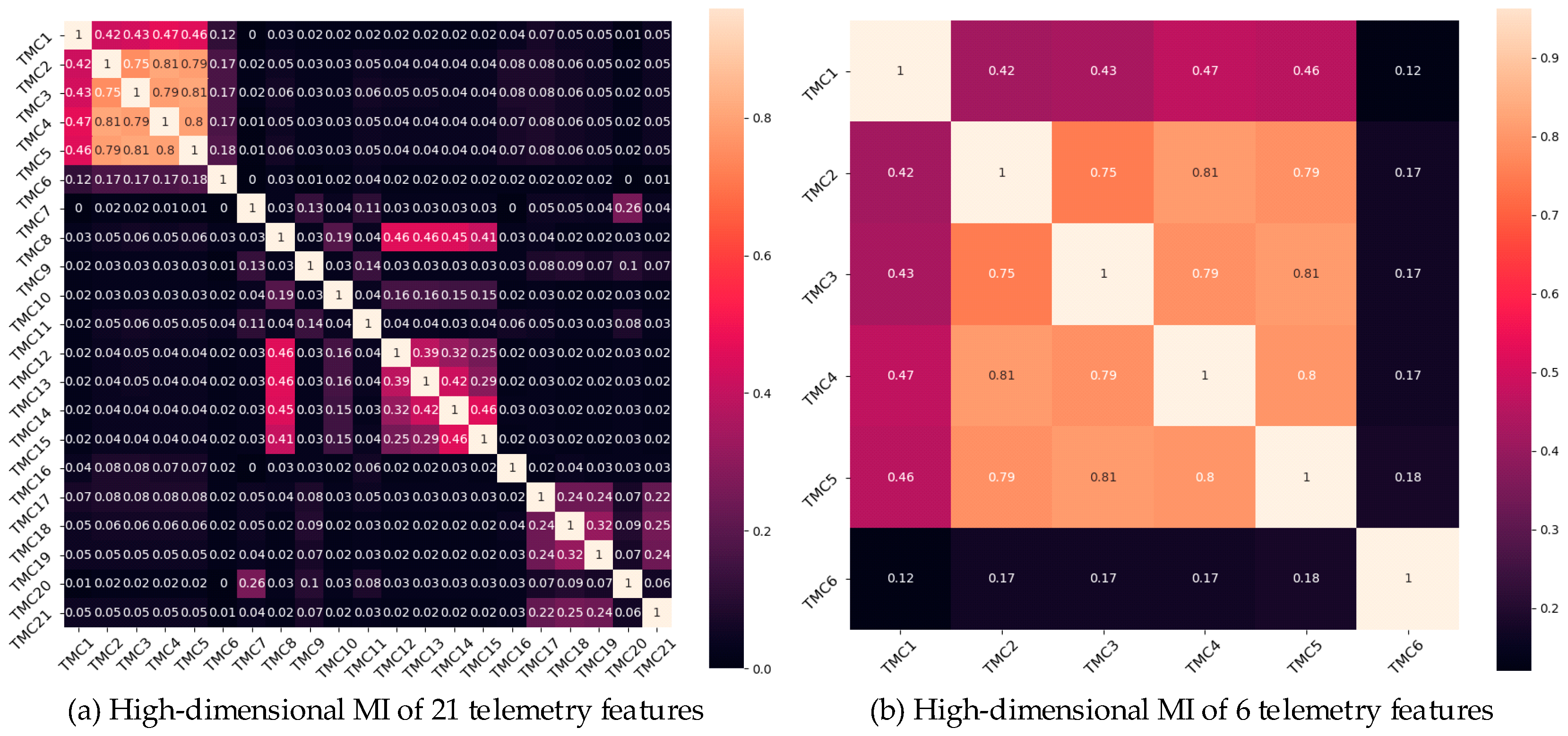
The high-dimensional MI of the 21 selected telemetry features was calculated. Figure 9 displays the MI values for 21 and the first 6 of 21 telemetry channels, as shown in Figure 9a and Figure 9b, respectively. As shown in Figure 9, TMC1, TMC2, TMC3, TMC4, and TMC5 had high correlations; TMC8, TMC12, TMC13, TMC14, and TMC15 had high correlations; and TMC17, TMC18, TMC19, and TMC21 had high correlations. These telemetry channels profoundly affect the operations of power systems. To explain this matter more intuitively, the MI connecting these 14 telemetry devices (including itself) is shown in Figure 10. The different coloured bars indicate that these telemetry variables are closely related. These results suggest that the operation of the power system can be characterised by these telemetry channels. Therefore, TMC1, TMC2, TMC3, TMC4, TMC5, TMC8, TMC12, TMC13, TMC14, TMC15, TMC17, TMC18, TMC19, and TMC21 are considered important features for predicting the future operation of a power system.
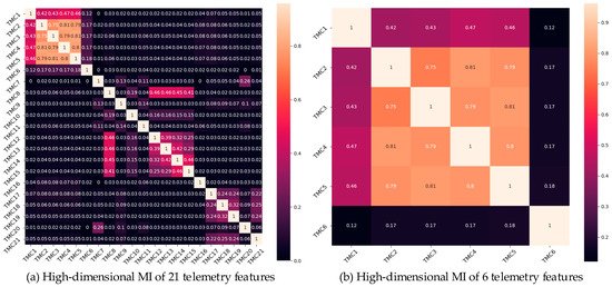
Figure 9.
MI values of the telemetry channels.
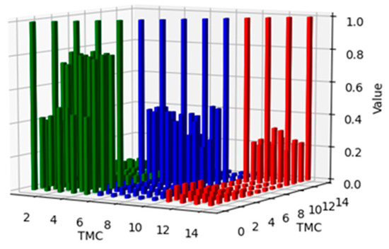
Figure 10.
Diagram of high-dimensional MI.
4.3.2. Analysis of Parameters
The dataset was normalised to reduce the impact of dimensional differences in its characteristics. After reprocessing, the dataset was partitioned using the roulette method, with 70%, 20%, and 10% as the training, verification, and test sets, respectively. Two experiments were conducted to evaluate the performance of the proposed method. In Part 1, an algorithm was employed to determine the optimal hyperparameters. Part 2 used a fixed hyperparameter value. The results showed that the proposed method achieved the best performance.
Because the experimental parameter settings had a significant impact on the results of the model training, the results of the final experiment after adjustment are shown in Table 2. The number of different hidden units had a considerable influence on the prediction performance of the designed model. Furthermore, on the sample, the training accuracy was highest when using 128 hidden units, 20 epochs, the Adam optimiser [49], a dropout rate of 0.5, a batch size of 8, and a learning rate of 0.0001.

Table 2.
Parameter settings of our model.
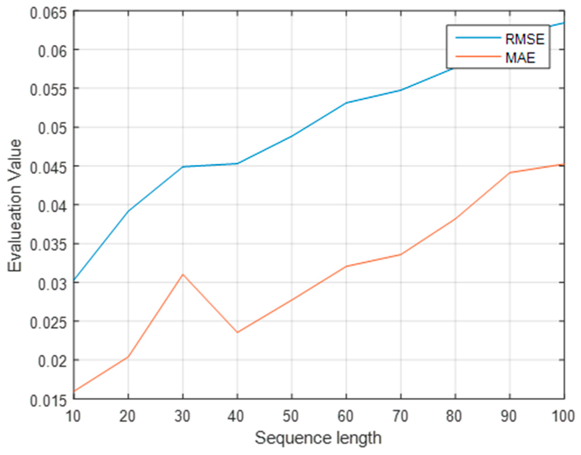
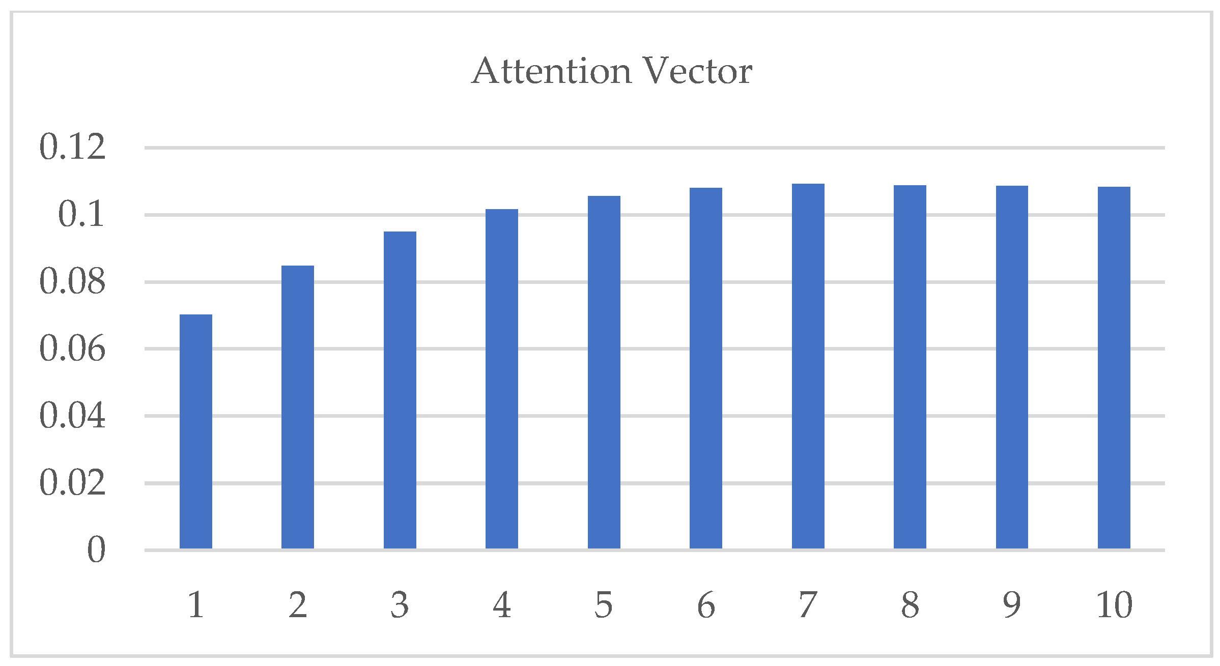
Because the input sequence contains information at multiple points before the prediction point, the length of the input sequence must be determined. Consequently, the model can simplify the calculation process and shorten the calculation time while ensuring accuracy. The experiments were conducted when the lengths of the input sequences were 10, 20, and 100. The lowest MAE and RMSE values were obtained with a length of 10. Moreover, the forecast accuracy was the highest, as shown in Figure 11. As shown in Figure 12, for the 10 input sequences, the attention vector was applied to the output of the BiLSTM layer, with the attention mechanism as a function of the input dimensions.

Figure 11.
Evaluation values for different sequence lengths.

Figure 12.
Attention vector applied to the output of the BiLSTM layer.
4.4. Performance Evaluation
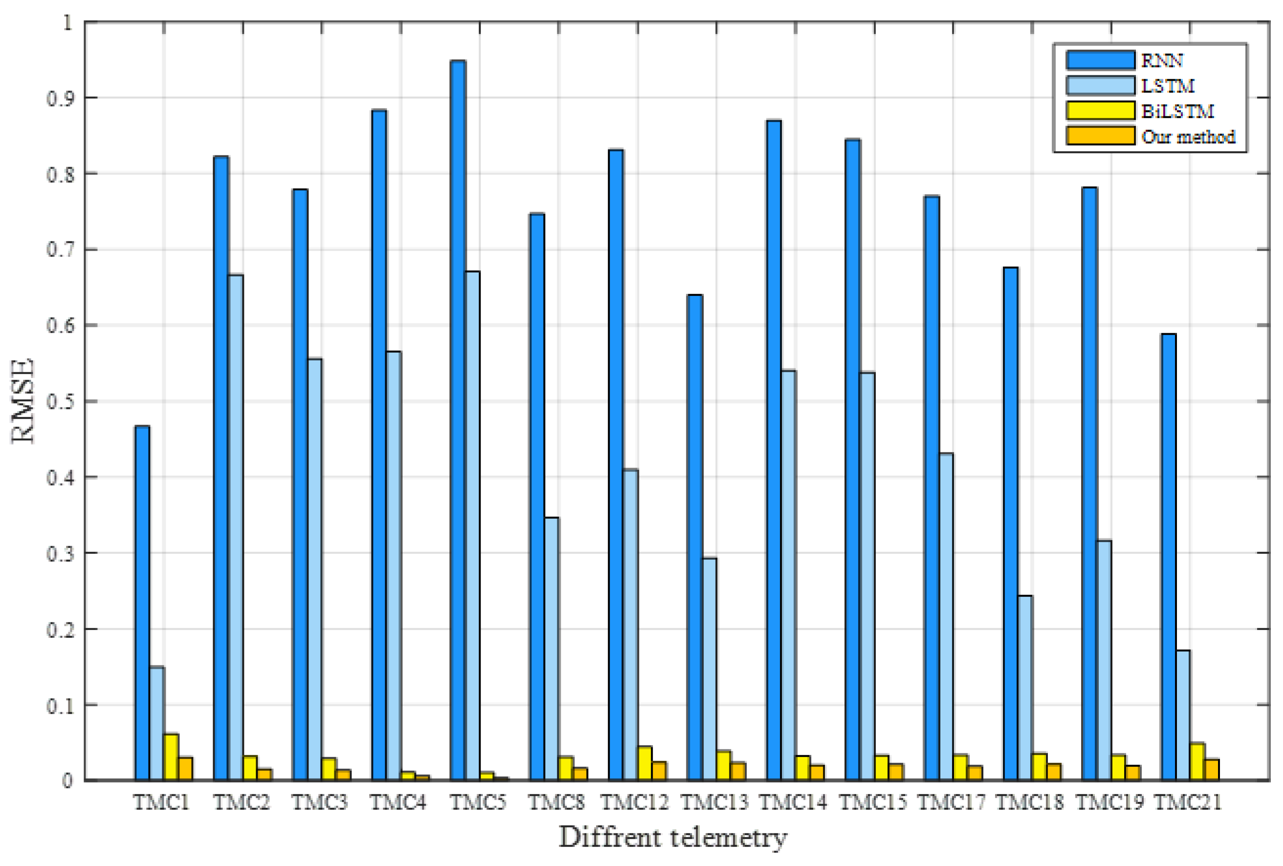
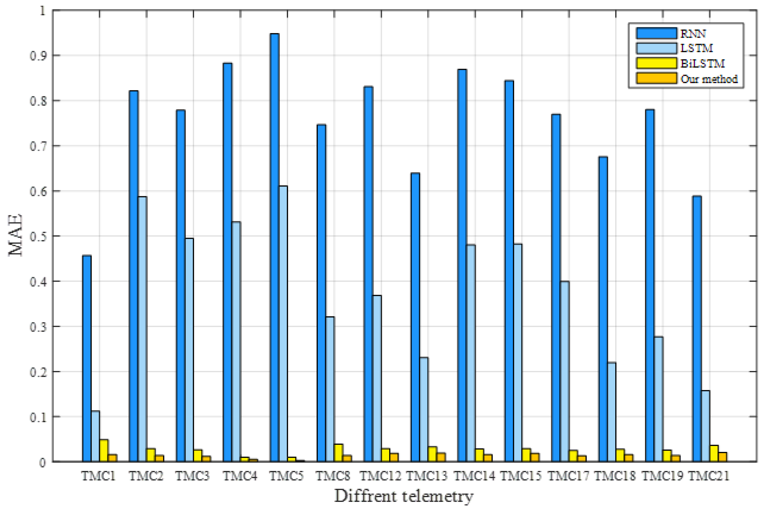
To verify the effectiveness of the proposed method, experiments were conducted to compare the three baseline models, BPNN, RNN, and LSTM, using the same training and test data in an identical operating environment. All the experiments were conducted using an Intel (R) Core (TM) i7-1.99 GHz, 8.00 GB RAM, and Windows 10 platform. The development environment included Python 3.6 and PyTorch 1.0.1.
In the experiment, TMC1, TMC2, TMC3, TMC4, TMC5, TMC8, TMC12, TMC13, TMC14, TMC15, TMC17, TMC18, TMC19, and TMC21 characterised the operating conditions of the satellite power system. The training dataset was used to train the model, the verification dataset was used to optimise its parameters, and the trained model was applied to predict the test dataset for all models. The RMSE and MAE of each method were calculated according to the real and predicted values. The prediction results of these methods are listed in Table 3. The best assessment results for each telemetry service are shown in bold. Our model attained the lowest RMSE and MAE values, indicating its superiority. To further visualise the prediction performance, Figure 13 and Figure 14 compare the RMSE and MAE values, respectively, of the telemetry methods that represent the operation of satellite power systems. These results confirm that, in terms of predicting satellite operation trends, the proposed model outperforms the classical methods.

Table 3.
Prediction performance comparison of various models.

Figure 13.
Comparison of the RMSEs for different methods.
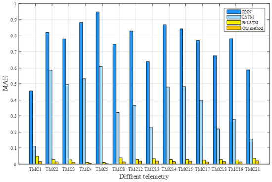
Figure 14.
Comparison of MAEs for different methods.
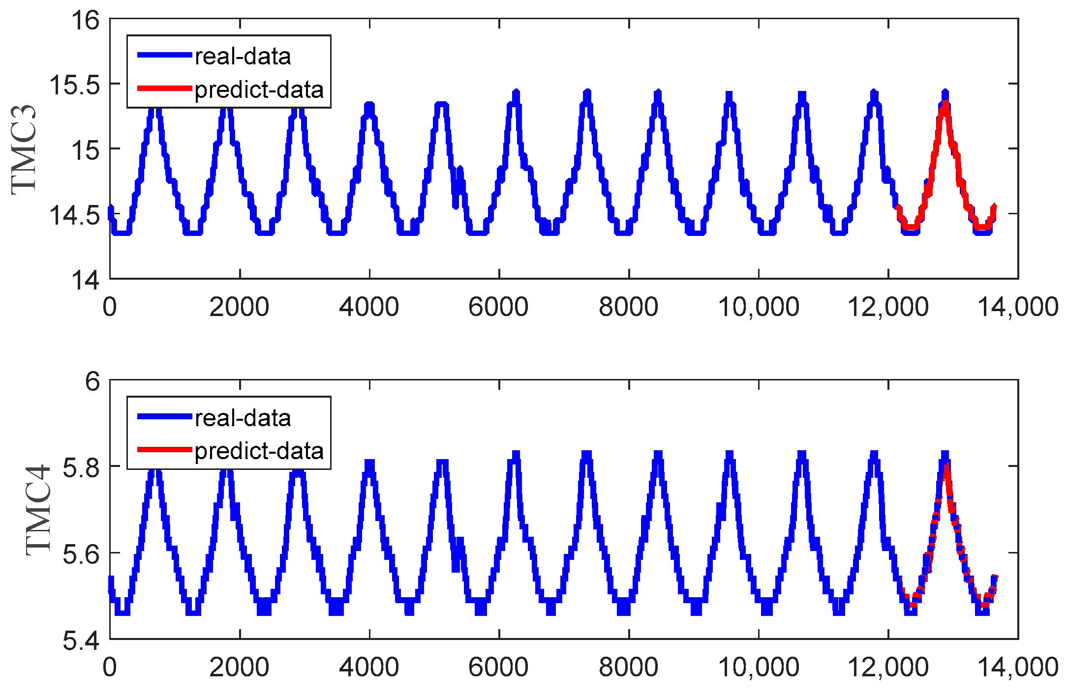
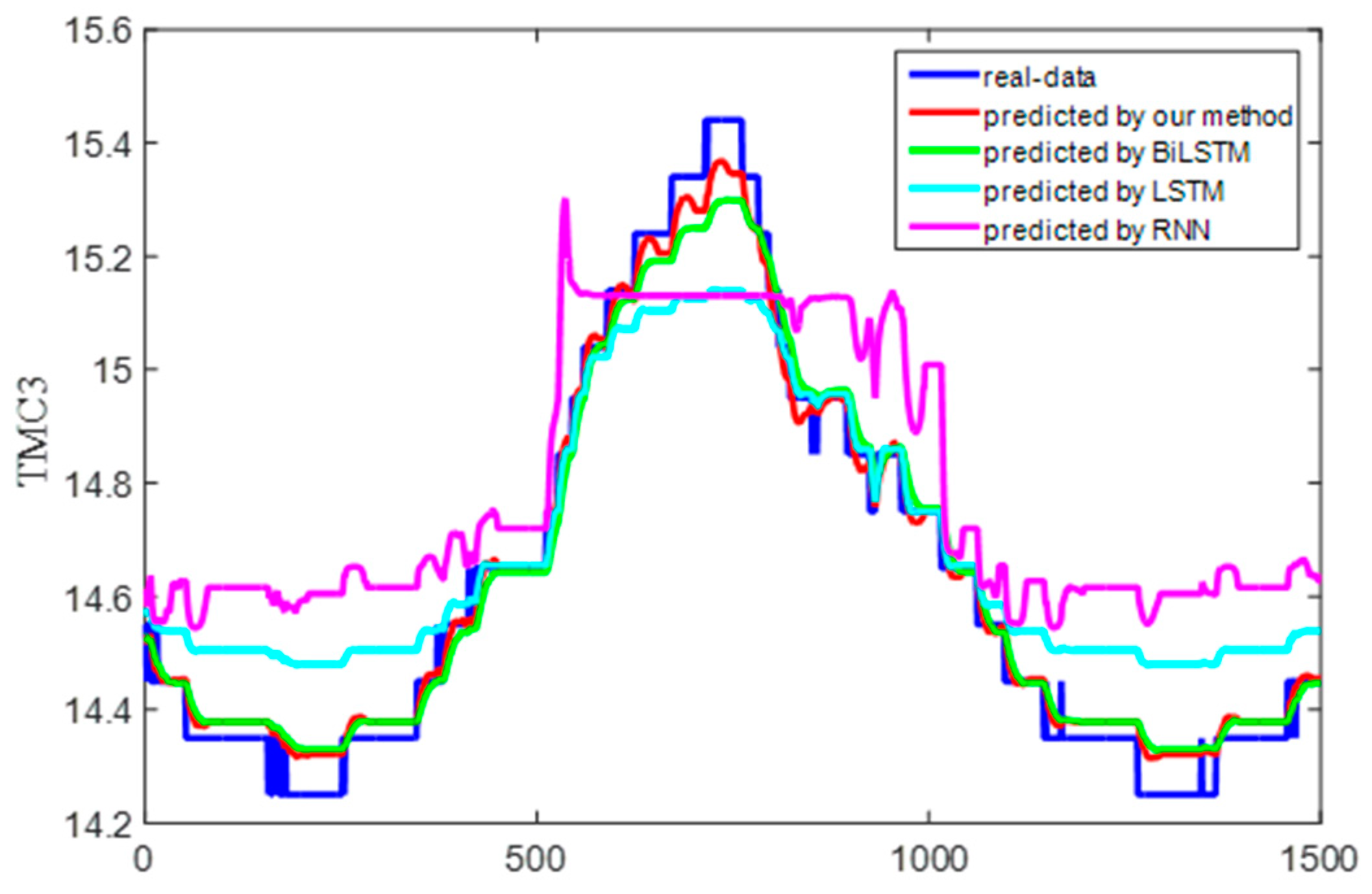
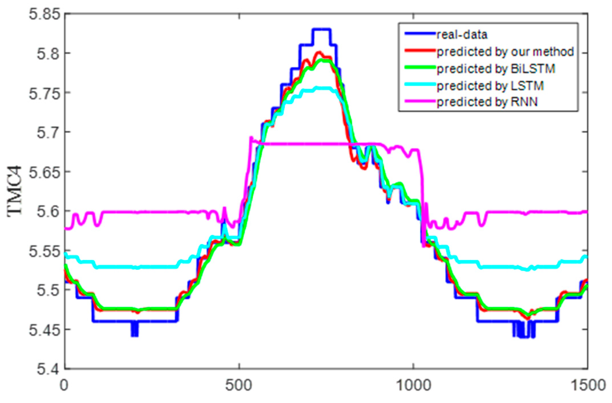
Figure 15 shows the predicted and real value curves of our model for TMC3 and TMC4. The samples obtained by the sliding window were input into the trained model for prediction, and a single predicted value was obtained each time. The predicted values were obtained by combining the predicted values for each sample. The prediction trajectory was formed using an iteratively trained model. To better represent the prediction results, the curve is enlarged, as shown in Figure 16, on the same dataset as in Figure 15. Moreover, the same dataset was used to compare the predictions of our method with those of classical algorithms, as shown in Figure 17 and Figure 18, which intuitively show each degree of deviation through the prediction curves of all algorithms and the real curves for TMC3 and TMC4. Evidently, our algorithm was superior to the other algorithms. Therefore, the proposed model is effective and feasible for accurately predicting satellite operations.
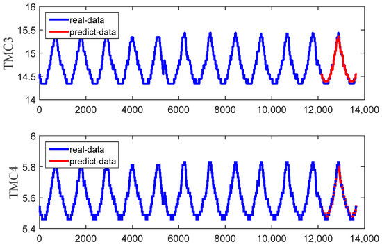
Figure 15.
Predicted and real value curves.
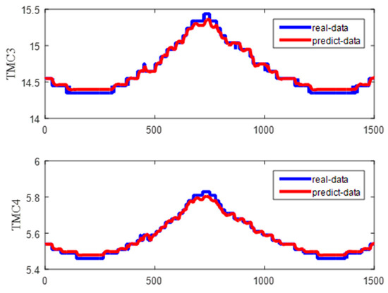
Figure 16.
Enlarged curves of the predicted and real values.

Figure 17.
Prediction and real curves for the entire algorithm for TMC3.

Figure 18.
Prediction and real curves for the entire algorithm for TMC4.
5. Conclusions
To identify abnormalities early and predict a satellite’s operational status, this study proposed an attention-BiLSTM model with correlation telemetry. The BiLSTM prediction model connected to the attention mechanism can determine the importance of the information at each input time, and the training efficiency of the model can be improved. The HKNN-MI method was applied to select relevant telemetry variables from multiple variables in the satellite telemetry data. The superiority of the proposed model over the RNN, LSTM, and BiLSTM models was verified using a dataset from the power system of the FY3E meteorological satellite. The experimental results indicated that the proposed model achieved state-of-the-art results in the prediction of satellite operations.
Further research will be conducted to improve upon the existing methods to achieve a unified model for feature selection and prediction and obtain more accurate results based on larger datasets. The application of this method to real-time operation data from satellites rather than historical datasets will also be investigated, for which the occurrence of satellite anomalies can be predicted in advance. At the same time, we also need to consider whether the algorithm is set on the satellite or the ground system. Suppose the response time for faults is extremely high. In that case, the application of satellite may be more suitable, as it can monitor the status of the satellite in real-time. However, the resources on satellite are limited, and the model needs to be optimized to adapt to the limitations of energy, computing power, and storage space. The ground system can utilise more abundant resources to handle more complex tasks. In addition, the ground system is easier to maintain and update, which helps maintain the long-term stable operation of the system. The maintenance cost of a satellite is high, and once deployed, the system must operate autonomously as much as possible. Therefore, we will consider experimental applications on ground systems.
Author Contributions
Conceptualisation, Y.P.; funding acquisition, Y.P.; methodology, Y.P.; software; writing—original draft, Y.P.; data curation, S.J.; investigation, S.J.; project administration, S.J.; supervision, L.X.; visualisation, L.X.; revising the manuscript, J.S. All authors have read and agreed to the published version of the manuscript.
Funding
This work was funded by National Natural Science Foundation of China with grant number [62306082] and National Key Research and Development Program of China with grant number [2023YFB3907502].
Data Availability Statement
The data supporting this study are the actual operational data from in-orbit satellite, which is private information and therefore not disclosed here.
Acknowledgments
The authors of this paper would like to thank the team from Operation Control Center of National Satellite Meteorological Center for their support of this research.
Conflicts of Interest
The authors declare that there are no conflicts of interest.
References
- Thomas, M.; De Brabanter, K.; De Moor, B. New bandwidth selection criterion for Kernel PCA: Approach to dimensionality reduction and classification problems. BMC Bioinform. 2014, 15, 137. [Google Scholar] [CrossRef] [PubMed]
- Chang, P.C.; Wu, J.L. A critical feature extraction by kernel PCA in stock trading model. Soft Comput. 2015, 19, 1393–1408. [Google Scholar] [CrossRef]
- Hemavathi, D.; Srimathi, H. Effective feature selection technique in an integrated environment using enhanced principal component analysis. J. Ambient. Intell. Hum. Comput. 2020, 12, 3679–3688. [Google Scholar] [CrossRef]
- Song, Q.; Shepperd, M. Predicting software project effort: A grey relational analysis based method. Expert. Syst. Appl. 2011, 38, 7302–7316. [Google Scholar] [CrossRef]
- Bennasar, M.; Hicks, Y.; Setchi, R. Feature selection using joint mutual information maximisation. Expert. Syst. Appl. 2015, 42, 8520–8532. [Google Scholar] [CrossRef]
- Hoque, N.; Singh, M.; Bhattacharyya, D.K. EFS-MI: An ensemble feature selection method for classification. Complex. Intell. Syst. 2018, 4, 105–118. [Google Scholar] [CrossRef]
- Bostani, H.; Sheikhan, M. Hybrid of binary gravitational search algorithm and mutual information for feature selection in intrusion detection systems. Soft Comput. 2017, 21, 2307–2324. [Google Scholar] [CrossRef]
- Kottath, R.; Poddar, S.; Sardana, R.; Bhondekar, A.P.; Karar, V. Mutual information based feature selection for stereo visual odometry. J. Intell. Robot. Syst. 2020, 100, 1559–1568. [Google Scholar] [CrossRef]
- Li, S.Q.; Harner, E.J.; Adjeroh, D.A. Random KNN feature selection—A fast and stable alternative to Random Forests. BMC Bioinform. 2011, 12, 450. [Google Scholar] [CrossRef]
- Al-Smadi, A. The estimation of the order of an ARMA process using third-order statistics. Int. J. Syst. Sci. 2005, 36, 975–982. [Google Scholar] [CrossRef]
- Kizilkaya, A.; Kayran, A.H. ARMA model parameter estimation based on the equivalent MA approach. Digit. Signal Process. 2006, 16, 670–681. [Google Scholar] [CrossRef]
- Yuan, F.; Kumar, U.; Galar, D. Reliability prediction using support vector regression. Int. J. Syst. Assur. Eng. Manag. 2010, 1, 263–268. [Google Scholar]
- Gilan, S.S.; Jovein, H.B.; Ramezanianpour, A.A. Hybrid support vector regression—Particle swarm optimization for prediction of compressive strength and RCPT of concretes containing metakaolin. Constr. Build. Mater. 2012, 34, 321–329. [Google Scholar] [CrossRef]
- Fung, K.F.; Huang, Y.F.; Koom, C.H. Coupling fuzzy-SVR and boosting-SVR models with wavelet decomposition for meteorological drought prediction. Environ. Earth Sci. 2019, 78, 693. [Google Scholar] [CrossRef]
- Gao, W.F.; Han, J. Prediction of destroyed floor depth based on principal component analysis (PCA)-genetic algorithm (GA)-Support Vector Regression (SVR). Geotech. Geol. Eng. 2020, 38, 3481–3491. [Google Scholar] [CrossRef]
- Hao, G. Study on prediction of urbanization level based on ga-bp neural network. In Proceedings of the 21st International Conference on Industrial Engineering and Engineering Management, Macao, China, 15–18 December 2019; pp. 521–522. [Google Scholar]
- Watson, J.D.; Crick, F.H.C. BP neural network-based product quality risk prediction. In Proceedings of the International Conference on Big Data Analytics for Cyber-Physical-Systems, Shengyang, China, 28–29 December 2019; pp. 1021–1026. [Google Scholar]
- He, F.; Zhang, L.Y. Mold breakout prediction in slab continuous casting based on combined method of GA-BP neural network and logic rules. Int. J. Adv. Manuf. Technol. 2018, 95, 4081–4089. [Google Scholar] [CrossRef]
- Yuan, C.H.; Niu, D.X.; Li, C.Z.; Sun, L.; Xu, L. Electricity consumption prediction model based on Bayesian regularized bp neural network. In Proceedings of the International Conference on Cyber Security Intelligence and Analytic, Shenyang, China, 21–22 February 2019; pp. 528–535. [Google Scholar]
- Metu, N.R.; Sasikala, T. Prediction analysis on web traffic data using time series modeling, RNN and ensembling techniques. In Proceedings of the International Conference on Intelligent Data Communication Technologies and Internet of Things; Springer: Cham, Switzerland, 2018; pp. 611–618. [Google Scholar]
- Lin, C.; Chi, M. A comparisons of BKT, RNN and LSTM for learning gain prediction. In Proceedings of the International Conference on Artificial Intelligence in Education, Wuhan, China, 28 June–1 July 2017; pp. 536–539. [Google Scholar]
- Wu, Q.H.; Ding, K.Q.; Huang, B.Q. Approach for fault prognosis using recurrent neural network. J. Intell. Manuf. 2020, 31, 1621–1633. [Google Scholar] [CrossRef]
- Manaswi, N.K. RNN and LSTM. In Deep Learning with Applications Using Python; Apress: New York, NY, USA, 2018. [Google Scholar]
- Poornima, S.; Pushpalatha, M. Drought prediction based on SPI and SPEI with varying timescales using LSTM recurrent neural network. Soft Comput. 2019, 23, 8399–8412. [Google Scholar] [CrossRef]
- Mtibaa, F.; Nguyen, K.K.; Azam, M.; Papachristou, A.; Venne, J.; Cheriet, M. LSTM-based indoor air temperature prediction framework for HVAC systems in smart buildings. Neural Comput. Appl. 2020, 32, 17569–17585. [Google Scholar] [CrossRef]
- Zhao, J.; Wu, J.J.; Guo, X.W.; Han, J.; Yang, K.; Wang, H. Prediction of radar sea clutter based on LSTM. J. Ambient. Intell. Hum. Comput. 2019, 14, 15419–15426. [Google Scholar] [CrossRef]
- Gundu, V.; Simon, S.P. PSO-LSTM for short term forecast of heterogeneous time series electricity price signals. J. Ambient. Intell. Hum. Comput. 2021, 12, 2375–2385. [Google Scholar] [CrossRef]
- Zeng, Z.; Jin, G.; Xu, C.; Chen, S.; Zeng, Z.; Zhang, L. Satellite telemetry data anomaly detection using causal network and feature-attention-based LSTM. IEEE Trans. Instrum. Meas. 2022, 71, 3507221. [Google Scholar] [CrossRef]
- Napoli, C.; De Magistris, G.; Ciancarelli, C.; Corallo, F.; Russo, F.; Nardi, D. Exploiting wavelet recurrent neural networks for satellite telemetry data modeling, prediction and control. Expert. Syst. Appl. 2022, 206, 117831. [Google Scholar] [CrossRef]
- Chen, J.; Pi, D.; Wu, Z.; Zhao, X.; Pan, Y.; Zhang, Q. Imbalanced satellite telemetry data anomaly detection model based on Bayesian LSTM. Acta Astronaut. 2021, 180, 232–242. [Google Scholar] [CrossRef]
- Yang, L.; Ma, Y.; Zeng, F.; Peng, X.; Liu, D. Improved deep learning based telemetry data anomaly detection to enhance spacecraft operation reliability. Microelectron. Reliab. 2021, 126, 114311. [Google Scholar] [CrossRef]
- Sima, S.N.; Neda, T.; Akbar, S.N. The Performance of LSTM and BiLSTM in forecasting time series. In Proceedings of the IEEE International Conference on Big Data, Los Angeles, CA, USA, 9–12 December 2019. [Google Scholar]
- Herman, G.; Zhang, B.; Wang, Y.; Ye, G.; Chen, F. Mutual information-based method for selecting informative feature sets. Pattern Recognit. 2013, 46, 3315–3327. [Google Scholar] [CrossRef]
- Vinh, N.X.; Zhou, S.; Chan, J.; Bailey, J. Can high-order dependencies improve mutual information based feature selection? Pattern Recognit. 2016, 53, 46–58. [Google Scholar] [CrossRef]
- Bi, N.; Tan, J.; Lai, J.H.; Suen, C.Y. High-dimensional supervised feature selection via optimized kernel mutual information. Expert. Syst. Appl. 2018, 108, 81–95. [Google Scholar] [CrossRef]
- Zhou, H.; Wang, X.; Zhu, R. Feature selection based on mutual information with correlation coefficient. Appl. Intell. 2021, 52, 5457–5474. [Google Scholar] [CrossRef]
- Liu, S.; Li, Y.; Liu, Y.; Cao, Y.; Li, J. Degradation feature selection method of AC conductor based on mutual Information. Lect. Notes Electr. Eng. 2021, 743, 501–509. [Google Scholar]
- Anderson, P.; He, X.; Buehler, C.; Teney, D.; Johnson, M.; Gould, S.; Zhang, L. Bottom-up and top-down attention for image captioning and visual question answering. In Proceedings of the (IEEE Publications, 2018)/CVF Conference on Computer Vision and Pattern Recognition (CVPR), Salt Lake City, UT, USA, 18–23 June 2018. [Google Scholar]
- Chu, X.; Jin, H.; Li, Y.; Feng, J.; Mu, W. CDA-LSTM: An evolutionary convolution-based dual-attention LSTM for univariate time series prediction. Neural Comput. Appl. 2021, 33, 16113–16137. [Google Scholar] [CrossRef]
- Chen, J.; Wang, X.; Zhao, S.; Qian, F.; Zhang, Y. Deep attention user-based collaborative filtering for recommendation. Neurocomputing 2020, 383, 57–68. [Google Scholar] [CrossRef]
- Sangeetha, K.; Prabha, D. RETRACTED ARTICLE: Sentiment analysis of student feedback using multi-head attention fusion model of word and context embedding for LSTM. J. Ambient. Intell. Hum. Comput. 2021, 12, 4117–4126. [Google Scholar] [CrossRef]
- Cheng, J.; Liang, R.; Zhao, L. DNN-based speech enhancement with self-attention on feature dimension. Multimed. Tool. Appl. 2020, 79, 32449–32470. [Google Scholar] [CrossRef]
- Kim, J.; Moon, N. BiLSTM Model based on multivariate time series data in multiple field for forecasting trading area. J. Ambient. Intell. Hum. Comput. 2019. [Google Scholar] [CrossRef]
- Huang, L.; Li, L.; Wei, X.; Zhang, D. Short-term prediction of wind power based on BiLSTM-CNN-WGAN-GP. Soft Comput. 2022, 26, 10607–10621. [Google Scholar] [CrossRef]
- Dileep, P.; Rao, K.N.; Bodapati, P.; Gokuruboyina, S.; Peddi, R.; Grover, A.; Sheetal, A. An automatic heart disease prediction using cluster-based bidirectional LSTM (C-BiLSTM) algorithm. Neural Comput. Appl. 2022, 35, 7253–7266. [Google Scholar] [CrossRef]
- Wei, J.; Liao, J.; Yang, Z.; Wang, S.; Zhao, Q. BiLSTM with multi-polarity orthogonal attention for implicit sentiment analysis. Neurocomputing 2020, 383, 165–173. [Google Scholar] [CrossRef]
- Luo, J.; Zhang, X. Convolutional Neural Network based on Attention Mechanism and Bi-LSTM for Bearing Remaining Life Prediction. Appl. Intell. 2021, 52, 1076–1091. [Google Scholar] [CrossRef]
- Jain, D.K.; Mahanti, A.; Shamsolmoali, P.; Manikandan, R. Deep neural learning techniques with long short-term memory for gesture recognition. Neural Comput. Appl. 2020, 32, 16073–16089. [Google Scholar] [CrossRef]
- Kingma, D.; Ba, J. Adam: A Method for Stochastic Optimization. arXiv 2014, arXiv:1412.6980. [Google Scholar]
Disclaimer/Publisher’s Note: The statements, opinions and data contained in all publications are solely those of the individual author(s) and contributor(s) and not of MDPI and/or the editor(s). MDPI and/or the editor(s) disclaim responsibility for any injury to people or property resulting from any ideas, methods, instructions or products referred to in the content. |
© 2024 by the authors. Licensee MDPI, Basel, Switzerland. This article is an open access article distributed under the terms and conditions of the Creative Commons Attribution (CC BY) license (https://creativecommons.org/licenses/by/4.0/).

