Article

Optimal Impulsive Orbit Transfers from Gateway to Low Lunar Orbit

1
Faculty of Civil and Industrial Engineering, Sapienza University of Rome, Via Eudossiana 18, 00184 Rome, Italy
2
Department of Astronautical, Electrical and Energy Engineering, Sapienza University of Rome, Via Salaria 851, 00138 Rome, Italy
*
Author to whom correspondence should be addressed.
Aerospace 2024, 11(6), 460; https://doi.org/10.3390/aerospace11060460
Submission received: 12 April 2024 / Revised: 28 May 2024 / Accepted: 29 May 2024 / Published: 7 June 2024
(This article belongs to the Special Issue Spacecraft Orbit Transfers)

Abstract

:
Gateway represents a key element of the Artemis program for the upcoming lunar exploration aimed at establishing a sustainable presence by the mid-2030s. This paper investigates minimum-fuel bi-impulsive orbit transfers from Gateway to low lunar orbits (LLOs) with a maximum time of flight of 48 h. Two distinct scenarios are analyzed: (i) target orbits with free right ascension of the ascending node (RAAN), and (ii) target orbits with specified RAAN. For case (i), a global optimization technique based on a heuristic algorithm is exploited to obtain the minimum-fuel transfer. Several inclinations of the target orbit are considered. For case (ii), two distinct techniques are proposed: (a) a purely heuristic approach, and (b) a semi-analytical method based on local refinement of a Lambert-based solution. Numerical propagations are conducted in all scenarios in a high-fidelity framework that includes all relevant perturbations. A comparison between the different strategies and the related numerical results is provided.

1. Introduction

NASA’s Artemis program represents a paradigm shift in human space exploration, aiming at returning men to the lunar surface and establishing a sustainable presence by the mid-2030s [1]. Gateway is a pivotal component of the Artemis program, acting as a permanent orbital outpost around the Moon. This innovative space station will travel a near-rectilinear halo orbit (NRHO), whose stability properties were verified by the CAPSTONE mission [2]. Its purpose is to serve as a staging point for crewed missions to the lunar surface, as well as a hub for scientific research and a gateway for future missions beyond the Moon.
The design of transfer trajectories in cislunar space is crucial for successful mission planning. To this aim, different strategies have been investigated for either stable or unstable orbits. The underlying manifold structures can be leveraged for advantageous departure from or approaching toward unstable orbits. Howell et al. [3] proposed low-cost transfers between the Earth–Moon and Sun–Earth systems by means of transit orbits between the respective manifolds. Alessi et al. [4] advanced a two-impulse transfer strategy between low earth orbits (LEOs) and Lissajous orbits around either L 1 or L 2 Lagrangian points in the circular restricted 3-body problem (CR3BP) dynamical framework, exploiting the stable invariant manifold of the target Lissajous orbits. Pontani et al. introduced a polyhedral representation technique for invariant manifolds, useful to classify the trajectories near L 1 and to identify optimal two-impulse and low-thrust transfers from LEOs to Lyapunov orbits [5]. Further contributions investigated orbit transfers that connect a variety of Earth orbits to libration point orbits, in particular near-rectilinear halo orbits [6,7,8]. In a recent publication, Muralidharan and Howell focused on leveraging stretching directions as a methodology for departure and trajectory design applications [9].
Furthermore, transfer trajectories have been identified for stable orbits, which do not have manifold structures, by means of either low-thrust or impulsive maneuvers. Parish et al. [10] computed low-thrust transfers between distant retrograde orbits (DROs) and halo orbits in the Earth–Moon system. Pino et al. [11] exploited energy surfaces to identify intermediate orbits for low-thrust orbit transfers. Pritchett et al. [12] employed a collocation algorithm for low-thrust transfers. Das et al. [13] illustrated trajectory design techniques using machine learning applied to dynamical structures, combined with numerical optimization. McCarty et al. [14] leveraged the Monotonic Basin Hopping (MBH) optimization algorithm to identify low-thrust transfers from a Gateway-like NRHO to a DRO. Several transfer options have been presented for stable orbits by means of impulsive maneuvers as well. Vutukuri [15] examined intermediate resonant orbits and their manifolds to achieve transfers between stable orbits. Intermediate dynamical structures were employed also by Zimovan et al. [16], using higher-period orbits.
Low lunar orbits (LLOs) provide close-up views of the lunar surface, and represent the most convenient parking orbits for lunar descent and landing [17]. Trofimov et al. [18] investigated a variety of two-impulse transfers from Gateway to an elliptic parking orbit, as well as a strategy for direct lunar landing from Gateway, in a high-fidelity dynamical framework. Moreover, high-thrust transfers between Gateway and LLOs are of great interest as they need a limited time of flight (ToF), suitable for crewed missions. However, few studies have investigated this specific topic. Rozek et al. [19] identified two-impulse transfers by means of an elitist non-dominated sorting genetic algorithm and improved solutions using gradient-based optimization. Lu et al. [20] combined local gradient optimization and a numerical continuation strategy to generate optimal direct transfer trajectories, setting the maximum ToF to six days. Bucchioni et al. [21] compared Lambert/differential corrections, Hohmann/differential corrections, and direct numerical optimization to design similar orbit transfers. Zeng et al. [22] focused on impulsive orbit transfers toward a circular LLO in the context of one-way and roundtrip missions from a variety of NRHOs. The great majority of the previously mentioned works (with the remarkable exceptions of Refs. [9,18]) were developed in the dynamical framework of CR3BP, introducing inevitable approximations.
This paper addresses minimum-fuel direct two-impulse transfers from Gateway to circular LLOs at an altitude of 200 km, with a maximum duration of 2 days. These trajectories are especially suitable for crewed missions to the Moon. Unlike Ref. [22], this work employs a high-fidelity dynamical framework based on ephemeris of Gateway and celestial bodies, with the inclusion of all relevant orbit perturbations that affect orbit dynamics. In this work, the term “direct” refers to those transfers that avoid multiple revolutions around the Moon before reaching the target orbit. Specifically, this study has the following objectives:
  • develop a high-fidelity dynamical framework in cislunar space, to investigate orbit transfers, using modified equinoctial elements for orbit dynamics propagations;
  • determine optimal two-impulse orbit transfers from Gateway to a set of LLOs with different inclinations, using a new heuristic optimization approach;
  • determine optimal two-impulse orbit transfers from Gateway to polar LLOs with specified RAAN, using two distinct numerical techniques, i.e., (i) Lambert-based guess generation, and (ii) heuristic guess generation, with subsequent refinement (for both (i) and (ii));
  • identify the existing options for optimal orbit transfers, while comparing the related propellant consumption in relation to the final orbit.
The paper is organized as follows. Section 2 describes the reference frames and the orbit dynamics using modified equinoctial elements, with the inclusion of all the relevant orbit perturbations. The orbital motion of Gateway is illustrated in Section 3. Section 4 provides a detailed description of the minimum-fuel direct transfer design, considering RAAN as a free parameter. Section 5 deals with minimum-fuel direct transfers with specified final RAAN. Final remarks are reported in Section 6.

2. Orbit Dynamics

Section 2 is focused on orbit dynamics. The spacecraft is modeled as a point mass and its motion around the Moon is subject to several perturbations.

2.1. Reference Frames

As a preliminary step, a set of reference frames is introduced in order to properly describe the dynamics of the spacecraft. In the following, the notation R j ( α ) ( j = 1 , 2 , 3 ) denotes an elementary rotation about axis j by angle α :
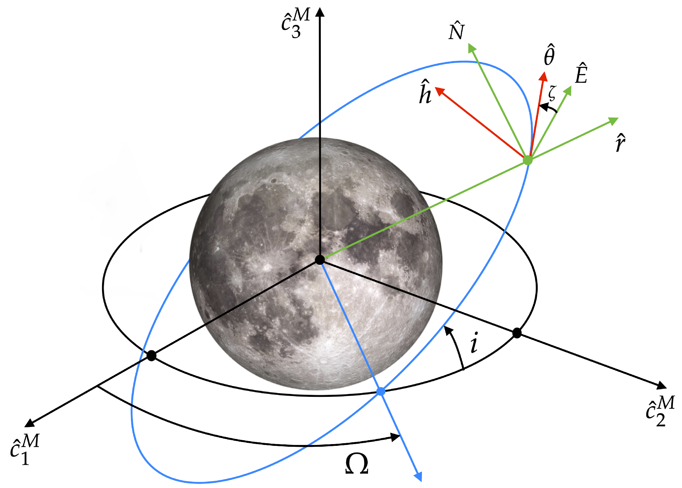
  • The Moon-centered inertial frame (MCI) is identified by unit vectors ( c ^ 1 M , c ^ 2 M , c ^ 3 M ) ; c ^ 1 M and c ^ 2 M are defined as in [23], with the reference epoch set to 17 May 2025; c ^ 3 M points toward the lunar rotation axis.
  • The local-vertical local-horizontal (LVLH) ( r ^ , θ ^ , h ^ ) frame is attached to the center of mass of the spacecraft. The unit vector r ^ is directed from the Moon center to the instantaneous position of the vehicle; h ^ is aligned with the spacecraft’s orbit angular momentum, while θ ^ completes the right-handed set. If Ω denotes the RAAN, i the inclination of the orbital plane, ω the argument of periselenium, and θ the true anomaly, then the following rotations link MCI to the LVLH-frame:
    r ^ θ ^ h ^ = R 3 ( ω + θ ) R 1 ( i ) R 3 ( Ω ) c ^ 1 M c ^ 2 M c ^ 3 M ;
  • The local-horizontal (LH) frame ( r ^ , E ^ , N ^ ) is attached to the center of mass of the spacecraft. The unit vectors E ^ and N ^ are aligned with the local (lunar) east and north directions, respectively. The LH and LVLH frames can be linked through the following relation:
    r ^ θ ^ h ^ = R 1 ( ζ ) r ^ E ^ N ^ ,
    where ζ is the heading angle.
Figure 1 shows the reference frames and the related angles.

2.2. Equations of Motion

A set of modified equinoctial elements x i ( i = 1 , , 6 ) is introduced in order to describe the motion of the spacecraft, which is modeled as a point mass:
x 1 = a ( 1 e 2 ) ,
x 2 = e cos ( Ω + ω ) ,
x 3 = e sin ( Ω + ω ) ,
x 4 = tan i 2 cos Ω ,
x 5 = tan i 2 sin Ω ,
x 6 = Ω + ω + θ ,
where a is the semi-major axis and e the eccentricity. Using the modified equinoctial elements, the dynamical equations are written as
z ˙ = G ( z , x 6 ) a ,
where z = x 1 x 2 x 3 x 4 x 5 T , a = a r a θ a h T is the vector of non-Keplerian accelerations expressed in the LVLH frame, η = 1 + x 2 cos x 6 + x 3 sin x 6 , while
G = x 1 μ 0 2 x 1 η 0 sin x 6 ( 1 + η ) cos x 6 + x 2 η x 4 sin x 6 x 5 cos x 6 η x 3 cos x 6 ( 1 + η ) sin x 6 + x 3 η x 4 sin x 6 x 5 cos x 6 η x 2 0 0 1 + x 4 2 + x 5 2 2 η cos x 6 0 0 1 + x 4 2 + x 5 2 2 η sin x 6 ,
with μ denoting the lunar gravitational parameter. The time derivative for the orbital element x 6 is instead given by
x ˙ 6 = μ x 1 3 η 2 + x 1 μ x 4 sin x 6 x 5 cos x 6 η a h .
The spacecraft is equipped with a chemical high-thrust propulsion system. As the thrusting arcs have very limited duration with respect to the total transfer time, all the maneuvers are modeled using the impulsive thrust approximation.

2.3. Orbit Perturbations

This study addresses the presence of perturbing effects. Other than the lunar gravitational field, which includes several harmonics of the selenopotential, the motion of the spacecraft is affected by the gravitational pull of the Earth and Sun.

2.3.1. Third-Body Perturbations

The gravitational pull of the Earth and Sun can be modeled as third-body perturbations. If r denotes the instantaneous position vector of the spacecraft with respect to the Moon, while r B denotes the vector position of the third body (B) with respect to the Moon, then the perturbing acceleration a 3 B due to a third body can be expressed in the MCI frame, following the Battin–Giorgi approach [24,25]:
a 3 B = μ B r B 3 ( q B + 1 ) 3 / 2 r + r B q B q B 2 + 3 q B + 3 ( q B + 1 ) 3 / 2 + 1 ,
where μ B is the third-body gravitational parameter and
q B : = r · r 2 r · r B r B · r B .
If a 3 E and a 3 S , respectively, denote the third-body accelerations due to the Earth and Sun, then the total perturbing acceleration due to the gravitational pulls of third bodies can be computed as a 3 = a 3 E + a 3 S . Finally, by means of Equation (1), the acceleration is expressed in the LVLH frame. As a matter of fact, if ( a x ( 3 ) , a y ( 3 ) , a z ( 3 ) ) and ( a r ( 3 ) , a θ ( 3 ) , a h ( 3 ) ) , respectively, denote the components of a 3 in the MCI and LVLH frames, then
a r ( 3 ) a θ ( 3 ) a h ( 3 ) = R 3 ( ω + θ ) R 1 ( i ) R 3 ( Ω ) a x ( 3 ) a y ( 3 ) a z ( 3 ) .

2.3.2. Harmonics of the Selenopotential

This research employs the Lunar Prospector LP100K model for the Moon’s gravitational field, which provides the coefficients J l m and λ l m of zonal, tesseral, and sectoral harmonics up to degree 100 [26]. However, only the relevant harmonics are retained in the dynamical model, that is, those associated with coefficients | J l m | > 5 × 10 6 [27]. These coefficients allow expanding the selenopotential U in terms of Legendre polynomials P l , m :
U = μ r { 1 l = 2 R r l J l P l 0 sin ϕ + l = 2 m = 1 l R r l J l , m P l , m sin ϕ cos m ( λ g λ l , m ) } ,
where R is the lunar equatorial radius, ϕ the latitude, and λ g the geographical longitude, taken from the lunar reference meridian. This intersects the line that connects the Earth and Moon at all times and is directed toward the far side of the Moon. The gravitational acceleration can then be obtained in the LH frame:
g = U , where = r ^ r + E ^ r cos ϕ λ g + N ^ r ϕ .
The perturbing acceleration a H is
a H = g + μ r 2 r ^ .
Finally, by means of Equation (2), it is straightforward to obtain the components of the perturbing acceleration in the LVLH frame.

3. Orbital Motion of Gateway

Gateway’s reference orbit is a southern L 2 NRHO. Several criteria were considered in selecting this orbit [28]: (i) an L 2 -family NRHO provides enhanced visibility of the far side of the Moon for communications compared to the L 1 family [17]; (ii) the L 2 NRHOs enjoy more favorable stability properties compared to the L 1 NRHOs, resulting in lower orbit maintenance requirements [29,30]; (iii) a southern NRHO offers lower delta-v and propellant requirements for spacecraft return to Earth’s northern hemisphere; (iv) the southern family also allows very good communications coverage of the lunar south pole, which is a region of high interest for the presence of large water ice deposits in the shadows of craters [31]; and (v) the 9:2 lunar synodic resonance (LSR) with the orbital period of the Moon results in the avoidance of eclipses by the Earth [32]. As a matter of fact, since Earth eclipses can last well beyond current hardware limitations, avoiding them was a primary design goal for this reference orbit. While lunar eclipses are relatively common, with several occurring each year, they always last less than 80 min and pose no threat.
The resulting orbit has a periselenium radius that varies from 3196 to 3557 km, with an average value of 3366 km, and an average orbital period of 6.562 days.

3.1. Gateway Orbit Dynamics from Ephemeris

The ephemeris of Gateway is contained in an SPK-type file, produced by NASA’s Navigation and Ancillary Information Facility (NAIF) [33]. The time span of the ephemeris extends from 2 January 2020 at 08:09:36 UTC to 11 February 2035 at 03:59:59 UTC. The numerical model includes the perturbing effects of the gravitational fields of the Earth, Sun, and Jupiter, as well as the harmonics of the selenopotential up to order and degree 8. This orbit considers small aposelenium maneuvers of a few millimeters per second per revolution, which are needed for stationkeeping purposes. As a matter of fact, the orbit diverges after more than 9 revolutions without maintenance [34]. Figure 2 shows the reference trajectory in the Earth–Moon synodic reference frame. Its inspection reveals a significant impact of the perturbations: the trajectory, which is periodic in the CR3BP, becomes quasi-periodic in the accurate dynamical framework. Therefore, stationkeeping is necessary to maintain the orbit close to the reference one, obtained in CR3BP. The existence of a periodic solution in the CR3BP remains as a quasi-periodic solution even when perturbations are included, in agreement with the Kolmogorov–Arnold–Moser (KAM) theorem [35,36,37]. Indeed, this theorem guarantees the persistence of quasi-periodic motions under small perturbations.

3.2. Gateway Orbit Dynamics from High-Fidelity Model

Gateway’s trajectory can also be reproduced using the high-fidelity model, i.e., by integrating Equation (9). This allows an evaluation of the accuracy of the model and a deeper analysis of the orbital motion of the space station.
The integration is performed using MATLAB 2023b ode113, with both absolute and relative tolerances set to 10 13 . The time frame selected for the integration is slightly longer than the period of the station’s orbit around the Moon, starting on 17 May 2025 at 10:00:00 UTC and ending on 24 May 2025 at 10:00:00 UTC.
Figure 3 displays the relative distance Δ r between the Gateway position obtained by numerical integration in the high-fidelity model and the ephemeris data. The mismatch is mainly due to a different model for the lunar gravity field, which has a large effect around periselenium passages. In addition, the high-fidelity model does not include any aposelenium maneuvers, unlike the ephemeris data.
The high-fidelity model provides insight into the total perturbing acceleration a p , which is shown in Figure 4. Its maximum value corresponds to the aposelenium, which is located at about 3.5 days. Furthermore, the average magnitude ( 3.896 × 10 4 m/s2) is close to the thrust acceleration produced by a low-thrust engine. This confirms that cislunar space is a highly perturbed environment.
Moreover, it is worth pointing out that the osculating RAAN varies by 360 degrees in about 28 days. This behavior is shown in Figure 5.

4. Minimum-Fuel Orbit Transfers (Free RAAN)

This section addresses minimum-fuel two-impulse transfers from Gateway to circular LLOs, thereby minimizing the total change in velocity. Several inclinations of the target LLO are considered, with the RAAN left as a free parameter, in order to identify the most convenient orientation of the orbital plane.

4.1. Formulation of the Problem

The selected target LLO is a circular orbit, with an altitude of h * = 200 km, i.e., with radius r c : = R + h * . Ten equally spaced inclinations are considered in the range [ 0 , 90 ] degrees. Two three-dimensional velocity changes, denoted as Δ V 1 and Δ V 2 , are applied according to the following transfer strategy:
  • Δ V 1 is applied at the initial time t 0 along the orbit of Gateway to inject the spacecraft into a transfer trajectory. Consequently, the spacecraft’s dynamical state after the maneuver is given by
    X 0 + = X 0 ,
    V 0 + = V 0 + Δ V 1 ,
    where ( X 0 , V 0 ) and ( X 0 + , V 0 + ), respectively, indicate the position and velocity vectors before and after the instantaneous application of the velocity change at t 0 ;
  • Δ V 2 is applied at the end of the transfer time to insert the spacecraft into the desired LLO.
The transfer design aims to determine the optimal components of Δ V 1 and the optimal initial time t 0 to start the transfer. The optimization problem is formulated as
min t 0 , Δ V 1 Δ V 1 + Δ V 2
Hence forward, Δ V 1 and Δ V 2 will indicate the magnitudes of the two velocity changes. The method of solution is presented in the following paragraph.

4.2. Method of Solution

As a first step, the desired inclination i d of the final LLO is selected. The problem is solved through numerical optimization, which iteratively performs the following steps:
  • After applying Δ V 1 at t 0 , the spacecraft is inserted into the transfer. Its state is propagated forward in time according to the equations of motion of the high-fidelity model (cfr. Section 2.2), with a maximum ToF of 48 h. The integration ends when the target sphere of radius r c is reached.
  • The value of Ω f for the target orbit can be computed from
    r f · h ^ = 0 ,
    where r f is the spacecraft position vector at the end of the transfer, whose components are expressed in the MCI frame, while
    h ^ = sin Ω f sin i d , cos Ω f sin i d , cos i d c ^ 1 M c ^ 2 M c ^ 3 M
    identifies the direction of the angular momentum associated with the orbit containing the final spacecraft position.
  • Equation (21) yields two solutions for the RAAN, denoted by ( Ω 1 , Ω 2 ). The corresponding values of the argument of latitude ( θ t , 1 , θ t , 2 ) are then calculated. For each solution ( Ω k , θ t , k ), the comparison point P k along the LLO is determined via a single-parameter search, aimed at minimizing the cost function
    J θ t = k r Δ r + k 2 Δ V 2 ,
    where Δ r is the distance of P k from the final position (identified with r f ) , while k r and k 2 are weighting coefficients with proper units. The single parameter of interest is the argument of latitude, identifying P k along the desired final LLO.
  • The primary optimization is conducted using a cost function defined as
    J = c 1 Δ V 1 + c 2 Δ V 2 + c h Δ h , if i d = 90 deg c 1 Δ V 1 + c 2 Δ V 2 + c h Δ h + c r Δ r , if i d < 90 deg
    where Δ h represents the difference between the altitude reached at the end of the transfer and the desired altitude h * , while c 1 , c 2 , c h , and c r are weighting coefficients with proper units. The term Δ h guides the trajectory toward the target sphere. When i d < 90 deg, including Δ r in the cost function yields convergence when the intersection between the transfer and target spheres occurs at latitudes higher than the inclination of the target orbit.
  • The cost function J is evaluated for each pair ( Ω k , θ t , k ) , k = 1 , 2 , and the values that minimize J are selected.
The entire optimization process consists of two consecutive steps:
(i)
A first global optimization of J is performed by means of the Stochastic Fractal Search (SFS) algorithm. Its stochastic approach enhances the exploration phase and reduces the possibility of becoming stuck in local minima. A detailed description of the SFS algorithm is reported in Appendix A.
(ii)
Then, the MATLAB built-in routine fmincon is employed for solution refinement, with an equality constraint on the final altitude, and an inequality constraint on the latitude of r f , i.e., | ϕ ( t f ) | i d . The latter inequality constraint ensures that an LLO with inclination i d passes through r f .
For the numerical simulations, the following canonical units are employed:
  • The distance unit (DU) is equal to the lunar mean equatorial radius,
    DU = 1738 km ;
  • The time unit (TU) is chosen to yield a unit gravitational parameter,
    TU = DU 3 μ ,
    with μ = 4902.8 km3/s2.

4.3. Numerical Results

Figure 6 shows Δ V tot = Δ V 1 + Δ V 2 , with respect to the inclination of the LLO. It is clear that Δ V tot increases as the inclination decreases. This behavior is expected since the osculating inclination remains relatively close to 90 deg. Therefore, transfers to polar or near-polar LLOs require a smaller change in orbital plane and reduced fuel consumption as a result. Table 1 collects the relevant data for the optimal transfers. In particular, the overall velocity change for the final polar LLO is very close to the values found by Bucchioni and Innocenti [21] and Lu et al. [20], who found the values 661 m/s and 650 m/s, respectively. However, the latter works assumed a target LLO similar though not identical to that considered in this work, while using the CR3BP model.
Figure 7 shows the transfer trajectories in the MCI frame for the two limiting cases, i.e., polar and equatorial LLOs. In both cases, the orbital plane of the transfer is close to the orbital plane of the target LLO.

5. Minimum-Fuel Orbit Transfers (Specified RAAN)

The aim of this section is to identify minimum-fuel transfers from Gateway to polar circular LLOs with a maximum ToF of 48 h. Unlike the previous analysis, the RAAN value is no longer a free parameter. Eight scenarios are analyzed, corresponding to different specified RAAN values, evenly distributed in the range [ 0 , 360 ] degrees. Because the osculating RAAN varies by 360 degrees in about 28 days (cf. Figure 5), the transfer starting time is sought in the same interval. Polar orbits are selected as target LLOs because (i) polar inclination requires a lower Δ V tot (cf. Table 1), and (ii) they guarantee the coverage of lunar poles, especially the South pole, which harbors vital water ice deposits [38]. The problem is solved through two different methods, which are described below.

5.1. Formulation of the Problem

The goal is to minimize the total Δ V for a bi-impulsive transfer from Gateway to target LLO. The two velocity changes Δ V 1 and Δ V 2 are applied as with the previous strategy (cf. Section 4.1). The final orbit must not only be circular but also polar, with the specified RAAN value Ω d . The argument of latitude along the target LLO remains a free parameter. The optimization problem can be formulated as
min t 0 , Δ t , θ f Δ V 1 + Δ V 2 .
For this purpose, a metaheuristic method could be directly employed, as in Section 4. However, an alternative two-step approach is here proposed: (i) identifying a preliminary solution through a global optimizer using the Lambert algorithm assuming Keplerian motion (cf. Section 5.2); and (ii) refining the solution through a local optimizer in a high-fidelity dynamical framework (cf. Section 5.2). This method is described in the following paragraph.

5.2. Method 1: Lambert-Based Guess Generation and High-Fidelity Refinement

The initial guess solution is sought through a Lambert problem solving algorithm [39], which allows the determination of the conic connecting two points in three-dimensional space for a given time of flight Δ t . Given the initial and final positions along with a time span, the algorithm efficiently computes the Keplerian transfer trajectory.
In our problem, the initial position and velocity of the spacecraft along the orbit of Gateway are uniquely determined by the designated start time t 0 . The final state at time t f is specified by the argument of latitude θ f of the LLO, whose orientation is fixed by inclination and RAAN.
Therefore, the algorithm requires the following inputs:
  • The initial state ( X 0 , V 0 ) , identified by t 0 ;
  • The final state ( X f , V f ) , identified by θ f ;
  • The transfer time, Δ t = t f t 0 .
Both state vectors are referenced in the MCI frame. The algorithm outputs the orbit elements of the transfer trajectory, allowing the determination of Δ V 1 and Δ V 2 for Gateway-to-transfer orbit insertion at t 0 and for transfer orbit-to-LLO insertion at t f .
The optimization problem, as formulated in Equation (27), is solved by means of the SFS, with the two velocity changes determined by the Lambert algorithm. Its introduction is motivated by the immediate determination of the transfer trajectory within a Keplerian framework. Consequently, propagation becomes unnecessary when SFS is used for optimization, making the search for a solution more efficient.
The initial guess, which solves the problem (27) in a Keplerian model, is employed to refine the solution within the high-fidelity framework (cf. Section 2.3). This refinement involves solving the optimization problem (20) through MATLAB fmincon.
While the guess value t 0 is directly obtained from the global optimization procedure, the three components of Δ V 1 in the MCI frame are computed through the Lambert algorithm, starting from the previous optimal solution. The optimization process advances by propagating the perturbed motion of the spacecraft using Equation (9) after the impulsive application of Δ V 1 . Due to the non-Keplerian dynamical environment, reaching the final position at θ f within Δ t is unlikely. Consequently, the propagation is stopped when an altitude of 200 km is reached or at the periselenium of the transfer orbit. Finally, Δ V 2 is applied. This method ensures targeting a circular and polar orbit, although it may not meet the prescribed RAAN condition. Therefore, within fmincon, the difference between the final and the desired RAAN is enforced as a nonlinear constraint.

5.3. Numerical Results Using Method 1

As a first step, the SFS algorithm is employed to obtain the initial guess as a solution of the Keplerian Lambert problem. The tuning parameters are set as follows:
  • Population size, 50;
  • Maximum generation number, 250;
  • Maximum diffusion number, 10.
Table 2 collects the results of the guess generation based on the Lambert algorithm.
From inspection of Table 2, it is evident that most trajectories yield the maximum ToF (48 h), corresponding to the upper bound of the search interval, as a result of the optimization process.
Secondly, the fmincon routine is employed to refine the solution in the high-fidelity model, while enforcing the nonlinear constraint on the final RAAN:
1 cos ( Ω d Ω f ) 1.5 · 10 6 .
This tolerance yields an error on the final RAAN less than 0.1 deg. The search space is identified by lower and upper bounds on the variation of the initial guess time t 0 ( G ) ( [ t 0 ( G ) δ t 0 , t 0 ( G ) + δ t 0 ] ), as well as on the Δ V 1 components along the LVLH frame (respectively, adding ± δ V r , ± δ V θ , ± δ V h ), where δ t 0 = 1 h, δ V r δ V θ δ V h = 50 m/s. However, a further reduction in the search space was necessary in order to guarantee convergence for the cases associated with Ω d = 270 , 315 deg. Table 3 collects the results of the solution refinement. The algorithm is capable of generating feasible transfers that satisfy the requirements on the final orbit.
Figure 8 shows the stream of trajectories associated with different RAAN values of the target LLO. Interestingly, the trajectories associated with the lowest Δ V tot , e.g., Ω d = 90 or 270 deg (cf. Table 3) exhibit a reduced change in direction after the first velocity change; instead, the greatest values of Δ V tot are associated with a significant change in orbital plane. Moreover, orbit injection always occurs in the north hemisphere.

5.4. Method 2: High-Fidelity Heuristic Guess and Local Refinement

The heuristic algorithm (cf. Section 4) is here exploited to obtain the global optimal parameters for the sake of comparison. However, as Ω f is fixed, there is no need to solve Equation (22). Thus, a single value is determined for θ t and for the cost function. The SFS algorithm is initially set to the same parameters as in Section 5.3. However, as the cost function exhibits several local minima, some scenarios required several attempts and an appropriate tuning of the parameters in order to increase the exploration capabilities of the algorithm. The weighting coefficients k 1 , k 2 and c 1 , c 2 , c r , c h (cf. Section 4.2) are set to unit values. As illustrated in Section 4.2, the solution of global optimization is refined by means of fmincon.

5.5. Numerical Results Using Method 2

Table 4 collects the outcomes of the optimization process based on high-fidelity heuristic guess generation and subsequent local refinement.

5.6. Comparison of Results

Figure 9 shows a comparison between the two strategies for each scenario. Remarkably, both approaches yield very close results in terms of Δ V tot . A close inspection of Table 3 and Table 4 highlights that, even though the starting times may be different, they provide similar Δ V tot . In particular, the Lambert algorithm is capable of providing a good initial guess solution, though in a Keplerian dynamical framework. As a matter of fact, the semi-analytical approach is proven to guarantee a faster convergence with respect to the heuristic method, as the global exploration does not require the integration of the high-fidelity equations of motion. As an example, a single iteration of the SFS algorithm on a 48-core computer requires on average 1.58 s for the Lambert-based guess generation and 67.17 s for the heuristic optimization. On the other hand, the accuracy of the Lambert-based guess solution is expected to decrease when trajectories associated with longer transfer times are sought, because of the action of perturbations.

6. Concluding Remarks

This research addresses minimum-fuel orbit transfers from Gateway to LLOs associated with a maximum duration of 48 h. The spacecraft is equipped with a chemical engine. The dynamical framework includes all relevant gravitational perturbations, including third-body effects of the Earth and Sun. Two different cases are explored: first, a global optimization technique based on a heuristic algorithm is developed to obtain the optimal transfer toward an LLO with free RAAN. Several scenarios are investigated, associated with different inclinations of the target orbit; the numerical results prove that the algorithm is capable of identifying the optimal transfer leading to the desired orbit. Unsurprisingly, polar target orbits are reached with lower fuel expenditure. Then, a semi-analytical approach is developed, aimed at achieving the optimal minimum-fuel transfer toward a polar target orbit with specified RAAN. This strategy relies on a numerical solver based on the Lambert theorem, which provides an initial guess. This solution is then refined by local numerical optimization in the high-fidelity dynamical framework. The results attained with this semi-analytical approach are shown to be very similar (in most cases) to those found with high-fidelity heuristic guess generation. The latter approach, however, turns out to be much more computationally expensive.

Author Contributions

Conceptualization, E.M.L., D.S., G.D.A. and M.P.; methodology, E.M.L., D.S. and M.P.; software, E.M.L. and D.S.; validation, G.D.A. and M.P.; formal analysis, E.M.L., D.S. and G.D.A.; investigation, E.M.L. and D.S.; resources, M.P.; data curation, G.D.A. and M.P.; writing—original draft preparation, E.M.L., D.S. and G.D.A.; writing—review and editing, M.P.; visualization, E.M.L., D.S. and G.D.A.; supervision, M.P.; project administration, M.P. All authors have read and agreed to the published version of the manuscript.

Funding

This research received no external funding.

Institutional Review Board Statement

Not applicable.

Informed Consent Statement

Not applicable.

Data Availability Statement

Data reported in the article.

Acknowledgments

Dario Sanna acknowledges Nico Sanna of University of Tuscia, who kindly provided the access to DIBAF department of advanced computing resources, which allowed reduction of computational runtime, with reference to the high-fidelity heuristic optimization. The authors also express their gratitude to Francesco Corallo, for his help with the heuristic solution methodology.

Conflicts of Interest

The authors declare no conflicts of interest.

Abbreviations

The following abbreviations are used in this manuscript:
CR3BPCircular restricted 3-body problem
DRODistant retrograde orbit
LEOLow earth orbit
LHLocal horizontal
LLOLow lunar orbit
LVLHLocal vertical local horizontal
MCIMoon-centered inertial
NRHONear-rectilinear halo orbit
RAANRight ascension of the ascending node
SFSStochastic fractal search
ToFTime of flight

Appendix A. Stochastic Fractal Search Algorithm

The Stochastic Fractal Search (SFS) technique was first introduced by H. Salimi in 2015 [40]. It is a heuristic technique aimed at finding the optimal parameter set that minimizes a specified fitness function. The algorithm at hand is inspired by the natural phenomenon of growth, based on the mathematical concept of fractals, to enhance both convergence and accuracy of the numerical search process. This method was proven to exhibit remarkable capabilities of efficient exploration of the search space (diversification) and improvement of promising solutions (intensification).
SFS evolves a population of individuals. Each of them is associated with a parameter vector at a given iteration and includes the values of the unknown parameters of the problem. Each individual (i.e., parameter vector) represents a possible solution to the problem, and corresponds to a specific value of the fitness function. The initial population is randomly generated. At the end of the process, the best parameter vector (i.e., the one that minimizes the fitness function) is selected. The central idea of SFS consists in generating individuals for the next generation through:
  • An initial diffusing phase, in which the existing individuals are “diffused” around their current position. To generate the branch-like fractal shape, the diffusion-limited aggregation (DLA) [41] model is employed, by exploiting the Gaussian walk statistical technique. Only the best individual generated from this diffusion is considered, while the others are discarded in order to avoid a dramatic increase in the number of individuals.
  • A subsequent updating phase, in which the less well performing candidates are replaced by other individuals, randomly generated. This updating step aims at introducing a way for the individuals to exchange information, to speed up convergence toward the optimal solution.
Unconstrained parameter optimization problems can be stated as follows: determine the optimal values of the n unknown parameters χ 1 , , χ n such that the fitness function J is minimized. The time evolution of the dynamical system under consideration depends on χ 1 , , χ n , which are constrained to their respective ranges,
a k χ k b k ( k = 1 , , n ) .
SFS evolves a population of N individuals. Each of them, associated with index i ( i = 1 , , N ) , includes the values of the n unknown parameters of the problem,
χ ( i ) = χ 1 ( i ) χ n ( i ) T .
The initial population of SFS is randomly generated by introducing N individuals, whose parameters are (stochastically) uniformly distributed in the respective search spaces, defined by Equation (A1). The steps that follow comprise the generic iteration (denoted with index g), which leads to generating a new populations of individuals.
  • For i = 1 , , N , evaluate the fitness function associated with individual i, J ˜ i ( g ) = J ˜ ( χ ( g ) ( i ) ) .
  • The best individual, which corresponds to the current minimum value of the fitness function, is identified and is associated with index i o p t .
  • Diffusion phase. For i = 1 , , N :
    (a)
    The “diffusion limited aggregation” growth process employs the Gaussian distribution to generate new individuals; N D is the number of individuals generated by diffusion of individual i. For j = 1 , , N D ,
    Y ( i , j ) = g ( μ opt , σ ) + ( ε χ ( g ) ( i opt ) ε χ ( g ) ( i ) ) if ε < P G W g ( μ i , σ ) if ε P G W ,
    where i o p t = arg min i = 1 , , N J ˜ i ( g ) , P G W denotes a threshold value, whereas ε , ε , and ε are three random variables with uniform distribution in [ 0 , 1 ] . Symbol g ( μ , σ ) denotes a vector with random components g k , subject to Gaussian distribution, with mean value μ k (component of μ ) and standard deviation
    σ = log g g χ ( g ) ( i ) χ ( g ) ( i opt ) ,
    The term log g / g aims at decreasing the size of the Gaussian jumps, to promote more localized search as the generation index g increases.
    (b)
    The bounds (A1) are enforced for each component Y k ( i , j ) ( k = 1 , , n ) of the N D generated individuals. For j = 1 , , N D and k = 1 , , n ,
    if Y k ( i , j ) < a k Y k ( i , j ) = a k if Y k ( i , j ) > b k Y k ( i , j ) = b k ;
    (c)
    For j = 1 , , N D , evaluate the fitness function associated with individual Y ( i , j ) .
    (d)
    Select the best individual Y ¯ ( i ) = Y ( i , l ) among { Y ( i , j ) } j = 1 , , N D , such that J ˜ Y ¯ ( i ) J ˜ Y ( i , j ) j .
    (e)
    Select the best individual between Y ¯ ( i ) and χ ( g ) ( i ) , i.e.,
    χ ( i ) = Y ¯ ( i ) if J ˜ χ ( g ) ( i ) > J ˜ Y ¯ ( i ) χ ( g ) ( i ) if J ˜ χ ( g ) ( i ) J ˜ Y ¯ ( i ) .
    At the end of the diffusion phase, N individuals χ ( g ) ( i ) are replaced by N individuals χ ( i ) .
  • For i = 1 , , N , evaluate the fitness function J ˜ χ ( i ) .
  • First updating phase. For i = 1 , , N :
    (a)
    A probability value P a ( i ) is assigned to each individual, in order to give a higher probability to survive to more performing individuals:
    P a ( i ) = 1 rank ( i ) N ,
    where rank ( i ) equals 1 for the best individual and N for the worst one.
    (b)
    For k = 1 , , n , select two random integers ( m , r ) in the interval [ 1 , N ] and set
    Y k ( i ) = χ k ( r ) ε χ k ( m ) χ k ( i ) if P a ( i ) ε χ k ( i ) if P a ( i ) > ε ,
    where ε is a random number with a uniform distribution in [ 0 , 1 ] . In this way, a “mutant” vector Y ( i ) is generated.
    (c)
    For k = 1 , , n ,
    if Y k ( i , j ) < a k Y k ( i , j ) = a k if Y k ( i , j ) > b k Y k ( i , j ) = b k ;
    (d)
    Evaluate the fitness function associated with individual Y ( i ) .
    (e)
    Select the best individual between Y ( i ) and χ ( i ) , i.e.,
    χ ( i ) = Y ( i ) if J ˜ χ ( i ) > J ˜ Y ( i ) χ ( i ) if J ˜ χ ( i ) J ˜ ( Y ( i ) ) .
    At the end of the first updating phase, N individuals χ ( i ) are replaced by N individuals χ ( i ) .
  • For i = 1 , , N , evaluate the fitness function J ˜ χ ( i ) .
  • Second updating phase. For i = 1 , , N :
    (a)
    A probability value P a ( i ) is assigned again to each individual, using the preceding definition of P a ( i ) .
    (b)
    For k = 1 , , n , select two random integers ( m , r ) in the interval [ 1 , N ] and set
    Y ( i ) = χ ( i ) ε ^ χ ( r ) χ ( i o p t ) if ε ^ 0.5 and P a ( i ) ε χ ( i ) ε ^ ( χ ( r ) χ ( m ) ) if ε ^ > 0.5 and P a ( i ) ε χ ( i ) if P a ( i ) > ε ,
    where ε and ε ^ are two random numbers with uniform distribution in [ 0 , 1 ] . In this way a new “mutant” vector Y ( i ) is generated.
    (c)
    For k = 1 , , n ,
    if Y k ( i , j ) < a k Y k ( i , j ) = a k if Y k ( i , j ) > b k Y k ( i , j ) = b k ;
    (d)
    Evaluate the fitness function associated with individual Y ( i ) .
    (e)
    Select the best individual between Y ( i ) and χ ( i ) , i.e.,
    χ ( g + 1 ) ( i ) = Y ( i ) if J ˜ χ ( i ) > J ˜ Y ( i ) χ ( i ) if J ˜ χ ( i ) J ˜ Y ( i ) .
    At the end of the second updating phase, the new population is generated.
At the end of the process, the parameter vector associated with the best individual is expected to contain the optimal values of the unknown parameters, which correspond to the global minimum of J ˜ . The algorithm stops when the termination criterion is met, e.g., if the fitness function has reached a sufficiently low value or after a specified (large) number of generations.

References

  1. NASA. Artemis Plan. 2020. Available online: https://www.nasa.gov/wp-content/uploads/2020/12/artemis_plan-20200921.pdf (accessed on 3 July 2023).
  2. NASA. What Is CAPSTONE? Available online: https://www.nasa.gov/smallspacecraft/capstone/ (accessed on 12 July 2023).
  3. Howell, K.C.; Kakoi, M. Transfers between the Earth–Moon and Sun–Earth systems using manifolds and transit orbits. Acta Astronaut. 2006, 59, 367–380. [Google Scholar] [CrossRef]
  4. Alessi, E.M.; Gomez, G.; Masdemont, J.J. Two-manoeuvres transfers between LEOs and Lissajous orbits in the Earth–Moon system. Adv. Space Res. 2010, 45, 1276–1291. [Google Scholar] [CrossRef]
  5. Pontani, M.; Teofilatto, P. Polyhedral representation of invariant manifolds applied to orbit transfers in the Earth–Moon system. Acta Astronaut. 2016, 119, 218–232. [Google Scholar] [CrossRef]
  6. Patrick, B.; Pascarella, A.; Woollands, R. Hybrid Optimization of High-Fidelity Low-Thrust Transfers to the Lunar Gateway. J. Astronaut. Sci. 2023, 70, 27. [Google Scholar] [CrossRef]
  7. Singh, S.K.; Anderson, B.D.; Taheri, E.; Junkins, J.L. Low-thrust transfers to southern L2 near-rectilinear halo orbits facilitated by invariant manifolds. J. Optim. Theory Appl. 2021, 191, 517–544. [Google Scholar] [CrossRef]
  8. He, G.; Conte, D.; Melton, R.G.; Spencer, D.B. Fireworks Algorithm Applied to Trajectory Design for Earth to Lunar Halo Orbits. J. Spacecr. Rocket. 2020, 57, 235–246. [Google Scholar] [CrossRef]
  9. Muralidharan, V.; Howell, K.C. Stretching directions in cislunar space: Applications for departures and transfer design. Astrodynamics 2023, 7, 153–178. [Google Scholar] [CrossRef]
  10. Parrish, N.L.; Parker, J.S.; Hughes, S.P.; Heiligers, J. Low-thrust transfers from distant retrograde orbits to L2 halo orbits in the Earth-Moon system. In Proceedings of the International Conference on Astrodynamics Tools and Techniques, Darmstadt, Germany, 14–17 March 2016. [Google Scholar]
  11. Pino, B.P.; Howell, K.C.; Folta, D. An energy-informed adaptive algorithm for low-thrust spacecraft cislunar trajectory design. In Proceedings of the AAS/AIAA Astrodynamics Specialist Conference, South Lake Tahoe, CA, USA, 9–13 August 2020. [Google Scholar]
  12. Pritchett, R.E. Strategies for Low-Thrust Transfer Design Based on Direct Collocation Techniques. Ph.D. Thesis, Purdue University, West Lafayette, IN, USA, 2020. [Google Scholar]
  13. Das-Stuart, A.; Howell, K.C.; Folta, D.C. Rapid trajectory design in complex environments enabled by reinforcement learning and graph search strategies. Acta Astronaut. 2020, 171, 172–195. [Google Scholar] [CrossRef]
  14. McCarty, S.L.; Burke, L.M.; McGuire, M. Parallel monotonic basin hopping for low thrust trajectory optimization. In Proceedings of the 2018 Space Flight Mechanics Meeting, Kissimmee, FL, USA, 8–12 January 2018; p. 1452. [Google Scholar]
  15. Vutukuri, S. Spacecraft Trajectory Design Techniques Using Resonant Orbits. Master’s Thesis, Purdue University, West Lafayette, IN, USA, 2018. [Google Scholar]
  16. Zimovan-Spreen, E.M.; Howell, K.C. Dynamical structures nearby NRHOS with applications in cislunar space. In Proceedings of the AAS/AIAA Astrodynamics Specialist Conference, Portland, ME, USA, 11–15 August 2019; p. 18. [Google Scholar]
  17. Whitley, R.; Martinez, R. Options for staging orbits in cislunar space. In Proceedings of the 2016 IEEE Aerospace Conference, Big Sky, MT, USA, 5–12 March 2016; pp. 1–9. [Google Scholar]
  18. Trofimov, S.; Shirobokov, M.; Tselousova, A.; Ovchinnikov, M. Transfers from near-rectilinear halo orbits to low-perilune orbits and the Moon’s surface. Acta Astronaut. 2020, 167, 260–271. [Google Scholar] [CrossRef]
  19. Rozek, M.; Ogawa, H.; Ueda, S.; Ikenaga, T. Multi-objective optimisation of NRHO-LLO orbit transfer via surrogate-assisted evolutionary algorithms. In Proceedings of the 27th International Symposium on Space Flight Dynamics, Melbourne, Australia, 24–28 February 2019. [Google Scholar]
  20. Lu, L.; Li, H.; Zhou, W.; Liu, J. Design and analysis of a direct transfer trajectory from a near rectilinear halo orbit to a low lunar orbit. Adv. Space Res. 2021, 67, 1143–1154. [Google Scholar] [CrossRef]
  21. Bucchioni, G.; Innocenti, M. Phasing maneuver analysis from a low lunar orbit to a near rectilinear halo orbit. Aerospace 2021, 8, 70. [Google Scholar] [CrossRef]
  22. Zeng, H.; Li, Z.; Xu, R.; Peng, K.; Wang, P. Further Advances for staging orbits of manned lunar exploration mission. Acta Astronaut. 2023, 204, 281–293. [Google Scholar] [CrossRef]
  23. Pontani, M.; Di Roberto, R.; Graziani, F. Lunar orbit dynamics and maneuvers for Lunisat missions. Acta Astronaut. 2018, 149, 111–122. [Google Scholar] [CrossRef]
  24. Battin, R.H. An Introduction to the Mathematics and Methods of Astrodynamics; AIAA: Reston, VA, USA, 1999. [Google Scholar]
  25. Giorgi, S. Una Formulazione Caratteristica del Metodo Encke in Vista dell’Applicazione Numerica; Università di Roma, Scuola di Ingegneria Aerospaziale: Roma, Italy, 1964. [Google Scholar]
  26. Konopliv, A.; Asmar, S.; Carranza, E.; Sjogren, W.; Yuan, D. Recent gravity models as a result of the Lunar Prospector mission. Icarus 2001, 150, 1–18. [Google Scholar] [CrossRef]
  27. Leonardi, E.M.; Pontani, M.; Carletta, S.; Teofilatto, P. Low-Thrust Nonlinear Orbit Control for Very Low Lunar Orbits. Appl. Sci. 2024, 14, 1924. [Google Scholar] [CrossRef]
  28. Lee, D.E. White Paper: Gateway Destination Orbit Model: A Continuous 15 Year NRHO Reference Trajectory; Technical Report; NASA Johnson Space Center: Houston, TX, USA, 2019.
  29. Davis, D.; Bhatt, S.; Howell, K.; Jang, J.W.; Whitley, R.; Clark, F.; Guzzetti, D.; Zimovan, E.; Barton, G. Orbit maintenance and navigation of human spacecraft at cislunar near rectilinear halo orbits. In Proceedings of the AAS/AIAA Space Flight Mechanics Meeting, San Antonio, TX, USA, 5–9 February 2017. [Google Scholar]
  30. Davis, D.C.; Phillips, S.M.; Howell, K.C.; Vutukuri, S.; McCarthy, B.P. Stationkeeping and transfer trajectory design for spacecraft in cislunar space. In Proceedings of the AAS/AIAA Astrodynamics Specialist Conference, Columbia River Gorge, Stevenson, WA, USA, 20–24 August 2017; Springer Nature: London, UK, 2017; Volume 8. [Google Scholar]
  31. Li, S.; Lucey, P.G.; Milliken, R.E.; Hayne, P.O.; Fisher, E.; Williams, J.P.; Hurley, D.M.; Elphic, R.C. Direct evidence of surface exposed water ice in the lunar polar regions. Proc. Natl. Acad. Sci. USA 2018, 115, 8907–8912. [Google Scholar] [CrossRef]
  32. McGuire, M. Power & Propulsion Element (PPE) Spacecraft Reference Trajectory Document; Vol. PPE-DOC-0079, Rev B; NASA, John H. Glenn Research Center: Cleveland, OH, USA, 2018; pp. 4–5.
  33. Lee, D.E.; Whitley, R.J.; Acton, C. Sample Deep Space Gateway Orbit. 2018. Available online: https://naif.jpl.nasa.gov/pub/naif/misc/MORE_PROJECTS/DSG/ (accessed on 7 July 2023).
  34. Zimovan-Spreen, E.M.; Davis, D.C.; Howell, K.C. Recovery Traejctories for Inadvertent Departures from an NRHO. In Proceedings of the AAS/AIAA Spaceflight Mechanics Meeting, Virtual Event, 1–3 February 2021. paper AAS 21-345. [Google Scholar]
  35. Kolmogorov, A.N. On the Conservation of Conditionally Periodic Motions under Small Perturbation of the Hamiltonian. Dokl. Akad. Nauk SSSR 1954, 98, 527–530. [Google Scholar]
  36. Arnol’d, V.I. Proof of a theorem of A. N. Kolmogorov on the invariance of quasi-periodic motions under small perturbations of the Hamiltonian. Uspekhi Mat. Nauk 1963, 18, 9–36. [Google Scholar] [CrossRef]
  37. Moser, J. On invariant curves of area-preserving mappings of an annulus. Matematika 1962, 6, 51–68. [Google Scholar]
  38. JPL. Ice Confirmed at the Moon’s Poles. 2018. Available online: https://www.jpl.nasa.gov/news/ice-confirmed-at-the-moons-poles (accessed on 12 July 2023).
  39. Curtis, H.D. Orbital Mechanics for Engineering Students; Butterworth-Heinemann: Oxford, UK, 2013. [Google Scholar]
  40. Salimi, H. Stochastic Fractal Search: A powerful metaheuristic algorithm. Knowl. Based Syst. 2015, 75, 1–18. [Google Scholar] [CrossRef]
  41. Witten, T.A.; Sander, L.M. Diffusion-limited aggregation. Phys. Rev. B 1983, 27, 5686–5697. [Google Scholar] [CrossRef]
Figure 1. MCI, LVLH, and LH frames.
Aerospace 11 00460 g001
Figure 2. Gateway trajectory in the Earth–Moon synodic reference frame, for ten periods.
Aerospace 11 00460 g002
Figure 3. Norm of Gateway position difference between high-fidelity model and ephemeris data for seven days.
Aerospace 11 00460 g003
Figure 4. Norm of the total perturbing acceleration acting on Gateway for seven days.
Aerospace 11 00460 g004
Figure 5. Time history of the RAAN in 28 days.
Aerospace 11 00460 g005
Figure 6. Δ V tot as a function of LLO inclination.
Aerospace 11 00460 g006
Figure 7. Transfers from Gateway NRHO toward an LLO, in the MCI frame.
Aerospace 11 00460 g007
Figure 8. Stream of trajectories associated with different RAAN of the target orbit (with zoom on the injection positions in the inset). The trajectory of Gateway is depicted with a dashed black line.
Aerospace 11 00460 g008
Figure 9. Comparison between Δ V tot for different values of RAAN.
Aerospace 11 00460 g009
Table 1. Values of Δ V tot , starting epoch, and ToF according to the inclination of the LLO.
i [deg] Δ V tot [m/s] t 0 (UTC)ToF [h]
9066622 May 2025 at 09:4436.13
8071022 May 2025 at 19:0527.15
7077023 May 2025 at 03:3718.95
6084817 May 2025 at 16:3547.96
5090817 May 2025 at 17:1048.00
40100117 May 2025 at 14:4644.78
30111517 May 2025 at 13:3241.20
20125317 May 2025 at 12:3221.95
10139517 May 2025 at 11:5712.41
0154117 May 2025 at 11:328.33
Table 2. Initial guess solutions obtained through Lambert algorithm.
Ω d Δ V 1 Δ V 2 Δ V tot t 0 ToF
[deg] [m/s] [m/s] [m/s] (UTC) [h]
09064873830 May 2025 at 00:215.05
4515269084227 May 2025 at 15:5248.00
90406336735 June 2025 at 02:5917.86
13520265585721 May 2025 at 01:0648.00
1804567672110 June 2025 at 13:0148.00
22519765485127 May 2025 at 09:5148.00
2704763568223 May 2025 at 09:0413.15
31517567885321 May 2025 at 05:1448.00
Table 3. Results of solution refinement using fmincon.
Ω d | Ω f Ω d | Δ V 1 Δ V 2 Δ V tot t 0 ToF
[deg] [deg] [m/s] [m/s] [m/s] (UTC) [h]
08.8 × 10 5 9064873829 May 2025 at 01:355.04
459.0 × 10 5 12071883827 May 2025 at 15:2347.99
901.2 × 10 2 386346725 June 2025 at 02:3018.24
1351.4 × 10 5 18865884621 May 2025 at 01:0447.98
1802.9 × 10 4 2971674510 June 2025 at 12:3047.57
2258.4 × 10 4 18265784027 May 2025 at 09:4548.00
2701.7 × 10 3 4663668223 May 2025 at 08:4513.43
3153.0 × 10 4 15269985121 May 2025 at 04:5947.10
Table 4. Refined results of heuristic global optimization.
Ω d | Ω f Ω d | Δ V 1 Δ V 2 Δ V tot t 0 ToF
[deg] [deg] [m/s] [m/s] [m/s] (UTC) [h]
05.9 × 10 5 7866173929 May 2025 at 23:176.05
453.2 × 10 10 16766783427 May 2025 at 07:4248.00
901.2 × 10 4 346376714 June 2025 at 22:4521.90
1355.9 × 10 3 18765984621 May 2025 at 01:1648.00
1803.1 × 10 6 3171274310 June 2025 at 11:2648.00
2252.6 × 10 10 18465684027 May 2025 at 09:2548.00
2707.1 × 10 5 4363968223 May 2025 at 07:1714.85
3154.6 × 10 7 17566684120 May 2025 at 23:3748.00
Disclaimer/Publisher’s Note: The statements, opinions and data contained in all publications are solely those of the individual author(s) and contributor(s) and not of MDPI and/or the editor(s). MDPI and/or the editor(s) disclaim responsibility for any injury to people or property resulting from any ideas, methods, instructions or products referred to in the content.

