Effects of Leading Edge Radius on Stall Characteristics of Rotor Airfoil

Abstract

The effects of leading edge radius on the static and dynamic stall characteristics of rotor airfoils are investigated. Initially, a parametric airfoil (PARFOIL) method is employed to generate four morphed airfoils with different leading edge radii based on a NACA 0012 airfoil. Subsequently, the Reynolds-averaged Navier–Stokes (RANS) method is employed to simulate the aerodynamic characteristics of static airfoils, while the improved delayed detached-eddy simulation (IDDES) method is employed for pitching airfoils. The effectiveness and accuracy of the computational fluid dynamics (CFD) methods are demonstrated through favorable agreement between the numerical and experimental results. Finally, both the static and dynamic aerodynamic characteristics are simulated and analyzed for the airfoils with varying leading edge radii. Comparative analyses indicate that at low Mach numbers, the high adverse pressure gradient near the leading edge is the primary cause of leading edge separation and stall. A larger leading edge radius helps to reduce the suction pressure peak and adverse pressure gradients, thus delaying the leading edge separation and stall of airfoil. At high Mach numbers, the leading edge separation and stall are mainly induced by the shock wave. Variations in leading edge radius have minimal impacts on the high adverse pressure gradient induced by the shock wave, thus making the stall characteristics of airfoils almost unaffected at high Mach numbers.

1. Introduction

The static and dynamic stalls of rotor airfoils are the main factors that limit the aerodynamic performance of helicopters. The static stall primarily affects the hover performance, while the dynamic stall affects the forward and maneuvering performance. For this reason, airfoil stall and its control have received a great deal of research attention.

Based on the features of pre-stall boundary layer separation, the stall of airfoils is categorized into various types. The static stall of airfoils generally falls into three categories: thin-airfoil stall, leading edge stall, and trailing edge stall [1]. In contrast, the dynamic stall of airfoils is categorized into four types: thin airfoil stall, trailing edge stall, leading edge stall, and mixed stall [2,3,4]. Helicopter rotor airfoils generally encounter the latter three stall types at low to moderate Mach numbers. Typically, thicker airfoils are prone to trailing edge stall, while thinner airfoils tend to experience leading edge stall. At high Mach numbers, rotor airfoils might undergo shock-induced stall.

The stall characteristics of rotor airfoils are influenced by various factors, including compressibility [5,6,7,8,9], Reynolds number [5,10,11,12], reduced frequency [13,14], maximum angle of attack (AoA), and airfoil geometry [2,12,15,16,17,18,19]. Many studies have examined the corresponding influence mechanism of these parameters, which helps to further control the airfoil stall. The methods for controlling stall of rotor airfoils can be divided into two main categories: active methods and passive methods. The former includes suction/blow [20,21], synthetic jets [22], variable droop leading edges [23,24], and trailing edge flaps [25]. These active methods face challenges in engineering applications. Airfoil design, being a passive method, is currently considered practical and effective for alleviating stall. The airfoil geometry is either morphed or designed to meet the specific requirements of helicopters. Extensive research has been conducted to explore the influence of airfoil geometry on aerodynamic stall characteristics.

McCroskey et al. [15,16,17] measured both the static and dynamic aerodynamic characteristics of multiple airfoil profiles, such as NACA 0012, SC1095, and VR-7. The experimental results have indicated that all of the airfoils tested present significant advantages compared to the standard NACA 0012 airfoil. This suggests that the aerodynamic characteristics of an airfoil are significantly influenced by its shape. The experiment was conducted at a Mach number less than or equal to 0.3, without considering the conditions at higher Mach numbers.

Zhu et al. [12] conducted experimental measurements on VR-7 and VR-12 airfoils at a Reynolds number ranging from 0.2 × 10⁶ to 1 × 10⁶. The results indicate that airfoil geometry influences the sensitivity toward the Reynolds number in dynamic stall, which is consistent with the conclusions of Noonan and Bingham [5]. These demonstrate that the effects of airfoil geometry and incoming flow parameters on airfoil stall characteristics are not independent of each other.

Sharma and Visbal [18] conducted a study to examine the impact of airfoil thickness on both static and dynamic stall onset by employing large eddy simulation (LES) method. The study simulated and analyzes the aerodynamic characteristics of four symmetric NACA airfoils of varying thickness at a Mach number of 0.1 and Reynolds number of 2 × 10⁵. The numerical results indicate that thinner airfoils experience leading edge stall triggered by the burst of an LSB, whereas thicker airfoils experience trailing edge stall due to the interaction between trailing edge separation (TES) and the LSB. It should be noted that the freestream Mach number and Reynolds number studied in this research are inconsistent with the typical operating conditions of helicopter rotor airfoils.

Shum and Lee [19] carried out a numerical study to investigate the effect of airfoil design parameters on deep dynamic stall loads. Multiple parameters were considered, such as camber, thickness, thickness crest position, leading edge radius, trailing edge camber, and boat-tail angle. To evaluate the relative influence of these parameters, the researchers employed Morris’s method. The numerical results indicated that all of the design parameters have a noticeable influence on the aerodynamic loads of airfoil and the leading edge radius has the greatest variation for lift coefficient. Tang et al. [26], Wang et al. [27] and Jing et al. [28] conducted an unsteady aerodynamic optimization of an airfoil. The results indicate that increasing the leading edge radius has positive effects on the aerodynamic stall characteristics of the airfoil. However, they only considered conditions at low or medium Mach numbers and neglected the underlying mechanism.

McCroskey et al. [2] measured the aerodynamic characteristics of several morphed airfoils by varying the leading edge geometry of a NACA 0012 airfoil. The experimental results showed that the airfoil with a sharp leading edge exhibits a stronger leading edge stall than the baseline NACA 0012 airfoil. Due to the limitations of the test conditions, the incoming flow velocity is only 30.5 m/s.

Overall, airfoil geometry, particularly the leading edge radius, has a significant impact on the stall characteristics of rotor airfoils. However, the majority of the study focuses on the effects on aerodynamic loads at low Mach numbers without thoroughly exploring the underlying mechanisms. It remains unclear how the leading edge radius affects stall at high Mach numbers. To address this, comprehensive research is conducted to examine the effects of leading edge radius on the stall characteristics of rotor airfoils at both low and high Mach numbers. The aim is to reveal the influencing mechanisms that contribute to airfoil stall control. In this paper, a method for parametrizing airfoil geometry is first introduced. Subsequently, the CFD method used for airfoil simulations and its validation are described. Then, the aerodynamic stall characteristics of airfoils with different leading edge radii are discussed comprehensively. Lastly, the research findings are presented in the form of conclusions.

2. Numerical Methods

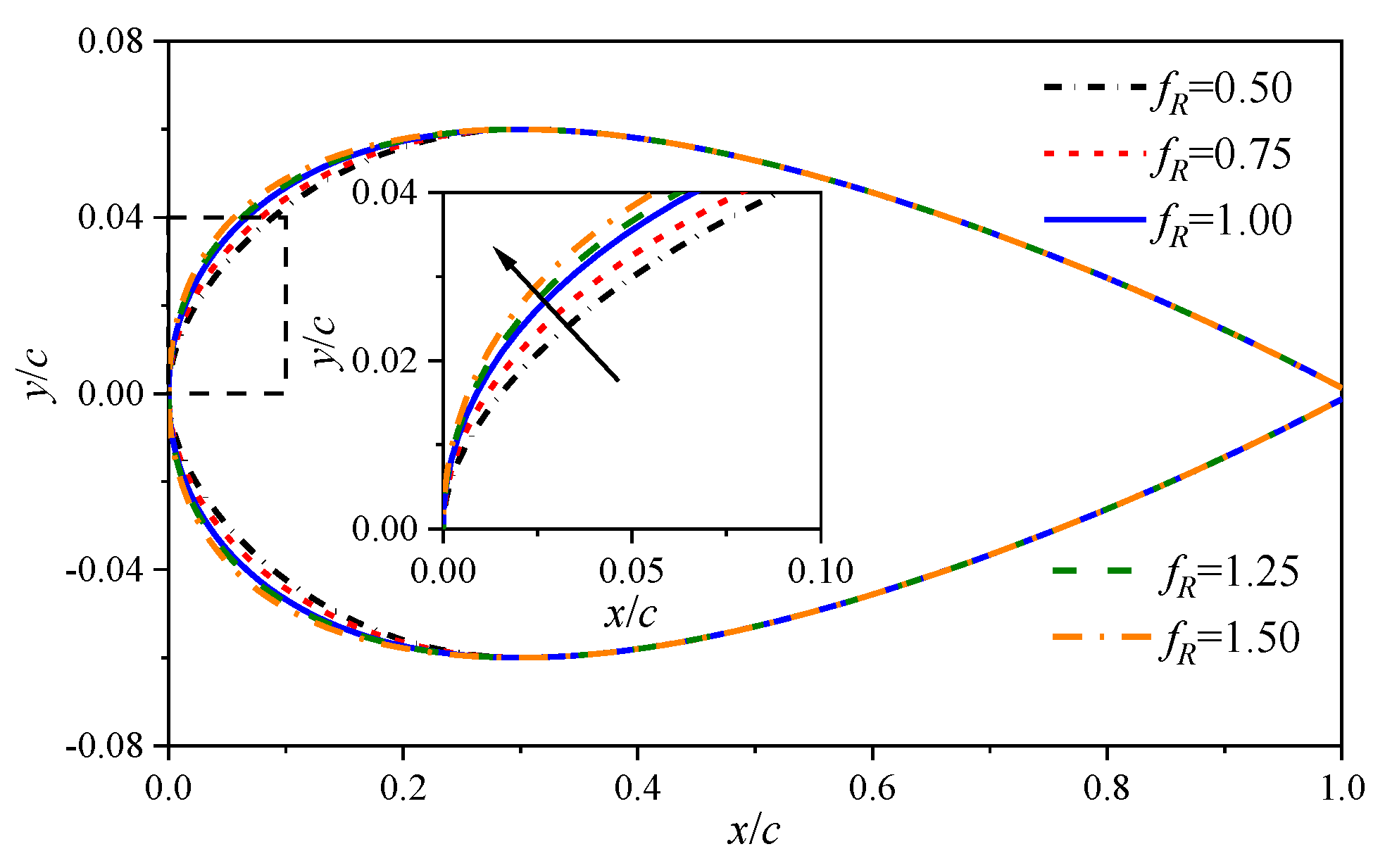
2.1. Airfoil Parametrization Method

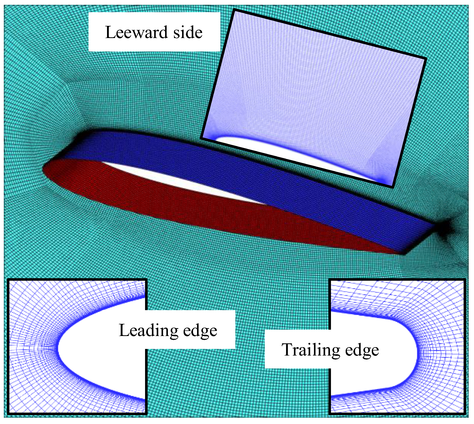
PARFOIL is an airfoil parametrization method developed by Lim [29]. This method performs parametrization based on a baseline airfoil and considers several parameters including leading edge radius. In order to investigate the effect of leading edge radius on aerodynamic stall characteristics of the airfoil, four morphed airfoil geometries are obtained using the PARFOIL method with a NACA 0012 airfoil chosen as the baseline. The updated leading edge radius R_le is obtained by multiplying a scaling factor f_R and the baseline leading edge radius R_le,bl.

$$R_{le}=f_R\cdot R_{le,bl}=\frac{1}{2}{a}_0^2$$

(1)

Then the updated airfoil ordinate of the upper surface y_u(x) in the leading edge region is calculated as follows:

$$y_u\left(x\right)=a_0\sqrt{x}+a_{1}x+a_2{x}^2$$

(2)

where

$$a_1=\frac{2t_0}{x_0}-\frac{3}{2}\frac{a_0}{\sqrt{x_0}}$$

(3)

$$a_2=-\frac{t_0}{x_0^2}+\frac{a_0}{2x_0^{3/2}}$$

(4)

In the above expressions, a₀ is calculated in Equation (1), and t₀ is the corresponding thickness at the thickness crest position x₀. When x = x₀, y_u = t₀. The updated airfoil coordinate of the lower surface is calculated using Equation (2) with an opposite sign.

The leading edge radius of the baseline NACA 0012 airfoil R_le,bl = 0.0159c. The leading edge radius of the four morphed airfoils is 0.5 R_le,bl, 0.75 R_le,bl, 1.25 R_le,bl, 1.5 R_le,bl, with a scaling factor of f_R = 0.5, 0.75, 1.25, 1.5, respectively. f_R = 1.0 denotes the baseline airfoil. The comparisons of NACA 0012 and the four morphed airfoils are shown in Figure 1.

2.2. CFD Method

The Reynolds-averaged Navier–Stokes (RANS) equations serve as the governing equations and are solved using the in-house code CLORNS [30] to determine the flowfield around the airfoil. These equations can be expressed as follows:

$$\frac{\partial }{\partial t}{\displaystyle {\int }_{\Omega }Wd\mathrm{\Omega }}+{\displaystyle {\oint }_{\partial \mathrm{\Omega }}\left({\mathit{F}}_c-{\mathit{F}}_v\right)·\mathit{n}dS}=0$$

(5)

where, ∂Ω denotes the boundary of a control volume Ω; n is the unit normal vector of the surface element dS; W, F_c and F_v are the vector of conserved variables, convective fluxes, and viscous fluxes, respectively.

The k-ω shear stress transport (SST) turbulence model is adopted to account for the effects of turbulence. The governing equations of the SST model read as:

$$\frac{\partial \left(\rho k\right)}{\partial t}+\nabla \cdot \left(\rho \mathit{V}k\right)=P_k-\rho \sqrt{k^3}/l_{RANS}+\nabla \cdot \left[\left({\mu }_l+{\sigma }_k{\mu }_t\right)\nabla k\right]$$

(6)

$$\frac{\partial \left(\rho \omega \right)}{\partial t}+\nabla \cdot \left(\rho \mathit{V}\omega \right)=\frac{\alpha \rho }{{\mu }_t}{P}_k-\beta \rho {\omega }^2+\nabla \cdot \left[\left({\mu }_l+{\sigma }_{\omega }{\mu }_t\right)\nabla \omega \right]+2\left(1-F_1\right)\rho {\sigma }_{\omega 2}\frac{\nabla k\cdot \nabla \omega }{\omega }$$

(7)

where, k and ω are the turbulent kinetic energy and its specific dissipation rate, respectively. F₁ is the blending function. The terms on the right-hand side of Equations (6) and (7) represent eddy-viscosity production, dissipation, and conservative diffusion, respectively. The production term reads as follows:

$$P_k=\min \left({\mu }_t{S}^2,10C_{\mu }\rho k\omega \right)$$

(8)

The RANS length scale in Equation (6) reads as follows:

$$l_{RANS}=k^{1/2}/\left(C_{\mu }\omega \right)$$

(9)

A hybrid RANS-LES method is conducted using the improved delayed detached-eddy simulation (IDDES) model based on the SST turbulence model [31]. The RANS length scale in Equation (6) is replaced by the IDDES length scale in the SST IDDES formulations. The IDDES length scale reads as follows:

$$l_{IDDES}={\tilde{f}}_d\cdot l_{RANS}+\left(1-{\tilde{f}}_d\right)\cdot l_{LES}$$

(10)

Here ${\tilde{f}}_d$ denotes the empiric blending function, $l_{LES}$ denotes the LES length scale. For detailed formulas, please refer to Reference [31].

2.3. Validation for CFD Method

To enhance confidence in the above methodology, a series of simulations are conducted, including the airloads of both static and pitching airfoils, as well as the grid and time step convergence.

2.3.1. Static NACA 0012 Airfoil

The RANS method is employed to simulate the aerodynamic characteristics of static airfoils. Three O-type grids are generated to compute the aerodynamic behaviors of a static NACA 0012 airfoil for the purpose of grid independence study. The grid information is detailed in

Table 1. Detailed information of grids for static NACA 0012 airfoil.

Grid Resolution	Number of Grid Points
Coarse	248 × 95
Medium	306 × 112
Fine	421 × 142

. The outer boundary is located 20c away from the airfoil. The height of the first mesh cell off the airfoil wall is 4 × 10⁻⁶c to ensure the y⁺ < 1.

Figure 2 compares the numerical and experimental airloads [15] of NACA 0012 airfoil at a Mach number of 0.3 and a Reynolds number of 3.7 × 10⁶. The RANS method underestimates the lift and nose-down pitching moment at high angles. Nevertheless, the predicted stall angle and pre-stall lift agree well with the experimental results. Also, the computed drag and pitching moment before the stall matches the experimental data closely. Overall, the three grids yield comparable results, suggesting satisfactory grid convergence. The subsequent simulations of static airfoils employ the fine grid.

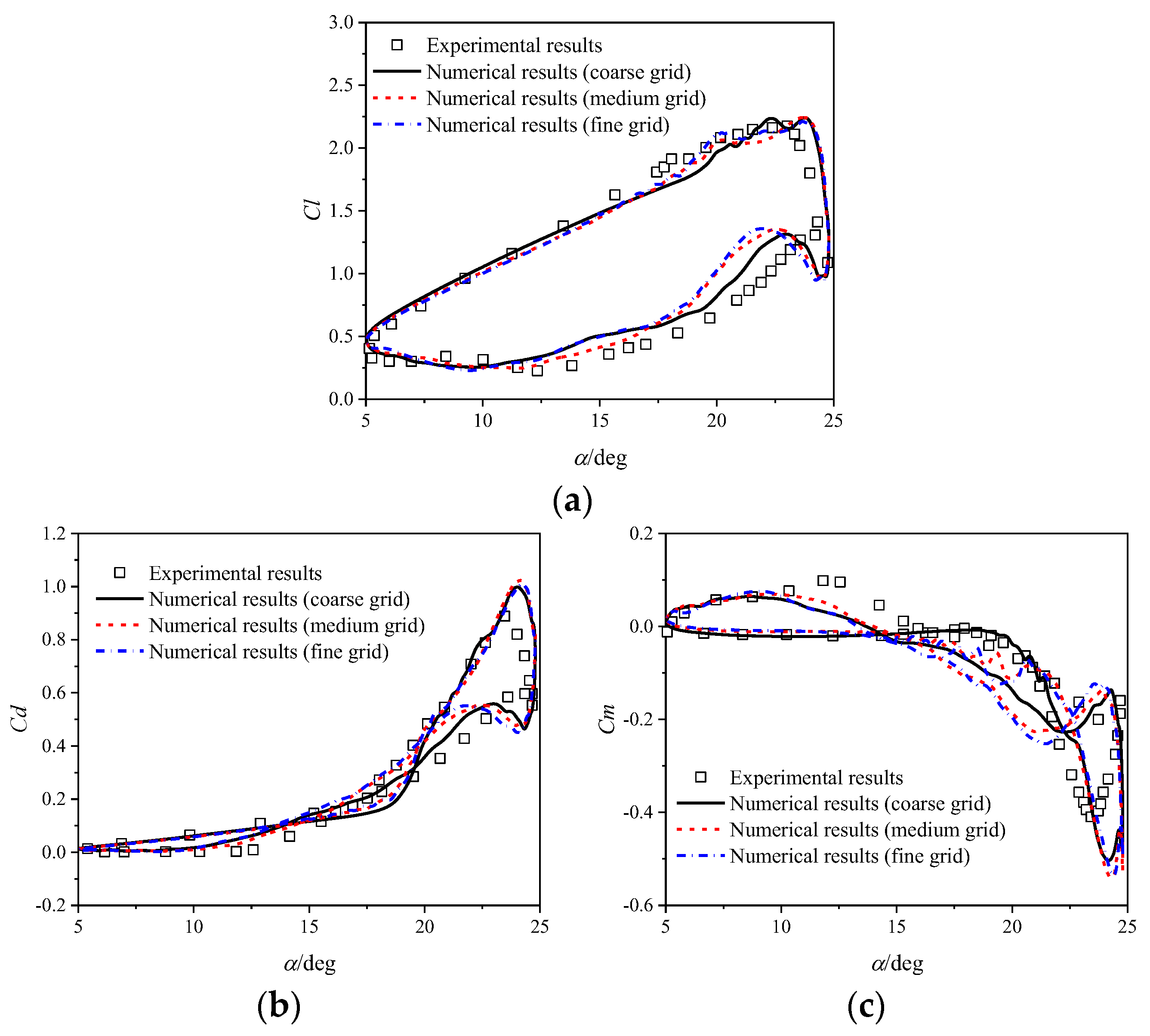
2.3.2. Pitching NACA 0012 Airfoil

The IDDES method is employed for pitching airfoils. In contrast to RANS, IDDES cannot reach a grid and time step-independent solution as typically achieved by RANS solvers [32,33]. Nevertheless, the IDDES simulations of a pitching NACA 0012 airfoil are conducted using different grids and time steps.

The aerodynamic behaviors of the pitching NACA 0012 airfoil are simulated using three sliding grids with information detailed in

Table 2. Detailed information of grids for pitching NACA 0012 airfoil.

Grid Resolution	Total Number of Grid Points	Cell Size in the LES Region
Coarse	248 × 95 × 51	0.02c
Medium	306 × 112 × 67	0.015c
Fine	421 × 142 × 101	0.01c

. The computational domain has a radius of 20, featuring a sliding interface with a radius of 5c. The grids in the LES region are approximately homogeneous and isotropic. Figure 3 illustrates the grid arrangement around the NACA 0012 airfoil. Both spanwise ends use a periodic boundary condition.

The NACA 0012 airfoil is subjected to a pitching motion with an angle of α = 14.91° + 9.87° sin(ωt), a reduced frequency of k = 0.151, a Mach number of Ma = 0.283, and a Reynolds number of Re = 3.45 × 10⁶. Figure 4 compares the numerical results obtained from three time steps based on the medium grid. Figure 5 compares the numerical results obtained from three grids and experimental data [16]. The IDDES method overpredicts the stall angle and peak values of drag and nose-down pitching moment. The numerical results bear a high degree of similarity during the pitching-up stage. Some discrepancies are observed during the recovery stage, which is acceptable for the purpose of this research. Overall, the numerical results exhibit a favorable agreement with the experimental results. The results of these validations demonstrate the effectiveness of CFD methods for the analysis of stall behaviors in both static and pitching airfoils.

3. Results and Discussions

3.1. Impacts on Static Aerodynamic Characteristics

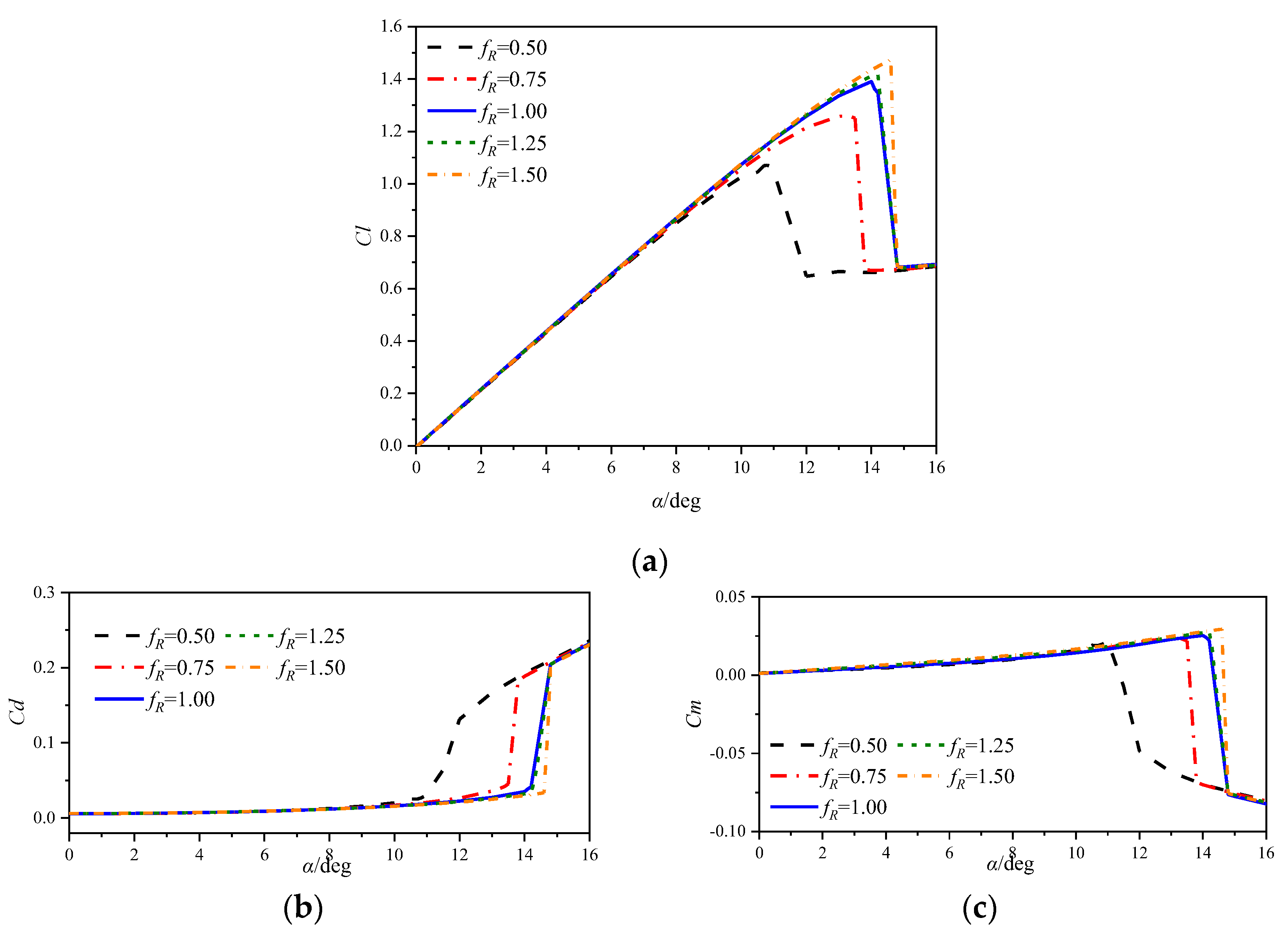
3.1.1. Static Cases at a Mach Number of 0.283

The simulations of the static airfoils are conducted at a Mach number of 0.283 with a Reynolds number of 3.5 × 10⁶. Figure 6 displays the aerodynamic force coefficients of the airfoils. The leading edge radius has little influence on the lift slope but significantly affects the static stall characteristics. Increasing the leading edge radius delays the lift stall, drag divergence and pitching moment divergence. Moreover, the maximum lift coefficient shows an increasing trend with increasing leading edge radius, but at a very small rate when f_R > 1. When AoA exceeds the stall angle, the airfoil encounters a sharp decline in lift coefficient, while a rapid rise in drag and nose-down moment coefficients, indicating an abrupt stall.

Figure 7, Figure 8 and Figure 9 illustrate the skin friction and pressure coefficient distributions of airfoils near stall. The static stall angles for the airfoil with f_R = 0.50, 1.00, and 1.50 are approximately 10.8°, 14.0°, and 14.6°, respectively. The negative value of skin friction indicates the occurrence of flow separation.

For the airfoil with f_R = 0.50, localized leading edge separation is observed at α = 9°, as shown in Figure 7a. As AoA increases, the separation point moves upstream and the suction pressure peak increases, as shown in Figure 7b. When the airfoil exceeds the stall angle, a sudden and complete flow separation occurs, causing an abrupt drop in the suction pressure peak. As a result, stall events such as the lift stall, drag divergence, and pitching moment divergence arise.

The other two airfoils with f_R = 1.00 and 1.50, shown in Figure 8 and Figure 9, exhibit a stall process similar to that of the airfoil with f_R = 0.50. This suggests that all the airfoils experience leading edge stall at the Mach number of 0.283. The increase in the leading edge radius does not alter the type of leading edge stall but results in the postponement of leading edge flow separation and stall onset.

It is observed that an increased leading edge radius causes the airfoil to experience a more significant decrease in the suction pressure peak. This is evident from the blue arrows in the Cp figures. Consequently, the airfoil with a greater leading edge radius exhibits a higher magnitude of variation in airloads after stall, aligning with the results presented in Figure 6.

Figure 10, Figure 11 and Figure 12 display the pressure coefficient contours and streamlines surrounding the airfoils with f_R = 0.50, 1.00, and 1.50. A localized trailing edge separation (TES) occurs on the airfoils before stall onset. As the AoA of the airfoil exceeds the stall angle, all airfoils experience complete flow separation. However, the size of separation vortices varies. The airfoil with a greater leading edge radius generates a larger separation vortex after stall onset (indicated by the blue arrows), resulting in a greater reduction in suction pressure peak. Generally, an increase in leading edge radius delays the stall onset. Once stall occurs, the airfoil with a greater leading edge radius encounters a greater loss in aerodynamic performance.

Figure 13 illustrates the relationship between the minimum pressure coefficient and the AoA. An increase in leading edge radius results in a slower increase in the amplitude of the suction pressure peak with respect to AoA.

Figure 14 displays the pressure coefficient distribution of airfoils at α = 2° and 8°. Airfoils with larger leading edge radii generate higher suction pressure peaks and adverse pressure gradients at lower AoAs. Conversely, at higher AoAs, these airfoils generate smaller suction pressure peaks and adverse pressure gradients. Flow separation mainly occurs at high AoAs due to the presence of significant adverse pressure gradients. At high AoAs, a larger leading edge radius mitigates the suction pressure peak and adverse pressure gradient, thus delaying flow separation and the onset of leading edge stall.

3.1.2. Static Cases at a Mach Number of 0.5

The aerodynamic characteristics at a Mach number of 0.5 and a Reynolds number of 3.5 × 10⁶ are simulated for the airfoils with various leading edge radii. Figure 15 shows the aerodynamic force coefficients of the airfoils. The pre-stall airloads of the airfoils exhibit a high degree of similarity, particularly in the linear-lift stage. At the high Mach number of 0.5, the airfoils encounter stall at lower AoA (≈9.2°) and show a moderate change in aerodynamic force coefficient after stall, compared to the cases at the low Mach number of 0.283. Moreover, the variations in the leading edge radius indicate a minimal effect on static stall behaviors, such as the stall angle and airloads near stall.

Figure 16a displays the pressure coefficients of the NACA 0012 airfoil at various AoAs. The critical pressure coefficient Cp_cr obtained from the isentropic relation is also shown in the figure. As the AoA exceeds 5°, the pressure coefficient near the leading edge starts to exceed the critical value, indicating the occurrence of local supersonic flow. When the AoA reaches 7°, a shock wave is observed at the leading edge. With increasing AoA, the extent of supercritical flow increases and the shock wave moves downstream and strengthens. However, when the AoA reaches 10°, the shock wave starts to move upstream. The pressure behind the shock wave also decreases.

Figure 16b shows the skin frictions over the suction side of the NACA 0012 airfoil. The red color in the Cf distribution highlights the occurrence of negative skin friction, which refers to the region of flow separation. At low AoAs (α ≤ 6°), the airflow fully attaches to the airfoil surface. As the AoA reaches 7°, the airfoil experiences localized flow separation near the leading edge. The separation region expands with increasing AoA. Figure 17 shows the contours of the pressure coefficient of the NACA 0012 airfoil at α = 7° and 8°. A shock wave forms near the leading edge and causes the localized flow separation, as indicated by the velocity profiles. This reveals that the deceleration of lift increase before stall is caused by the expansion of shock-induced separation.

At α = 9°, two separation points are observed on the airfoil: the shock-induced leading edge separation and the trailing edge separation, as depicted in Figure 16b. After the onset of stall, the two separated regions expand and eventually merge, creating a reverse flow across the entire upper surface. As the AoA increases, this reverse flow gradually enlarges (shown in Figure 18), leading to a smooth post-stall behavior in the airloads, as shown in Figure 15.

Figure 19 illustrates the pressure coefficients and skin frictions for the airfoil with f_R = 1.50. The critical pressure coefficient Cp_cr is also shown in Figure 19a. The stall process of the airfoil is similar to that of the NACA 0012 airfoil. Additionally, the other three airfoils with f_R = 0.50, 0.75, and 1.25 undergo the same stall process. The results suggest that modifying the leading edge radius does not change the shock-induced stall regime.

Figure 20 compares distributions of the pressure coefficient for the airfoils with various leading edge radii before stall. With increasing leading edge radius, the shock wave moves aft on the chord and decreases in intensity, indicating reduced compressibility effects. However, the increased leading edge radius has minimal impacts on the high adverse pressure gradient near the shock wave. Hence, the airfoils with distinct leading edge radii show similar static stall characteristics.

3.2. Impacts on Dynamic Stall Characteristics

The dynamic stall characteristics of airfoils with various leading edge radii are simulated at Mach numbers of 0.283 and 0.5. The simulations subject the airfoil to pitching oscillations, with the AoA defined by the equation α = 14.91° + 9.87° sin(ωt), where ω = 48.63 rad/s. The reduced frequencies at Ma = 0.283 and 0.5 are determined to be 0.151 and 0.085, respectively.

3.2.1. Dynamic Cases at a Mach Number of 0.283

Figure 21 presents the aerodynamic force coefficients at a Mach number of 0.283 for airfoils. All five airfoils exhibit similar dynamic stall characteristics. The main differences arise in the stall development and post-stall stages.

Figure 22 illustrates the effect of leading edge radius on the stall angle and peak value of the force coefficient. An increasing trend is observed in the static stall angle, dynamic moment stall angle, and dynamic lift stall angle as the leading edge radius increases. Moreover, the peak value of the force coefficient exhibits an increasing trend with the increasing leading edge radius. However, the effects of leading edge radius on the peak value of force coefficient in dynamic cases is much smaller compared to that in static cases.

Figure 23 displays the contours of the spanwise averaged pressure coefficient for airfoils during the pitching-up process. In the pitching-up circle, airfoils experience an increase in the suction peak, reaching a similar maximum value. However, the airfoil with a larger leading edge radius takes longer to achieve this maximum value. Three events are observed in the pitching-up circle, such as trailing edge separation, a sudden loss of suction peak, and the convection of DSV.

The critical pressure coefficient Cp_cr for the sonic flow obtained from the isentropic relation is also shown in Figure 23. The pressure coefficient near the leading edge starts to exceed the critical value at α ≈ 12°, 14°, and 15° for the airfoil with f_R = 0.50, 1.00, and 1.50, respectively. This indicates that supersonic flow appears near the leading edge. The supersonic region persists until the sudden collapse of suction pressure. Unsteady motion delays the stall to a higher AoA compared to the static cases. As a result, compressibility effects are observed for the dynamic cases at the Mach number of 0.283.

Figure 24 illustrates the distributions of spanwise averaged skin friction of airfoils (f_R = 0.5, 1.0, and 1.5) before the collapse of the suction pressure peak. Negative Cf is colored by red indicating the presence of flow separation. An increase in the leading edge radius delays the leading edge separation to a higher AoA. As the airfoil pitches up, the leading edge separation region gradually expands. The DSV forms near the leading edge shortly after the collapse of the suction peak, indicating that the airfoil encounters a leading edge stall.

Figure 25a shows the spanwise averaged pressure coefficient near the collapse of the suction pressure peak in the vicinity of the leading edge. No visible shock wave is observed, despite the existing local supersonic flow near the leading edge. The high adverse pressure gradient near the leading edge is the main cause of flow separation.

Figure 25b compares the pressure coefficient distribution of the airfoils at α = 15.22° in the pitching-up circle. An increase in leading edge radius reduces the suction pressure peak and adverse pressure gradient, hence delaying the leading edge separation and dynamic stall.

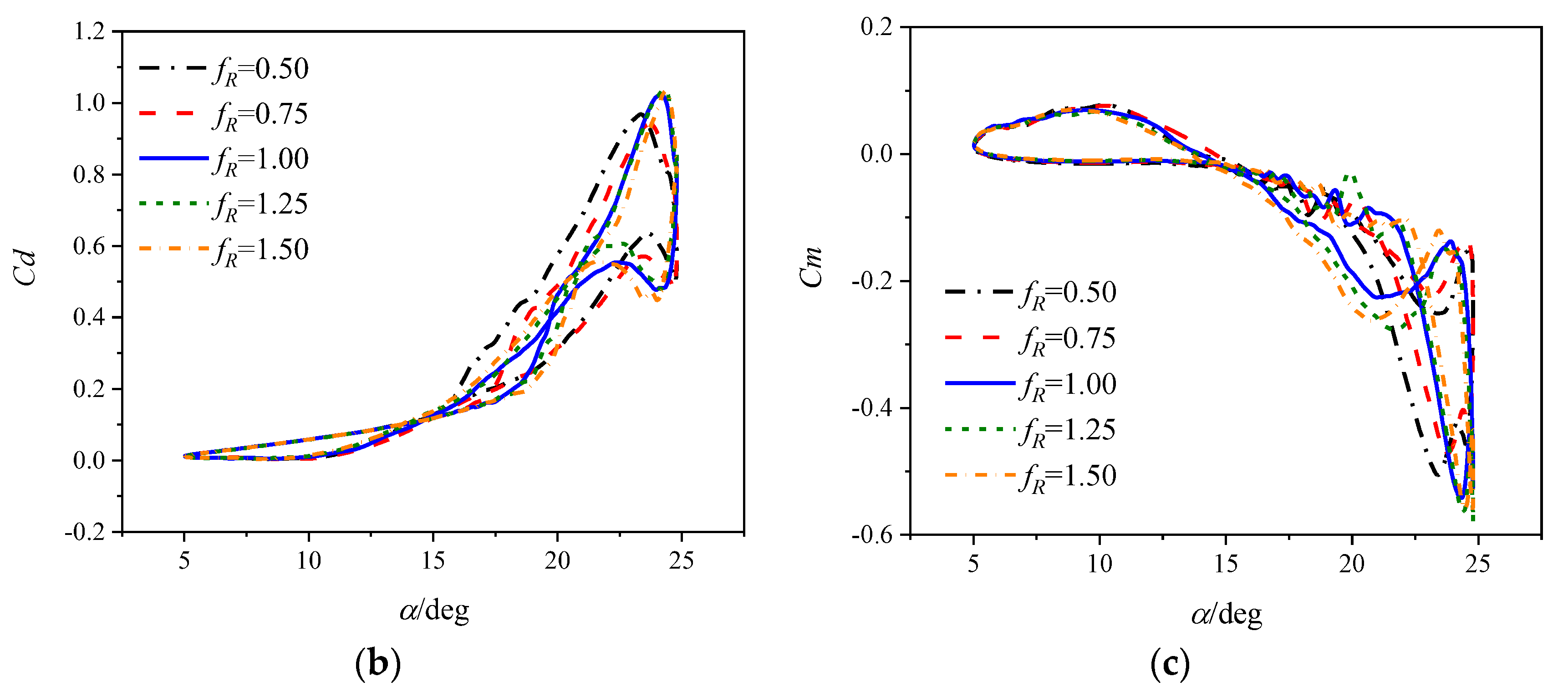
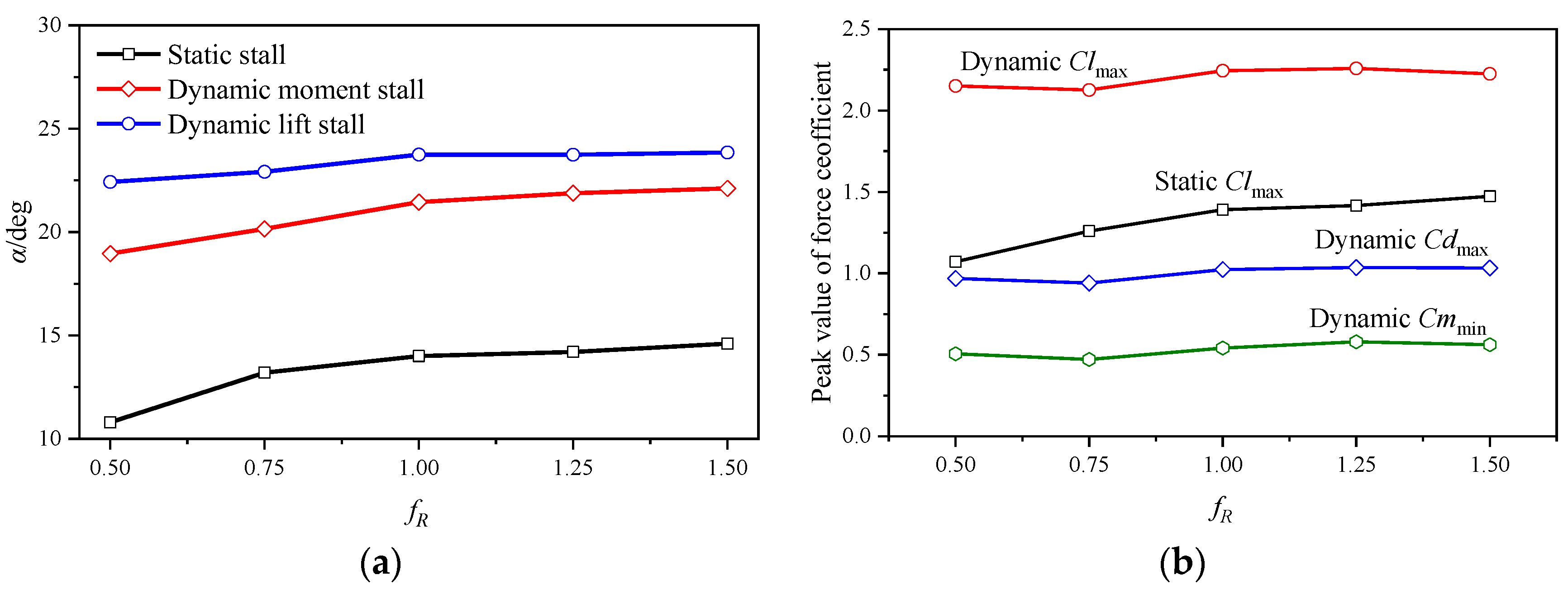
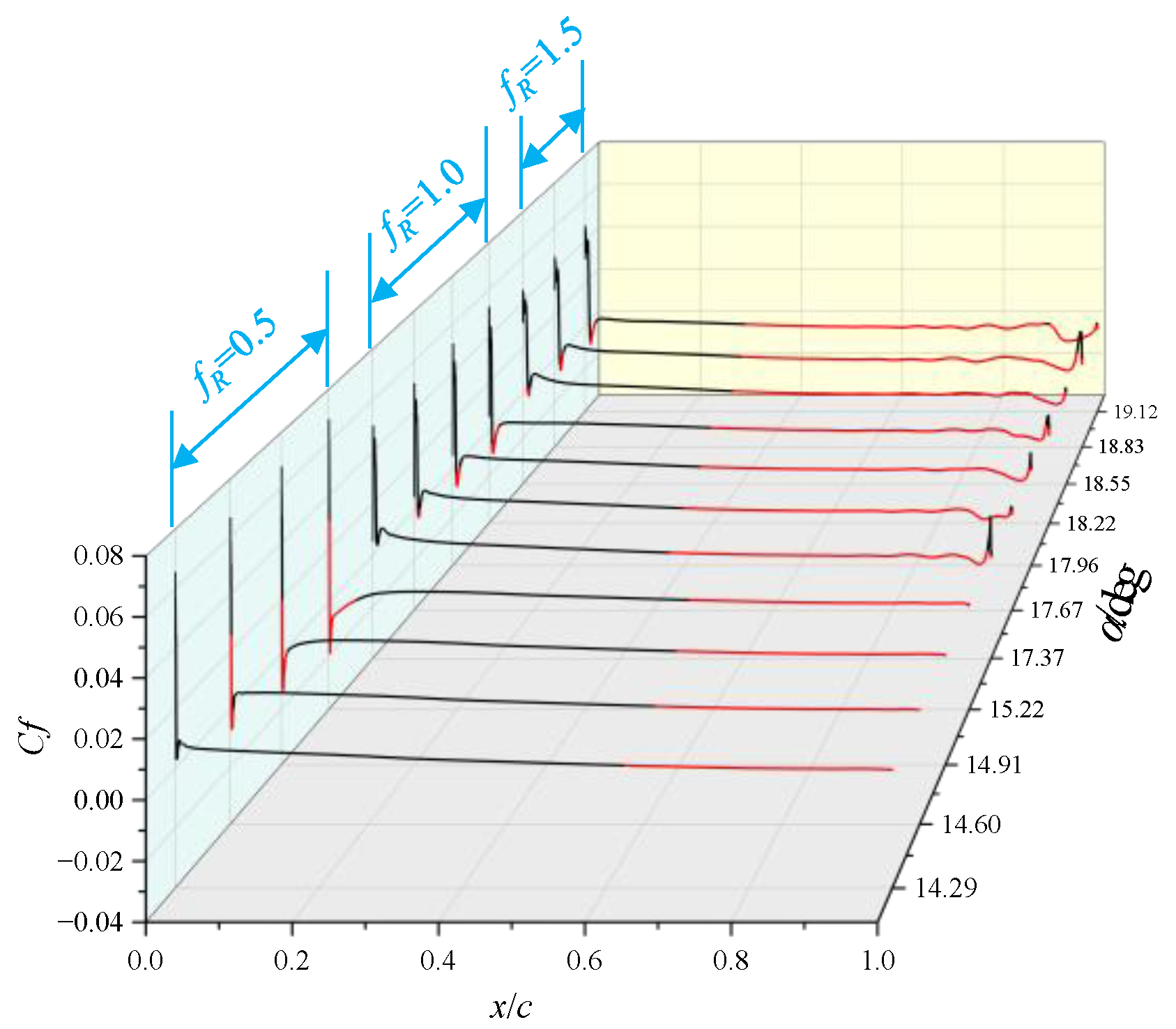
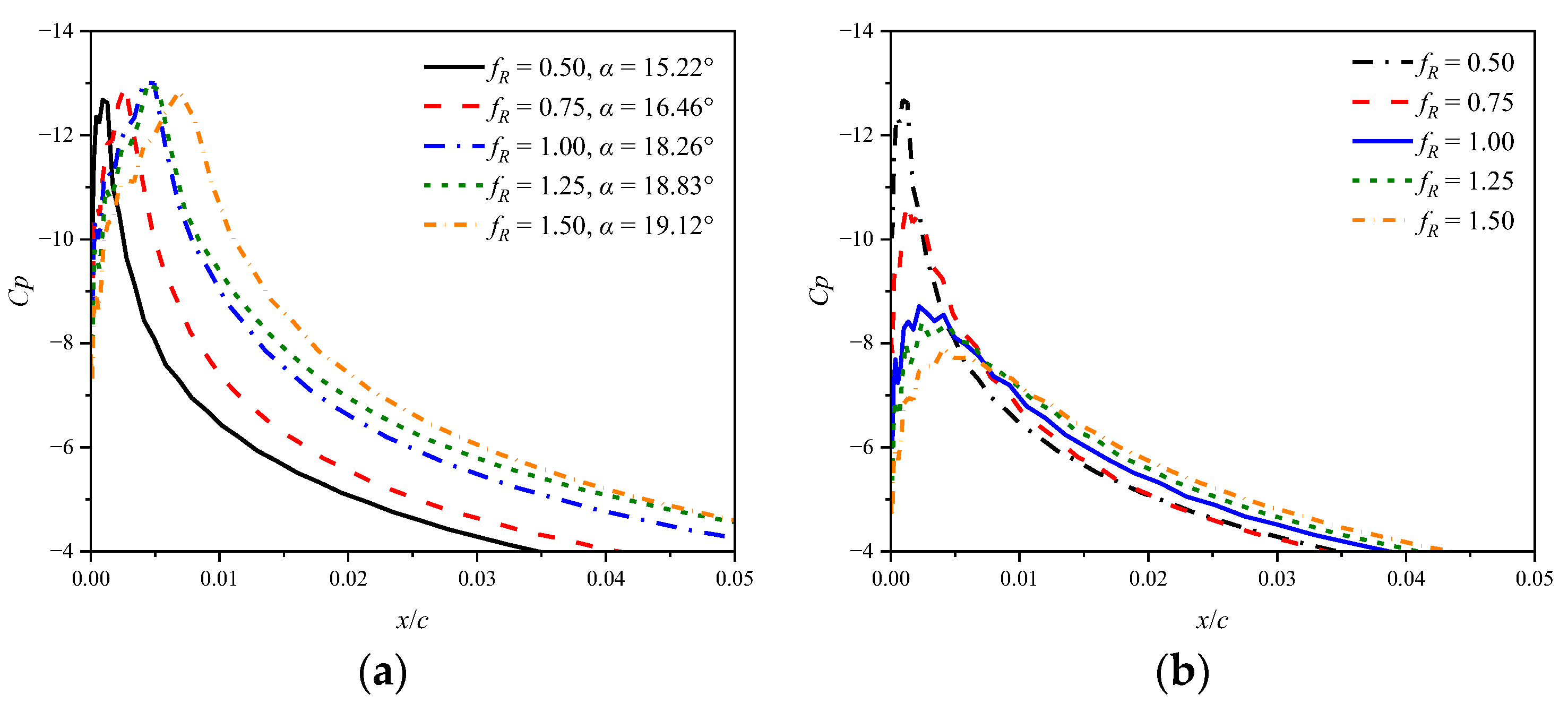
3.2.2. Dynamic Cases at a Mach Number of 0.5

Figure 26 shows the aerodynamic force coefficients of the airfoils with f_R = 0.5, 1.0, and 1.5 at a high Mach number of 0.5. Compared to the Mach number of 0.283, airfoils encounter moment stall, drag divergence and lift stall at lower AoAs at the high Mach number of 0.5. Moreover, the aerodynamic force coefficient shows a gradual change after the occurrence of stall. The three airfoils with different radii exhibit similar aerodynamic force hysteresis and dynamic stall angles. Compared to the cases at low Mach numbers, the impact of leading edge radius on dynamic aerodynamic characteristics is minimal at high Mach numbers.

Figure 27 displays the contours of the spanwise averaged pressure coefficient of airfoils in the pitching-up circle. The critical pressure coefficient Cp_cr is also given in the figures. At the Mach number of 0.5, the flow at the leading edge of airfoils becomes locally supersonic at a very small AoA due to the significant compressibility effects. The supersonic region persists even after the shedding of DSV. Trailing edge separation, a gradual decrease in suction pressure peak, and the convection of DSV are observed during the pitching-up process. The force coefficient gradually varies after the occurrence of stall due to the gradual decrease in suction pressure peak and the relatively small intensity of the DSV compared to the Mach number of 0.283.

Figure 28 displays the distributions of the spanwise averaged pressure coefficient near the leading edge in the pitching-up circle. At α = 9.10°, a shock wave is observed at the leading edge of airfoils. With increasing leading edge radius, the shock wave moves aft along the chord and weakens, indicating a reduced trend in compressibility effects. As the AoA is increased from 9.10° to 10.42°, the shock wave moves aft and strengthens. Moreover, significant inflection points are observed in the pressure recovery section, as depicted in Figure 28b. This observation signifies the presence of flow separation, which is also evident from the velocity profiles near the shock wave, as shown in Figure 29.

Figure 30a shows the spanwise averaged pressure coefficients of the NACA 0012 airfoil at α = 10.42°, 11.86°, 12.15°, 12.75°, and 13.36° in the pitching-up circle. At α = 10.42°, flow separation induced by a shock wave is observed near the leading edge, as mentioned above. As the AoA is increased from 10.42° to 11.86°, the shock wave starts to move forward, and the pressure behind the shock wave fluctuates and decreases. As the AoA reaches 12.15°, a local negative pressure peak is observed behind the shock wave and moves downstream with further increases in AoA. This indicates the formation and convection of the DSV.

Figure 30b presents the spanwise averaged pressure coefficients over the suction side of the morphed airfoil with f_R = 1.50. The airfoil encounters flow separation induced by a shock wave and shows a similar dynamic stall regime as the baseline NACA 0012 airfoil. The other three airfoils exhibit a comparable behavior.

Figure 31 displays the iso-surface of the Q criterion of the NACA 0012 airfoil at α = 13.36° in the pitching-up circle. At the moment, the center of the DSV is located at a chordwise position of 0.35c, resulting in a dramatic increase in the nose-down pitching moment, as shown in Figure 26c. It can be inferred that the shock-induced flow separation is the primary cause of dynamic stall at the high Mach number of 0.5.

The results indicate that airflow is significantly affected by the compressibility effects at high Mach numbers. The primary cause of dynamic stall is shock-induced flow separation. Increasing the leading edge radius reduces the compressibility effects and weakens the shock wave near the leading edge. Nevertheless, increasing the leading edge radius shows minimal effects on the shock-induced dynamic stall characteristics of airfoils.

4. Conclusions

The effects of the leading edge radius on the static and dynamic stall characteristics of a NACA 0012 airfoil are investigated using the PARFOIL and IDDES methods. The primary conclusions are as follows:

(1)

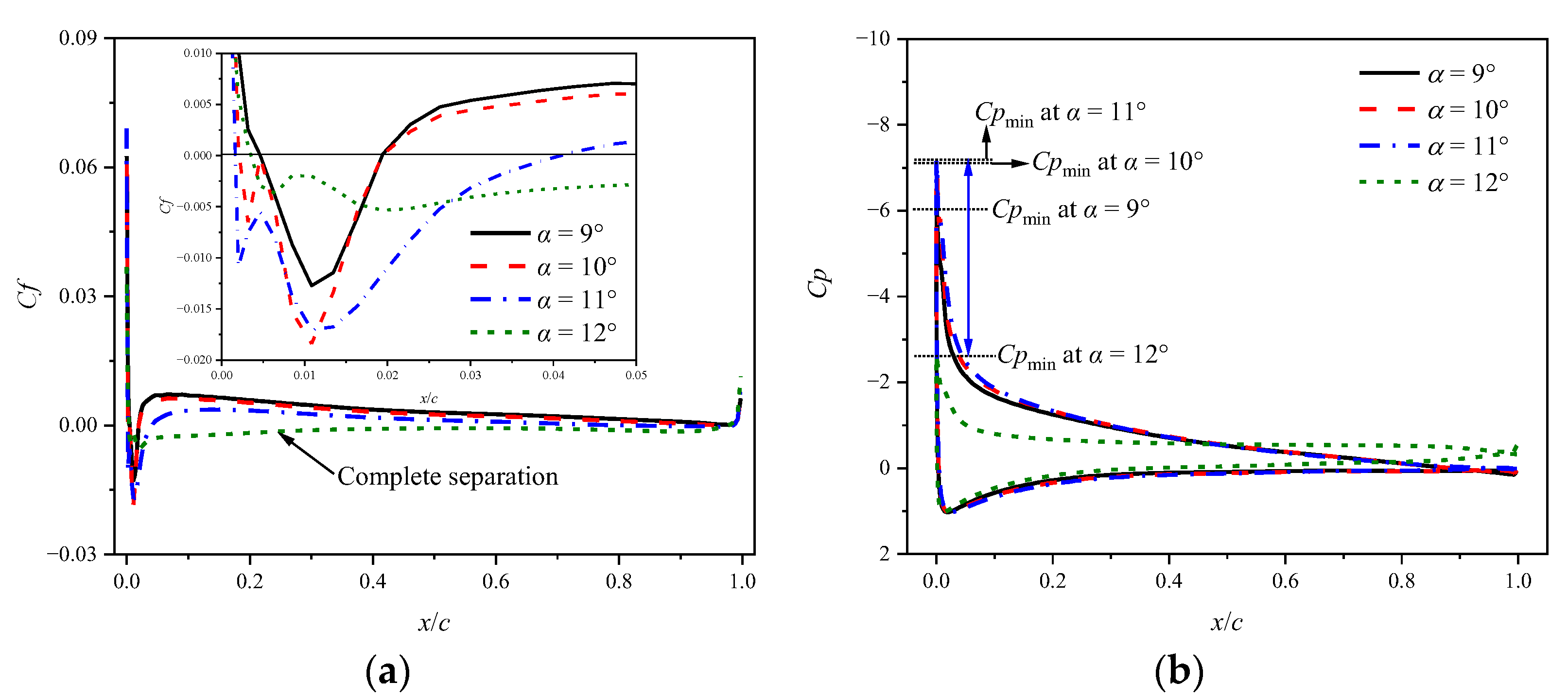
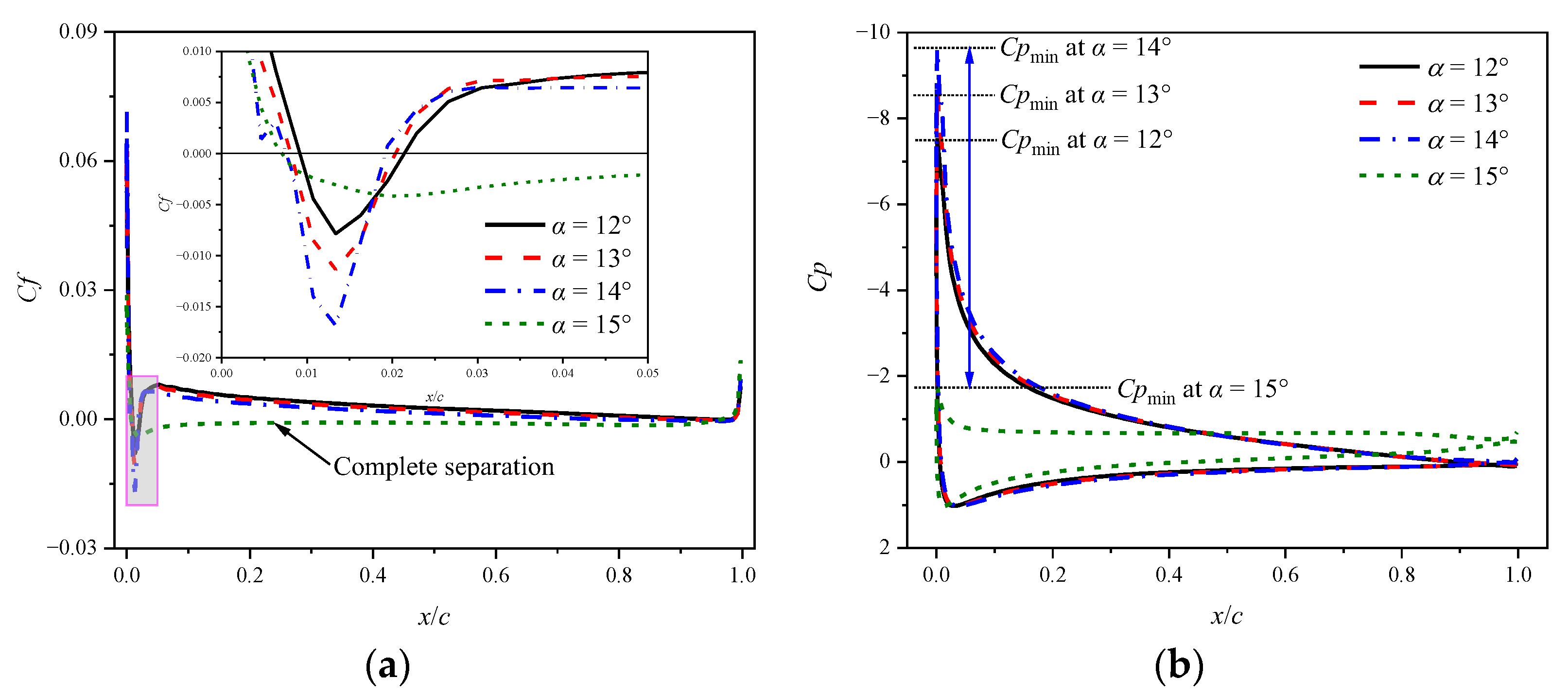
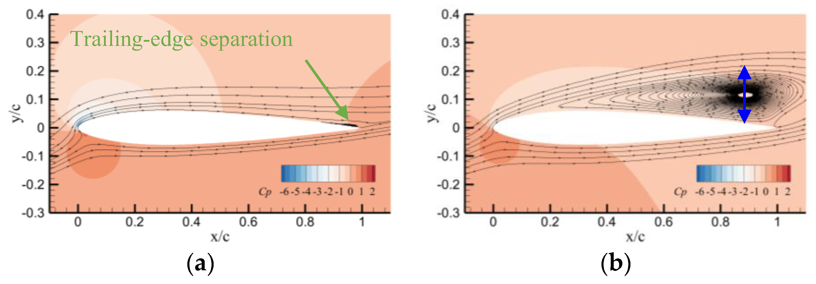
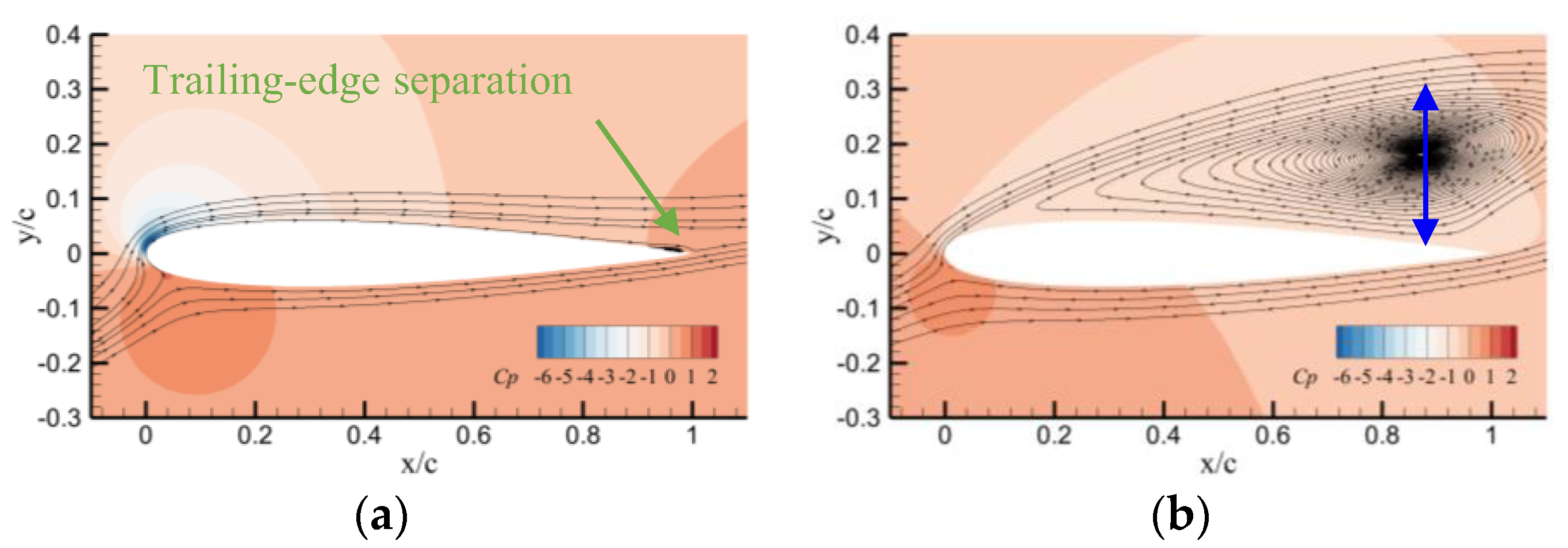
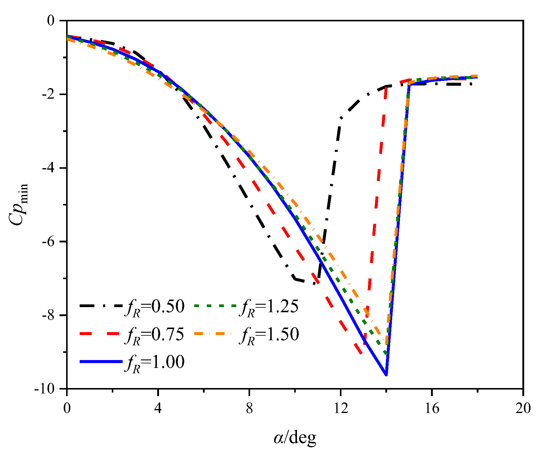
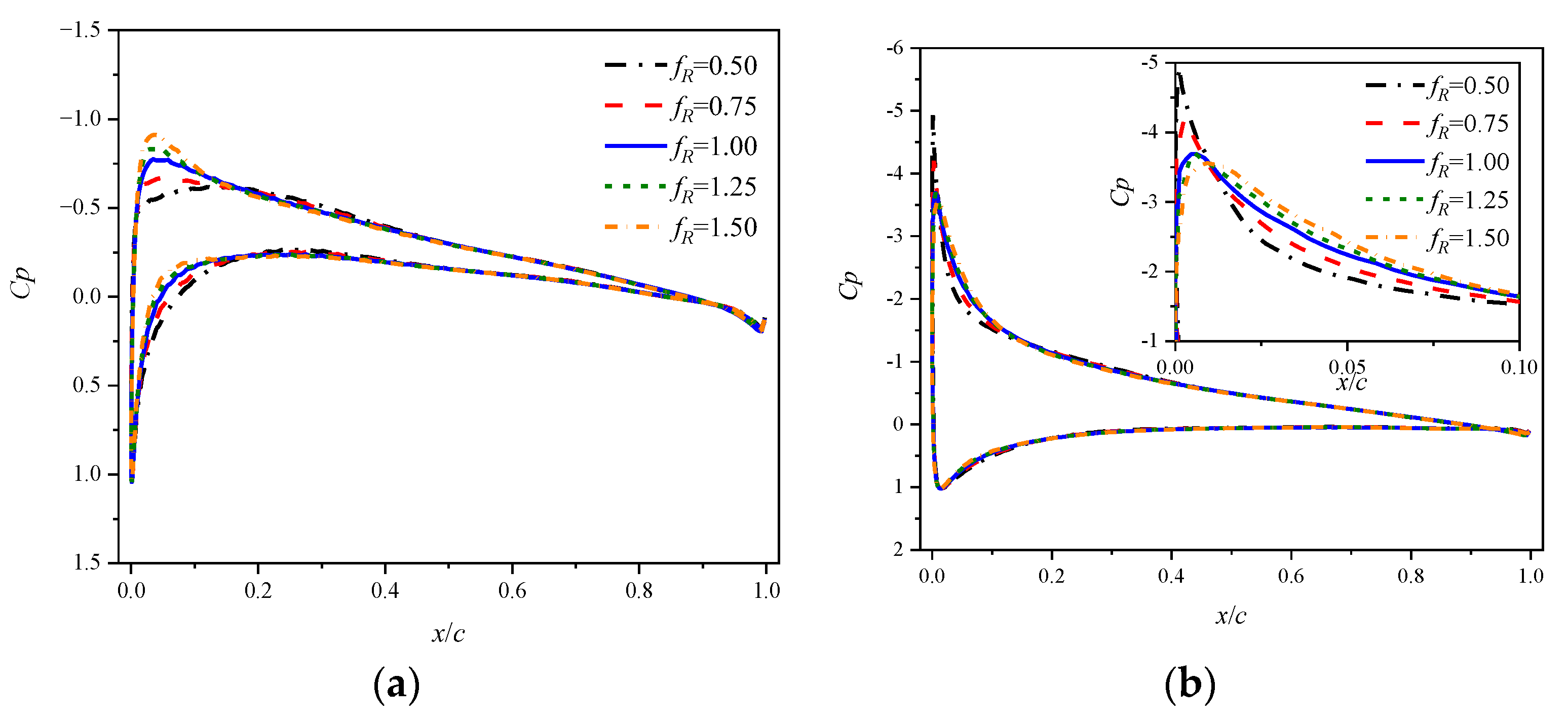
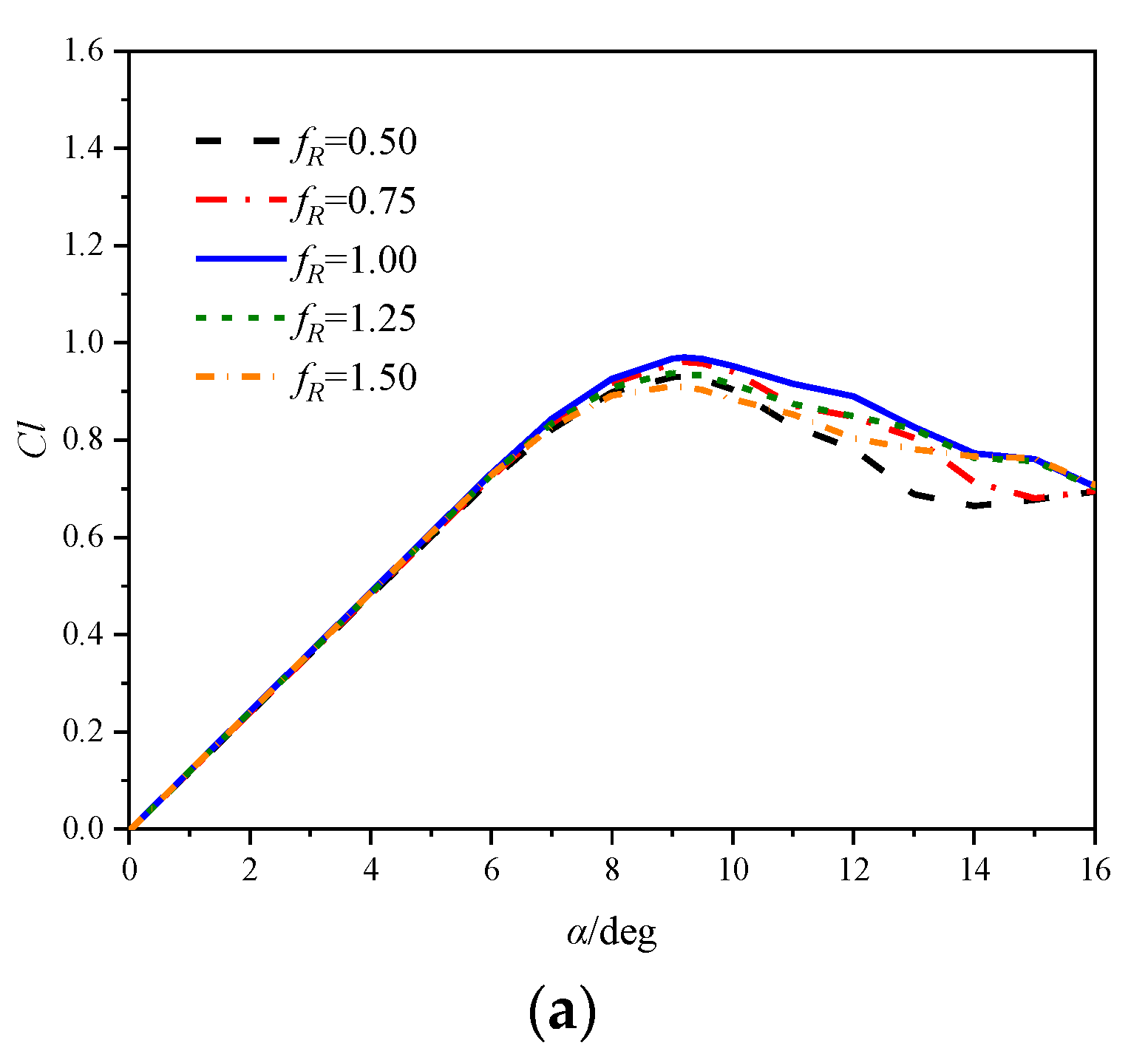
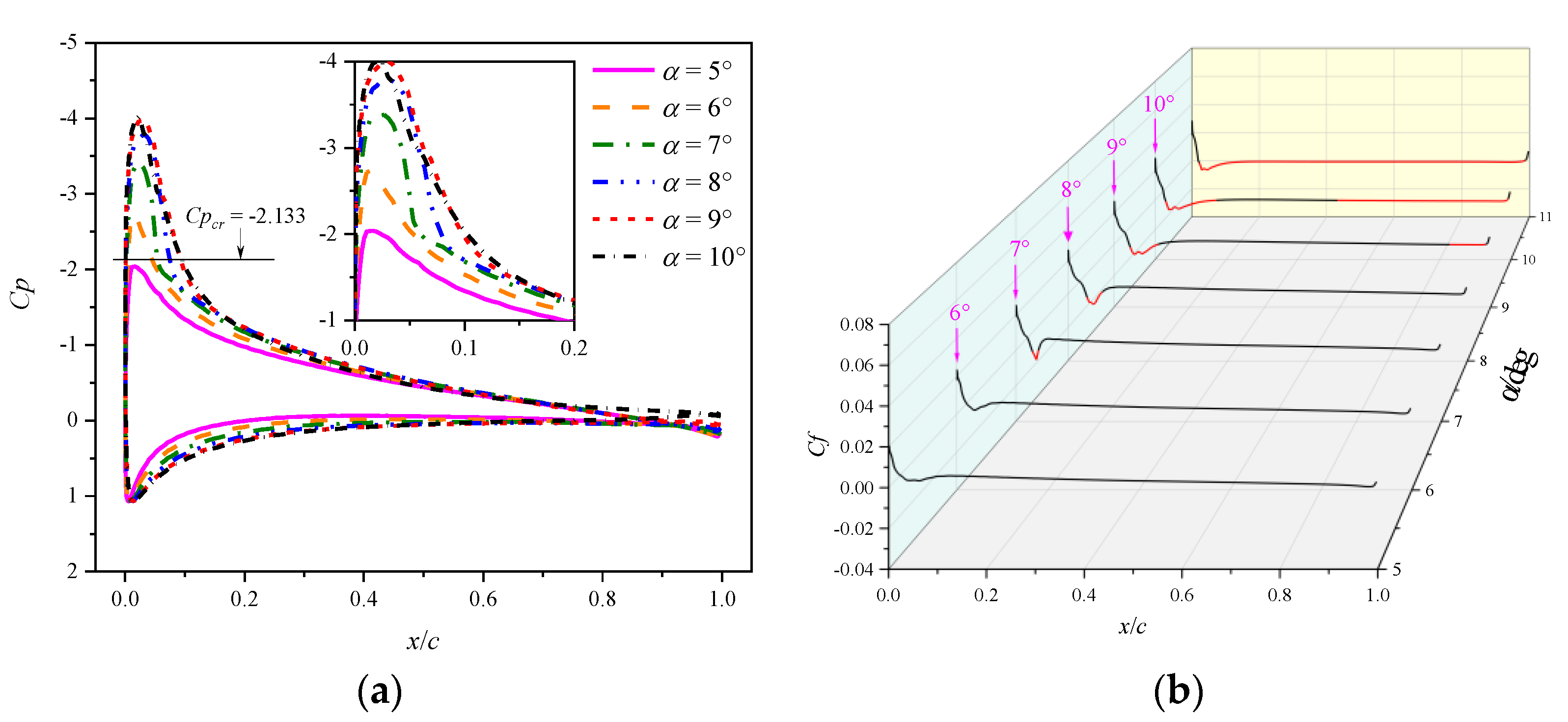
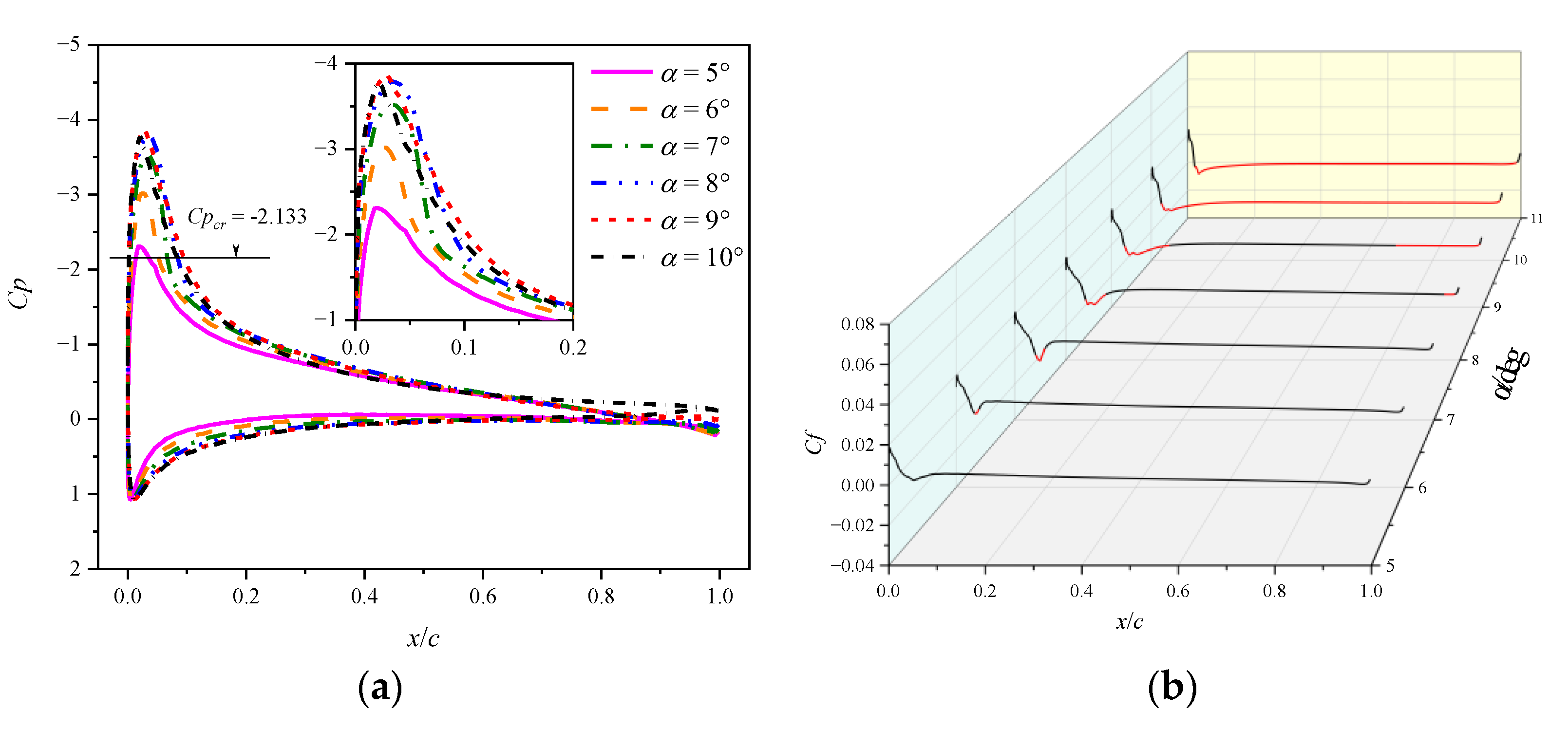
At a low Mach number of 0.283, the airfoil experiences an abrupt leading edge stall in both static and dynamic cases. In the dynamic cases, unsteady motion delays the stall to a higher AoA compared to the static cases, and supercritical flow is observed on the airfoil. Despite the existing local supersonic flow near the leading edge, no visible shock wave is observed. The high adverse pressure gradient near the leading edge is the primary cause of both static and dynamic stall at the low Mach number. The stall regime remains unaffected by variations in the leading edge radius. However, increasing the leading edge radius reduces the suction pressure peak and adverse pressure gradients, hence delaying the leading edge separation and stall.

(2)

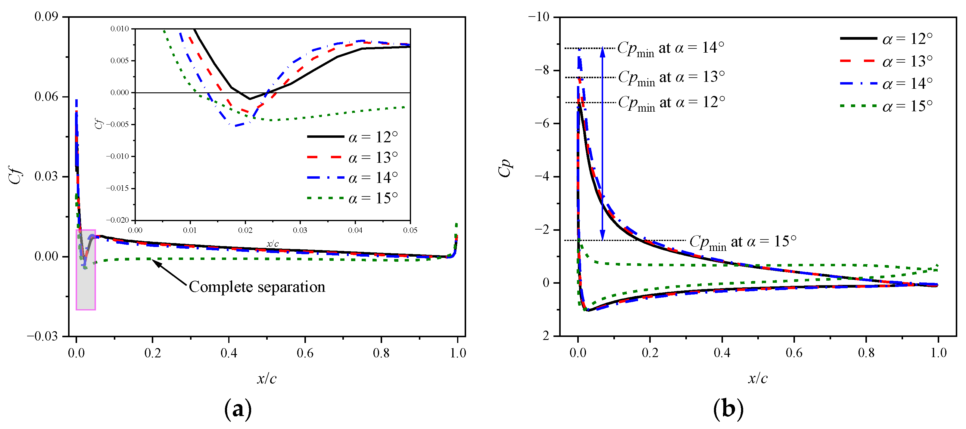
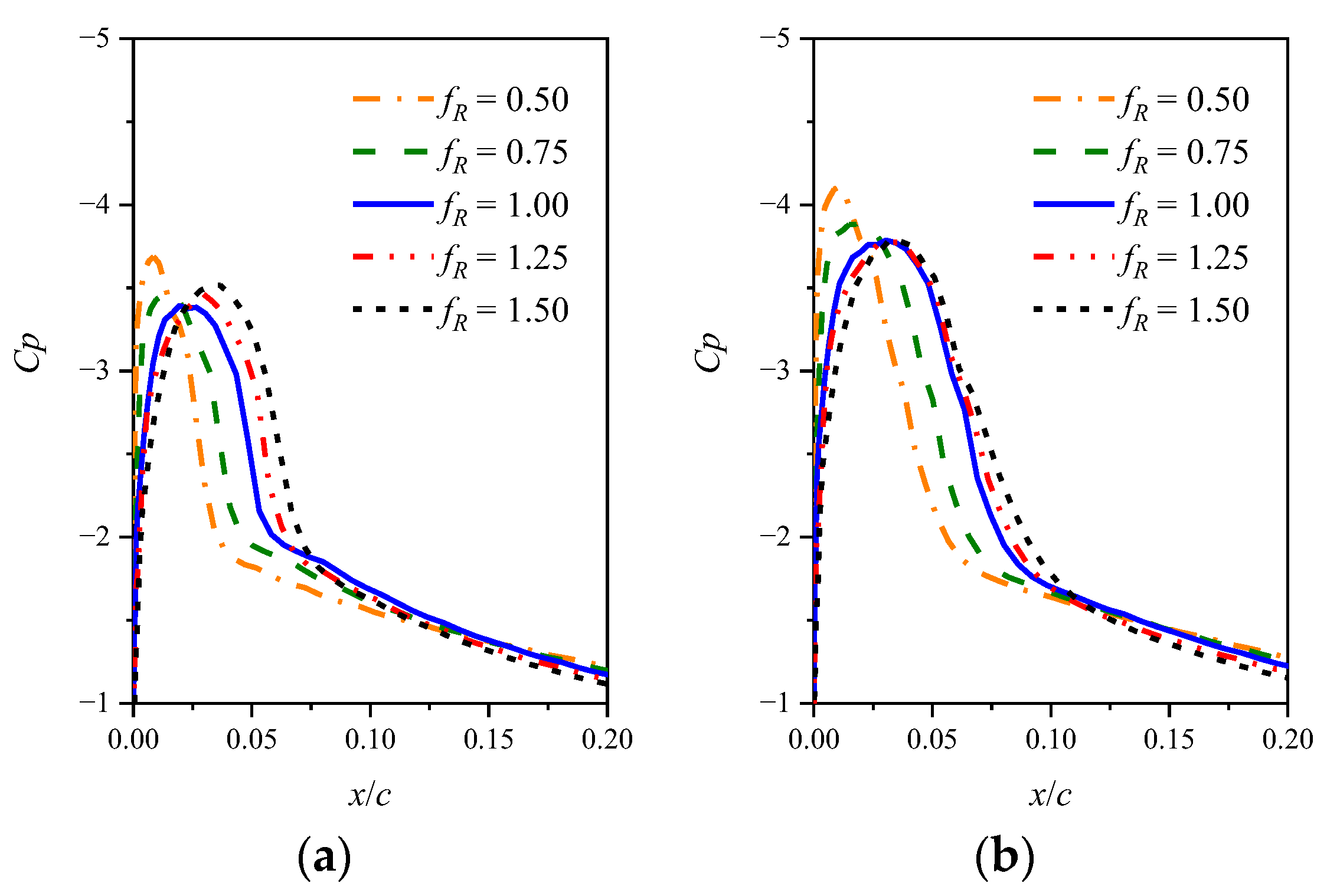
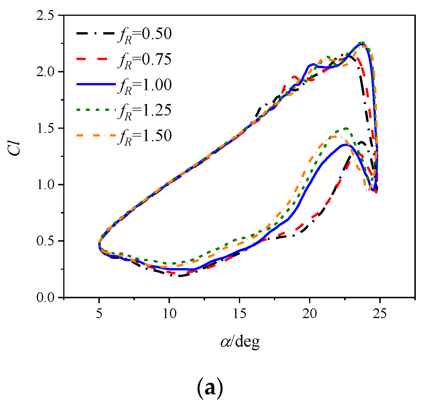
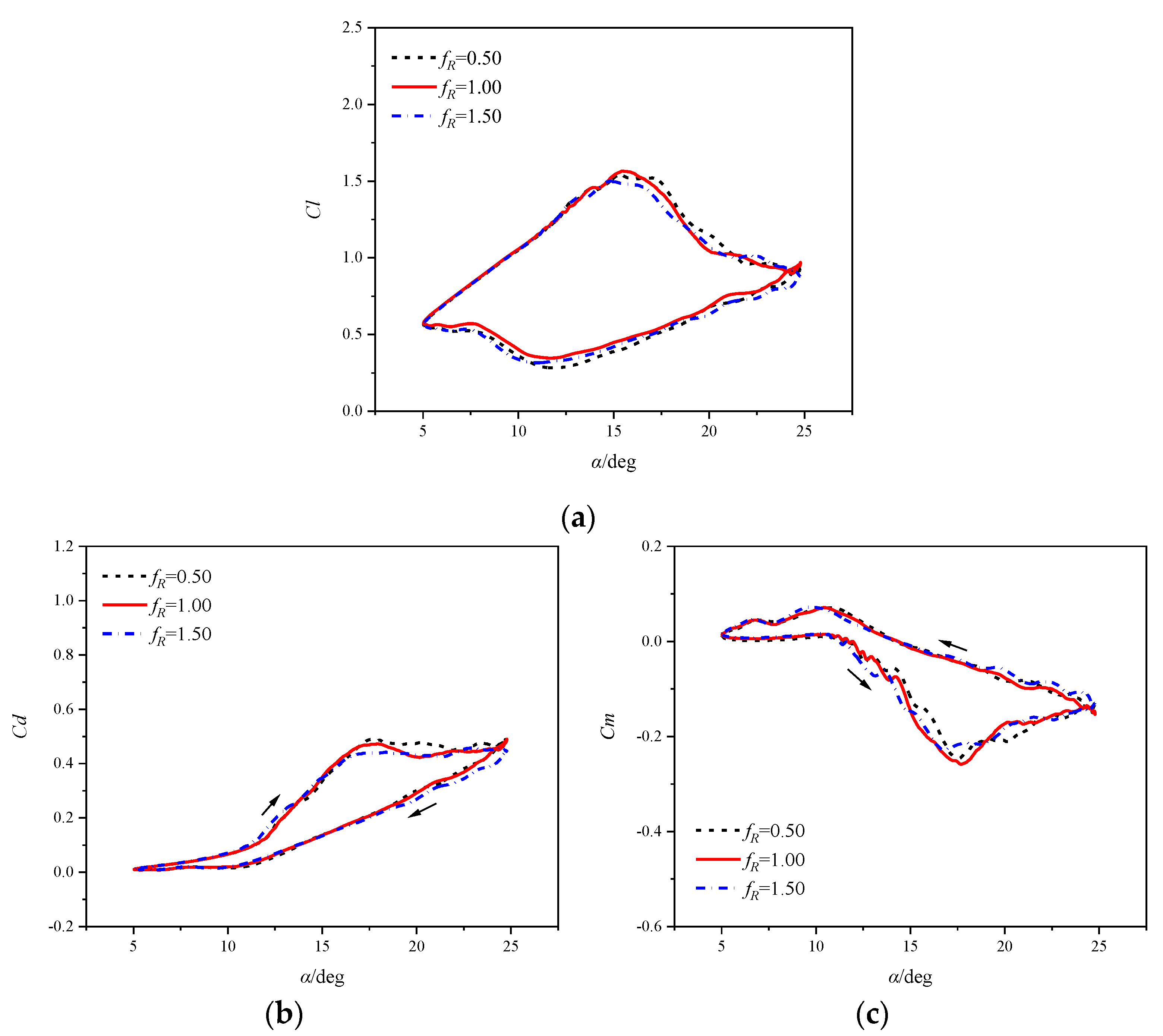
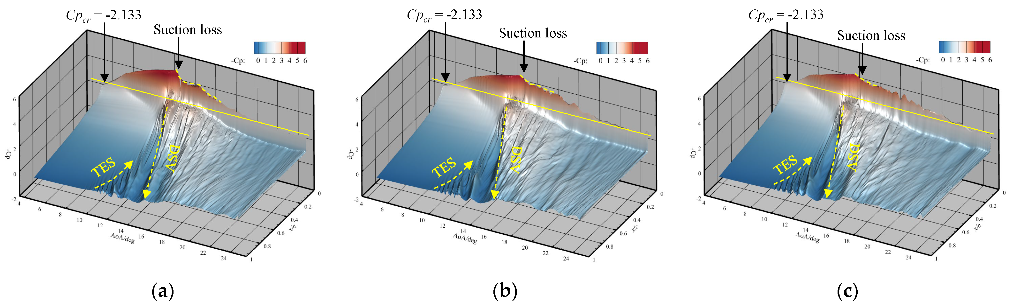
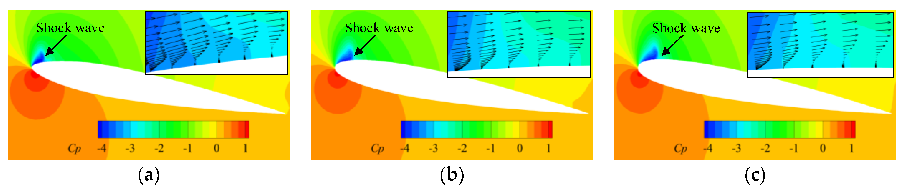
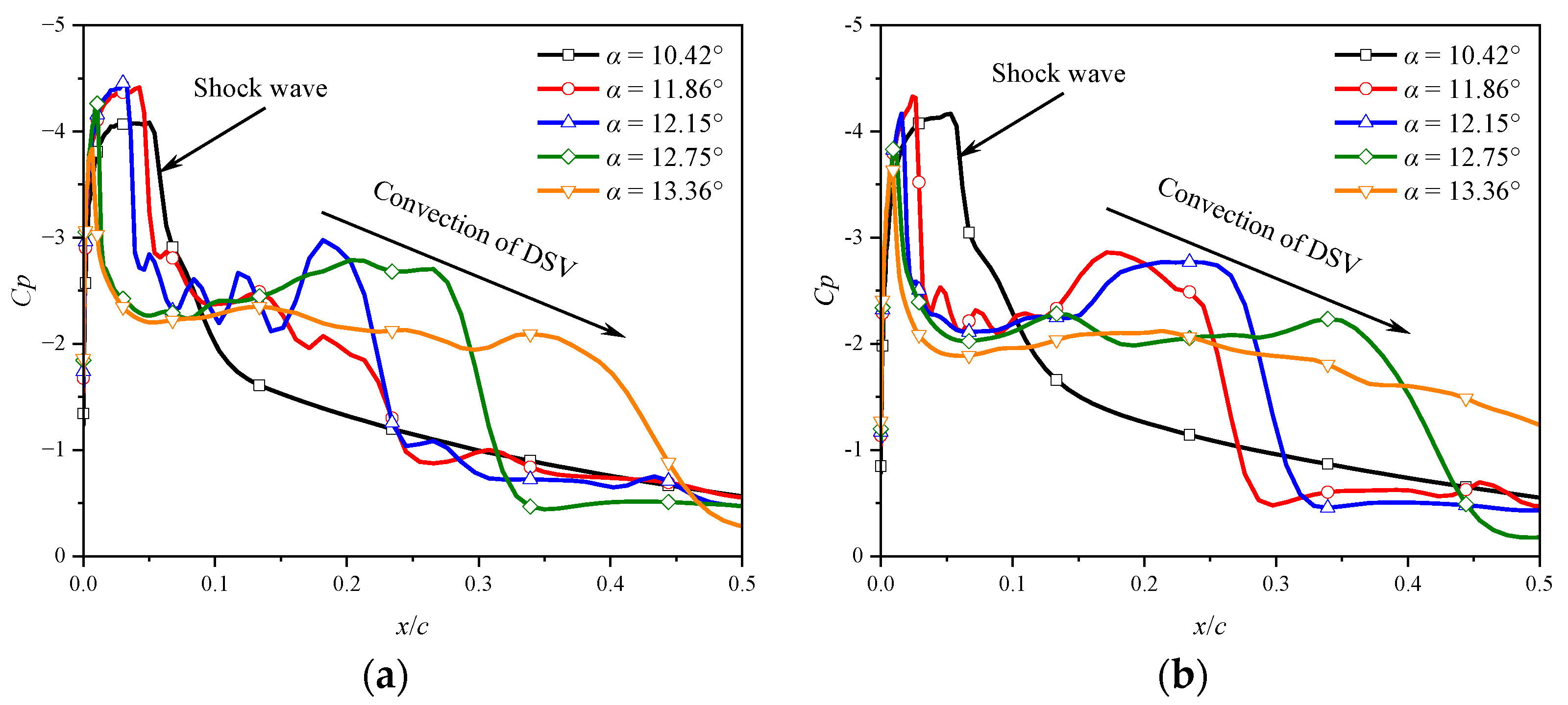
At a high Mach number of 0.5, the airfoil encounters a moderate leading edge stall in both static and dynamic cases. Due to the significant compressibility effects, a shock wave forms near the leading edge and the high adverse pressure gradient near the shock wave induces flow separation. Instead of a collapse of the suction pressure peak, the shock-induced separation expands and causes a gradual decrease in the suction pressure peak, resulting in a smooth variation in aerodynamic loads. Increasing the leading edge radius reduces the compressibility effects, weakens the shock wave and shifts the shock wave aft on the chord, but has minimal effects on the adverse pressure gradient near the shock wave. Consequently, variations in the leading edge radius have minimal effects on the shock-induced stall characteristics.

References

1. Leishmann, J.G. Principles of Helicopter Aerodynamics; Cambridge University Press: New York, NY, USA, 2006. [Google Scholar]
2. McCroskey, W.J.; Carr, L.W.; McAlister, K.W. Dynamic Stall Experiments on Oscillating Airfoils. AIAA J. 1976, 14, 57–63. [Google Scholar] [CrossRef]
3. Carr, L.W.; McAlister, K.W.; McCroskey, W.J. Analysis of the Development of Dynamic Stall Based on Oscillating Airfoil Experiments. NASA TN D-8382, 1 January 1977. [Google Scholar]
4. McCroskey, W.J.; McAlister, K.W.; Carr, L.W.; Pucci, S.L.; Lambert, O.; Indergrand, R.F. Dynamic Stall on Advanced Airfoil Sections. J. Am. Helicopter Soc. 1981, 26, 40–50. [Google Scholar] [CrossRef]
5. Noonan, K.W.; Bingham, G.J. Aerodynamic Characteristics of Three Helicopter Rotor Airfoil Sections at Reynolds Number from Model Scale to Full Scale at Mach Numbers from 0.35 to 0.90. NASA-TP-1701, 1 September 1980. [Google Scholar]
6. Benton, S.I.; Visbal, M.R. Effects of Compressibility on Dynamic-Stall Onset Using Large-Eddy Simulation. AIAA J. 2020, 58, 1194–1205. [Google Scholar] [CrossRef]
7. Fung, K.Y.; Carr, L.W. Effects of Compressibility on Dynamic Stall. AIAA J. 1991, 29, 306–308. [Google Scholar] [CrossRef]
8. Carr, L.W.; Chandrasekhara, M.S. Compressibility effects on dynamic stall. Prog. Aerosp. Sci. 1996, 32, 523–573. [Google Scholar] [CrossRef]
9. Kim, T.; Kim, S.; Lim, J.; Jee, S. Numerical Investigation of Compressibility Effect on Dynamic Stall. Aerosp. Sci. Technol. 2020, 105, 105918. [Google Scholar] [CrossRef]
10. Jacobs, E.N.; Sherman, A. Airfoil Section Characteristics as Affected by Variations of the Reynolds Number. NACA-TR-586, 1 January 1937. [Google Scholar]
11. Kiefer, J.; Brunner, C.E.; Hansen, M.O.L.; Hultmark, M. Dynamic Stall at High Reynolds Numbers Induced by Ramp-Type Pitching Motions. J. Fluid Mech. 2022, 938, A10. [Google Scholar] [CrossRef]
12. Zhu, W.; Bons, J.P.; Gregory, J.W. Reynolds Scaling Effects on Dynamic Stall of VR-7 and VR-12 Airfoils. In Proceedings of the AIAA Scitech 2019 Forum, San Diego, CA, USA, 7–11 January 2019. [Google Scholar]
13. McCroskey, W.J. The Phenomenon of Dynamic Stall. NASA TM-81264, 1 March 1981. [Google Scholar]
14. Choudhuri, P.G.; Knight, D.D. Effects of compressibility, pitch rate, and Reynolds number on unsteady incipient leading-edge boundary layer separation over a pitching airfoil. J. Fluid Mech. 1996, 308, 195–217. [Google Scholar] [CrossRef]
15. McCroskey, W.J.; McAlister, K.W.; Carr, L.W.; Pucci, S.L. An Experimental Study of Dynamic Stall on Advanced Airfoil Sections Volume 1. Summary of the Experiment. NASA-TM-84245, 1 July 1982. [Google Scholar]
16. McAlister, K.W.; Pucci, S.L.; McCroskey, W.J.; Carr, L.W. An Experimental Study of Dynamic Stall on Advanced Airfoil Sections Volume 2. Pressure and Force Data. NASA-TM-84245, 1 September 1982. [Google Scholar]
17. Carr, L.W.; McCroskey, W.J.; McAlister, K.W.; Pucci, S.L.; Lambert, O. An Experimental Study of Dynamic Stall on Advanced Airfoil Sections Volume 3. Hot-Wire and Hot-Film Measurements. NASA-TM-84245, 1 December 1982. [Google Scholar]
18. Sharma, A.; Visbal, M. Numerical Investigation of the Effect of Airfoil Thickness on Onset of Dynamic Stall. J. Fluid Mech. 2019, 870, 870–900. [Google Scholar] [CrossRef]
19. Shum, J.G.; Lee, S. Effect of Airfoil Design Parameters on Deep Dynamic Stall under Pitching Motion. In Proceedings of the AIAA SciTech 2023 Forum, National Harbor, MD, USA, 23–27 January 2023. [Google Scholar]
20. Ekaterinaris, J.A. Numerical investigations of dynamic stall active control for incompressible and compressible flows. J. Aircr. 2002, 39, 71–78. [Google Scholar] [CrossRef]
21. Müller-Vahl, H.F.; Strangfeld, C.; Nayeri, C.N.; Paschereit, C.O.; Greenblatt, D. Control of Thick Airfoil, Deep Dynamic Stall Using Steady Blowing. Aiaa J. 2015, 53, 277–295. [Google Scholar] [CrossRef]
22. Rehman, A.; Kontis, K. Synthetic Jet Control Effectiveness on Stationary and Pitching Airfoils. J. Aircr. 2006, 43, 1782–1789. [Google Scholar] [CrossRef]
23. Martin, P.B.; McAlisterK, W.; Chandrasekhara, M.S.; Geissler, W. Dynamic stall measurements and computations for a VR-12 airfoil with a variable droop leading edge. In Proceedings of the AHS International Forum 59, Phoenix, AZ, USA, 6–8 May 2003.
24. Chandrasekhara, M.S.; Martin, P.B.; Tung, C. compressible dynamic stall control using a variable droop leading edge airfoil. J. Aircr. 2012, 41, 862–869. [Google Scholar] [CrossRef]
25. Hassan, A.A.; Straub, F.K.; Noonan, K.W. Experimental/Numerical Evaluation of Integral Trailing Edge Flaps for Helicopter Rotor Applications. J. Am. Helicopter Soc. 2005, 50, 3–17. [Google Scholar] [CrossRef]
26. Tang, J.W.; Hu, Y.; Song, B.F.; Yang, H. Unsteady Aerodynamic Optimization of Airfoil for Cycloidal Propellers Based on Surrogate Model. J. Aircr. 2017, 54, 1241–1256. [Google Scholar] [CrossRef]
27. Wang, Q.; Zhao, Q.J. Rotor Airfoil Profile Optimization for Alleviating Dynamic Stall Characteristics. Aerosp. Sci. Technol. 2018, 72, 502–515. [Google Scholar] [CrossRef]
28. Jing, S.M.; Zhao, Q.J.; Zhao, G.Q.; Wang, Q. Multi-Objective Airfoil Optimization Under Unsteady-Freestream Dynamic Stall Conditions. J. Aircr. 2023, 60, 293–309. [Google Scholar] [CrossRef]
29. Lim, J.W. Application of Parametric Airfoil Design for Rotor Performance Improvement. In Proceedings of the 44th European Rotrocraft Forum, Delft, The Netherlands, 18–21 September 2018. [Google Scholar]
30. Zhao, Q.J.; Zhao, G.Q.; Wang, B.; Wang, Q.; Shi, Y.J.; Xu, G.H. Robust Navier-Stokes Method for Predicting Unsteady Flowfield and Aerodynamic Characteristics of Helicopter Rotor. Chin. J. Aeronaut. 2018, 31, 214–224. [Google Scholar] [CrossRef]
31. Gritskevich, M.S.; Garbaruk, A.V.; Schutze, J.; Menter, F.R. Development of DDES and IDDES Formulations for the k-ω Shear Stress Transport Model. Flow Turbul. Combust. 2012, 88, 431–449. [Google Scholar] [CrossRef]
32. Travin, A.; Shur, M.; Strelets, M.; Spalart, P. Detached-Eddy Simulations past a Circular Cylinder. Flow Turbul. Combust. 2000, 63, 293–313. [Google Scholar] [CrossRef]
33. Khalifa, N.M.; Rezaei, A.; Taha, H.E. On Computational Simulations of Dynamic Stall and Its Three-Dimensional Nature. Phys. Fluids 2023, 35, 105143. [Google Scholar] [CrossRef]
Figure 1. Comparison of airfoil geometries with different leading edge radii.
Aerospace 11 00470 g001
Figure 2. Comparison of the numerical and experimental airloads [15] of NACA 0012 airfoil at Ma = 0.3: (a) Cl; (b) Cd; (c) Cm.
Aerospace 11 00470 g002
Figure 3. Grid arrangement around the NACA 0012 airfoil.
Aerospace 11 00470 g003
Figure 4. Comparison of the numerical results with different time steps: (a) Cl; (b) Cd; (c) Cm.
Aerospace 11 00470 g004aAerospace 11 00470 g004b
Figure 5. Comparison between the numerical and experimental airloads [16]: (a) Cl; (b) Cd; (c) Cm.
Aerospace 11 00470 g005
Figure 6. Aerodynamic force coefficient of airfoils at Ma = 0.283: (a) Cl; (b) Cd; (c) Cm.
Aerospace 11 00470 g006
Figure 7. Skin friction and pressure coefficient of the airfoil with fR = 0.50: (a) Cf; (b) Cp.
Aerospace 11 00470 g007
Figure 8. Skin friction and pressure coefficient of the airfoil with fR = 1.00: (a) Cf; (b) Cp.
Aerospace 11 00470 g008
Figure 9. Skin friction and pressure coefficient of the airfoil with fR = 1.50: (a) Cf; (b) Cp.
Aerospace 11 00470 g009
Figure 10. Cp contours and streamlines of the airfoil with fR = 0.50: (a) α = 11°; (b) α = 12°.
Aerospace 11 00470 g010
Figure 11. Cp contours and streamlines of the airfoil with fR = 1.00: (a) α = 14°; (b) α = 15°.
Aerospace 11 00470 g011
Figure 12. Cp contours and streamlines of the airfoil with fR = 1.50: (a) α = 14°; (b) α = 15°.
Aerospace 11 00470 g012
Figure 13. The minimum pressure coefficient of airfoils versus AoA.
Aerospace 11 00470 g013
Figure 14. Pressure coefficient distributions of airfoils: (a) α = 2°; (b) α = 8°.
Aerospace 11 00470 g014
Figure 15. Aerodynamic force coefficient of airfoils at Ma = 0.5: (a) Cl; (b) Cd; (c) Cm.
Aerospace 11 00470 g015aAerospace 11 00470 g015b
Figure 16. Pressure coefficients and skin frictions of the NACA 0012 airfoil: (a) Cp; (b) Cf.
Aerospace 11 00470 g016
Figure 17. Pressure coefficient contours and velocity profiles near the shock: (a) α = 7°; (b) α = 8°.
Aerospace 11 00470 g017
Figure 18. Contours of pressure coefficient and streamlines of the NACA 0012 airfoil: (a) α = 11°; (b) α = 12°; (c) α = 13°.
Aerospace 11 00470 g018
Figure 19. Pressure coefficients and skin frictions of the airfoil with fR = 1.50: (a) Cp; (b) Cf.
Aerospace 11 00470 g019
Figure 20. Pressure coefficients near the leading edge of airfoils: (a) α = 7°; (b) α = 8°.
Aerospace 11 00470 g020
Figure 21. Aerodynamic force coefficients of airfoils at Ma = 0.283: (a) Cl; (b) Cd; (c) Cm.
Aerospace 11 00470 g021aAerospace 11 00470 g021b
Figure 22. Effect of leading edge radius on the stall characteristics of airfoils at Ma = 0.283: (a) Stall angle; (b) Peak value of force coefficient.
Aerospace 11 00470 g022
Figure 23. Contours of spanwise averaged pressure coefficient for airfoils during the pitching-up process at Ma = 0.283: (a) fR = 0.50; (b) fR = 1.00; (c) fR = 1.50.
Aerospace 11 00470 g023
Figure 24. Distributions of spanwise averaged skin friction of airfoils before the collapse of suction pressure peak.
Aerospace 11 00470 g024
Figure 25. Distributions of spanwise averaged pressure coefficient near the leading edge of airfoils: (a) Cp near the collapse of suction pressure peak; (b) Cp at α = 15.22°.
Aerospace 11 00470 g025
Figure 26. Aerodynamic force coefficients of airfoils at Ma = 0.5: (a) Cl; (b) Cd; (c) Cm.
Aerospace 11 00470 g026
Figure 27. Contours of spanwise averaged pressure coefficient for airfoils during the pitching-up process at Ma = 0.5: (a) fR = 0.50; (b) fR = 1.00; (c) fR = 1.50.
Aerospace 11 00470 g027
Figure 28. Spanwise averaged pressure coefficients near the leading edge: (a) α = 9.10°; (b) α = 10.42°.
Aerospace 11 00470 g028
Figure 29. Contours of pressure coefficient and velocity profiles of the central cross-section at α = 10.42°: (a) fR = 0.50; (b) fR = 1.00; (c) fR = 1.50.
Aerospace 11 00470 g029
Figure 30. Spanwise averaged pressure coefficients in the pitching-up circle: (a) fR = 1.00; (b) fR = 1.50.
Aerospace 11 00470 g030
Figure 31. Iso-surface of Q criterion of the NACA 0012 airfoil at α = 13.36° (Q = 200).
Aerospace 11 00470 g031