
Numerical Study on the Cooling Method of Phase Change Heat Exchange Unit with Layered Porous Media


Abstract
:1. Introduction
2. Methodology
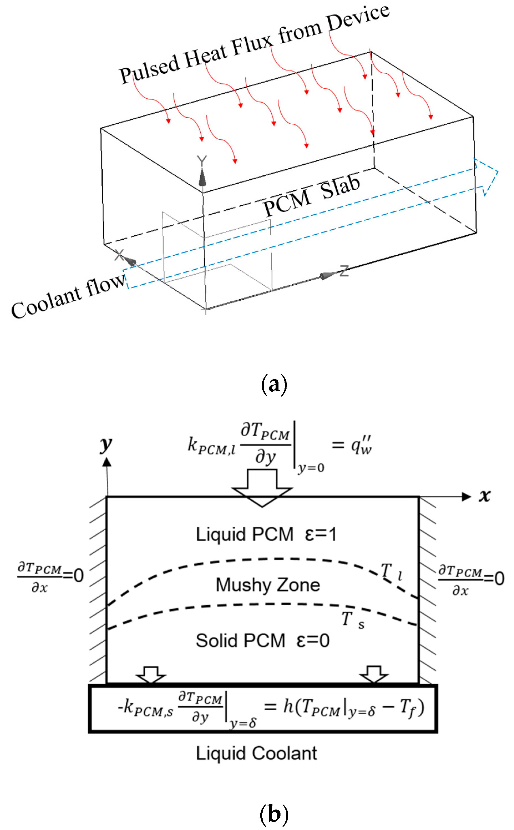
2.1. Physical Model
2.2. Control Equations and Thermal Boundary Conditions
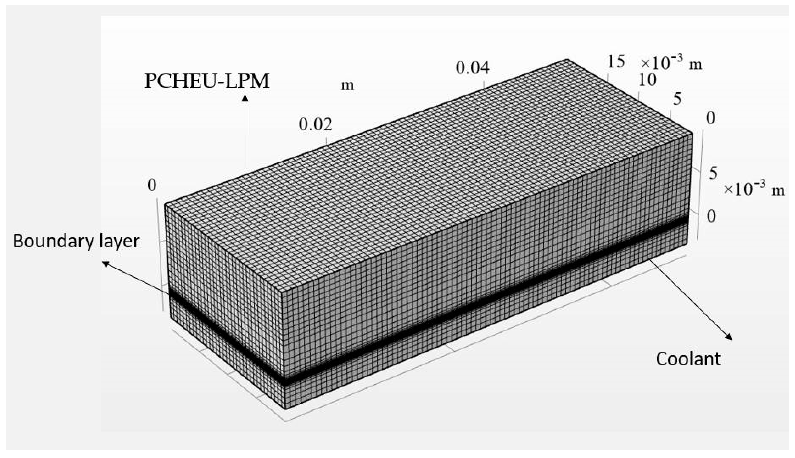
2.3. Solving Methods
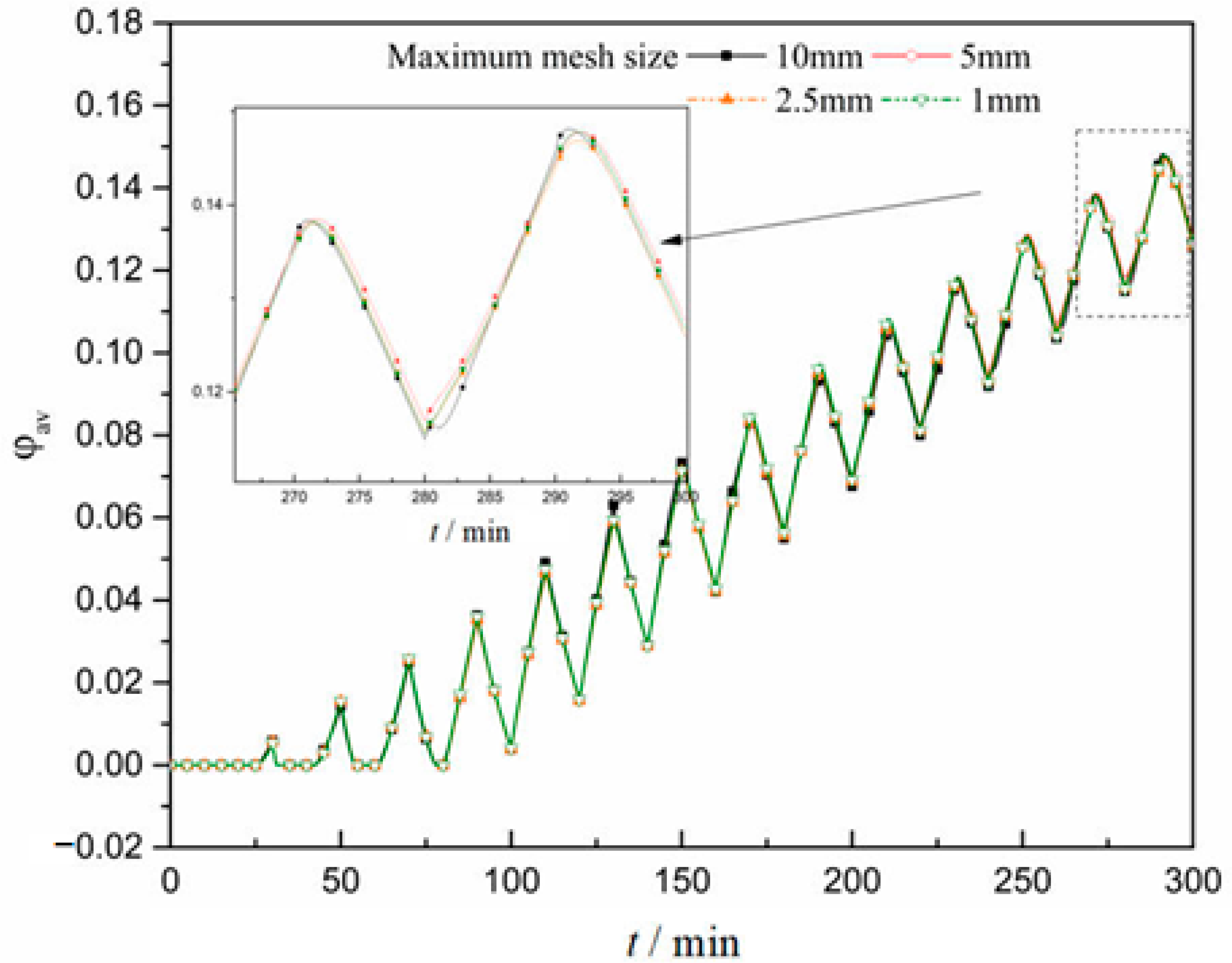
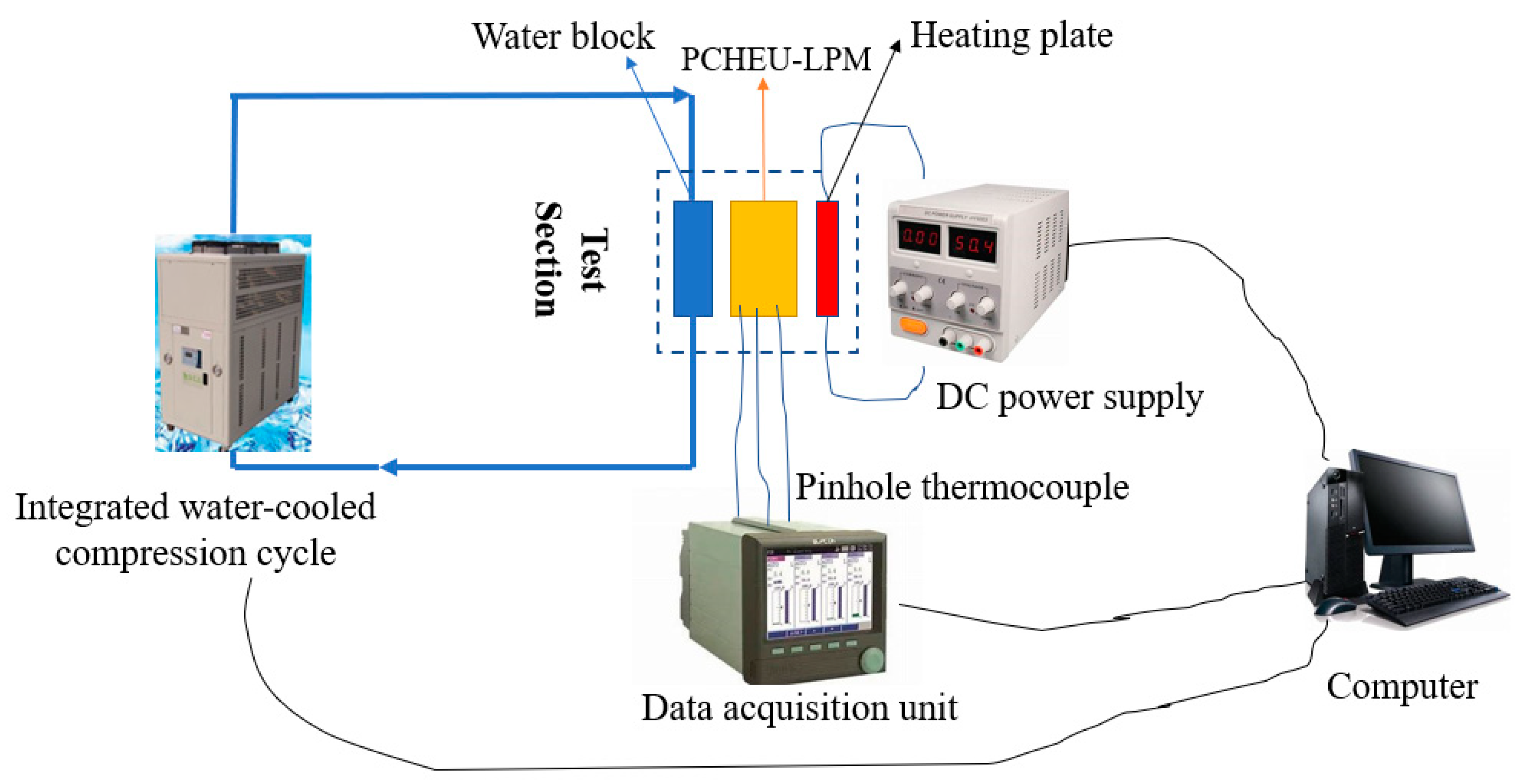
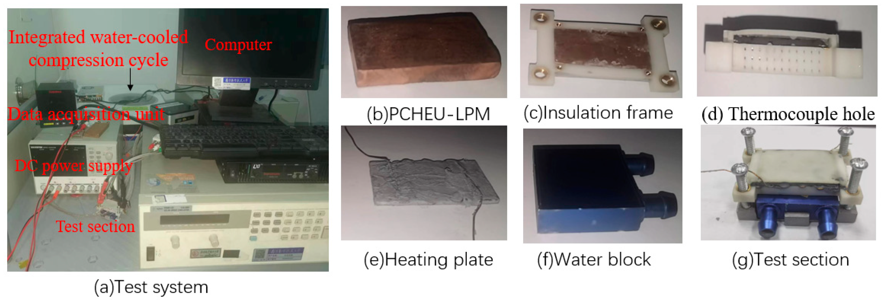
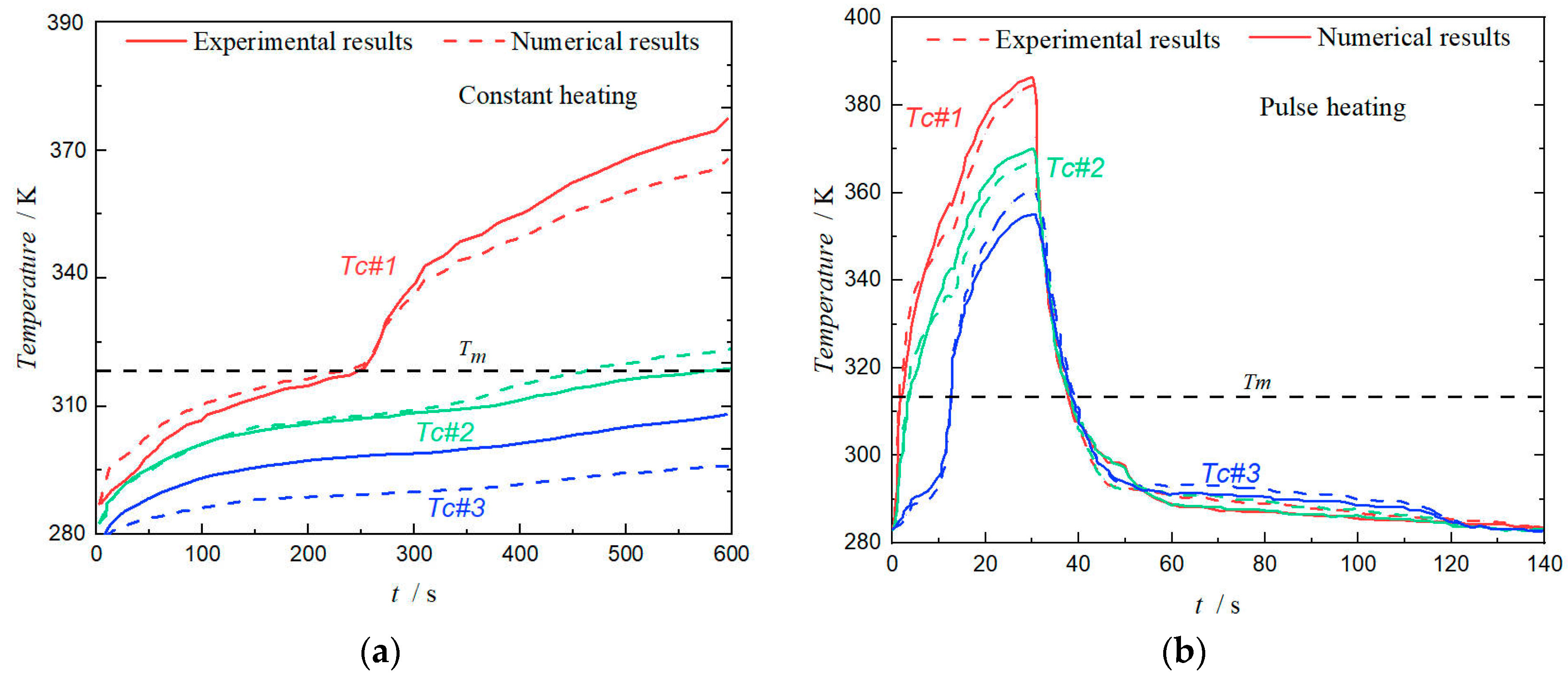
2.4. Model Validation
3. Simulation Results and Discussion
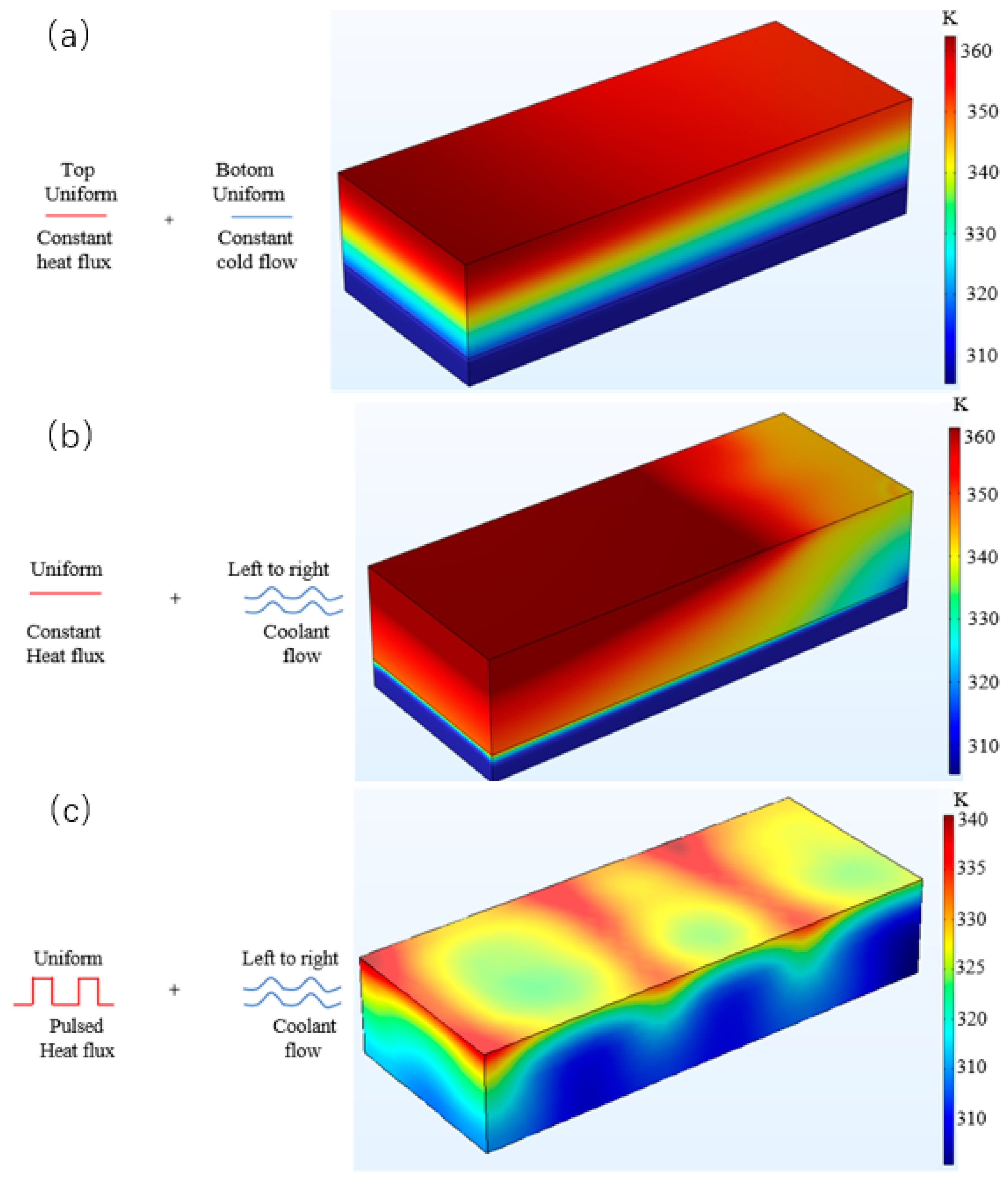
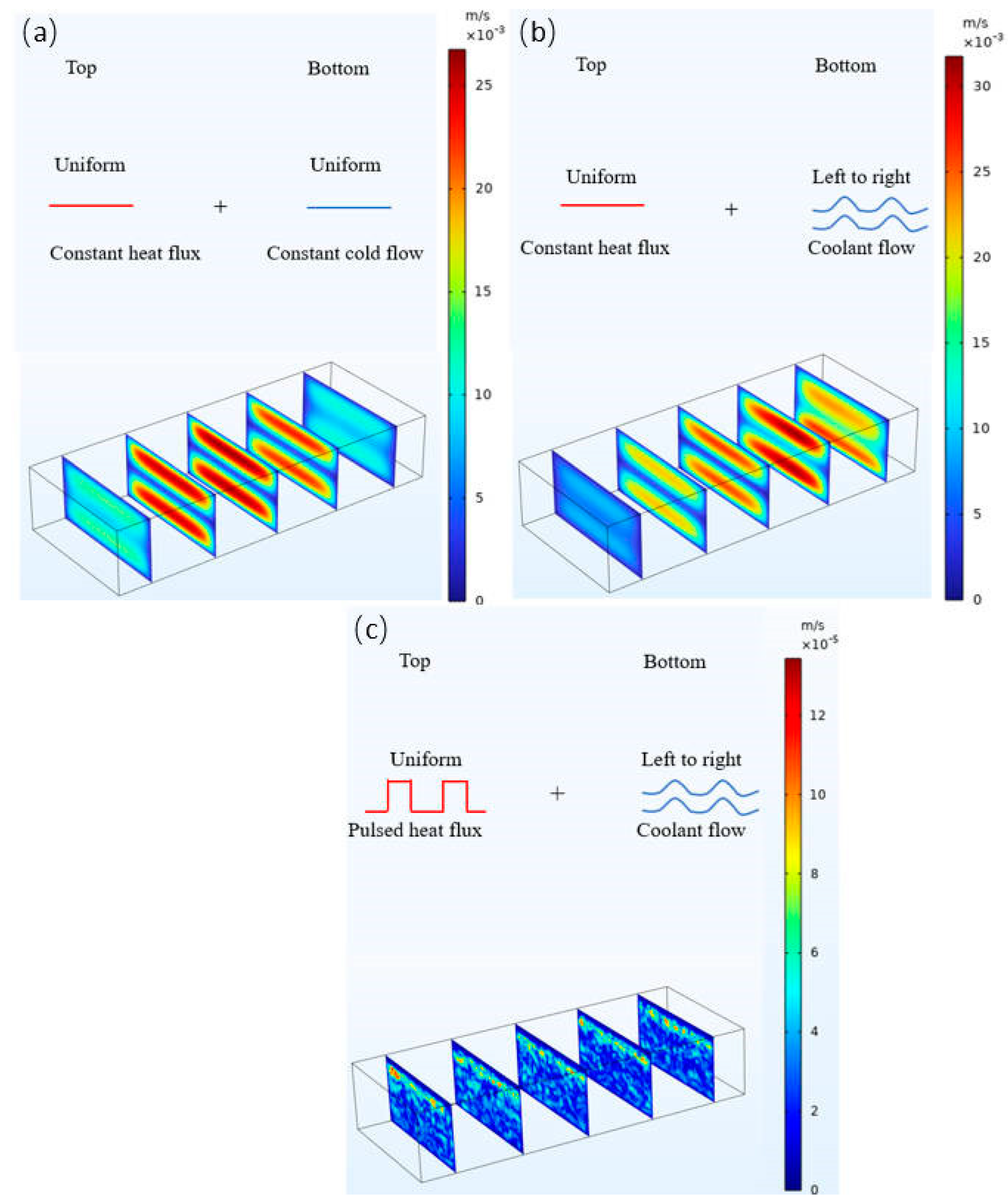
3.1. Influence of Thermal Boundary Conditions on Temperature and Velocity Fields
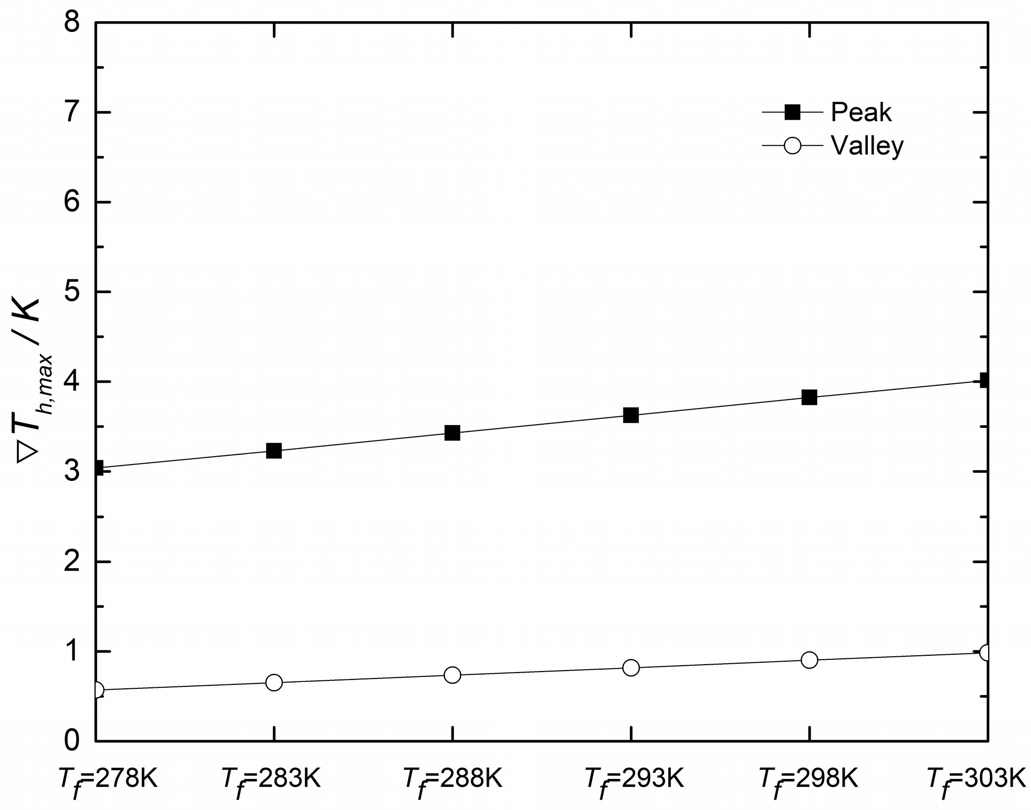
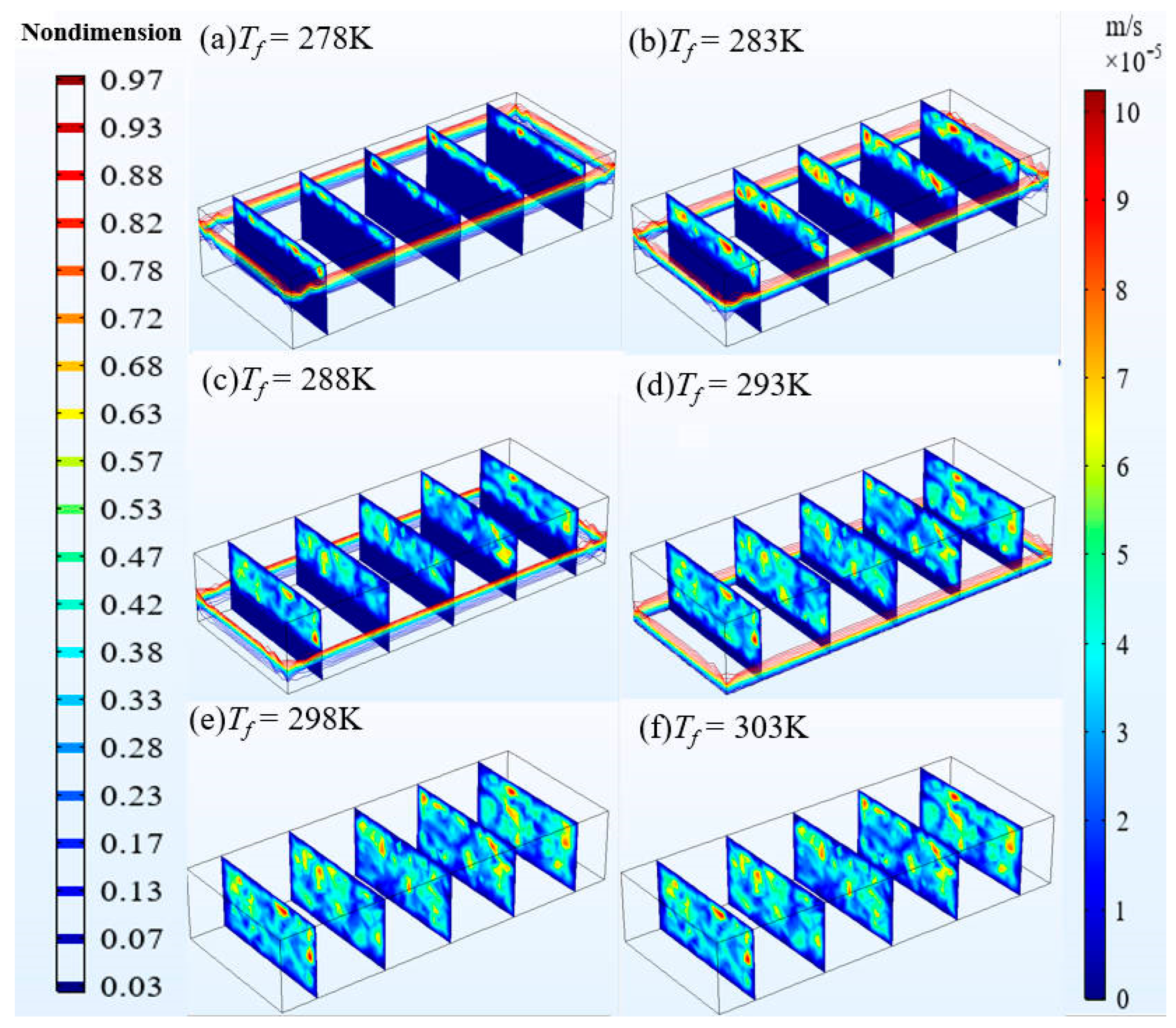
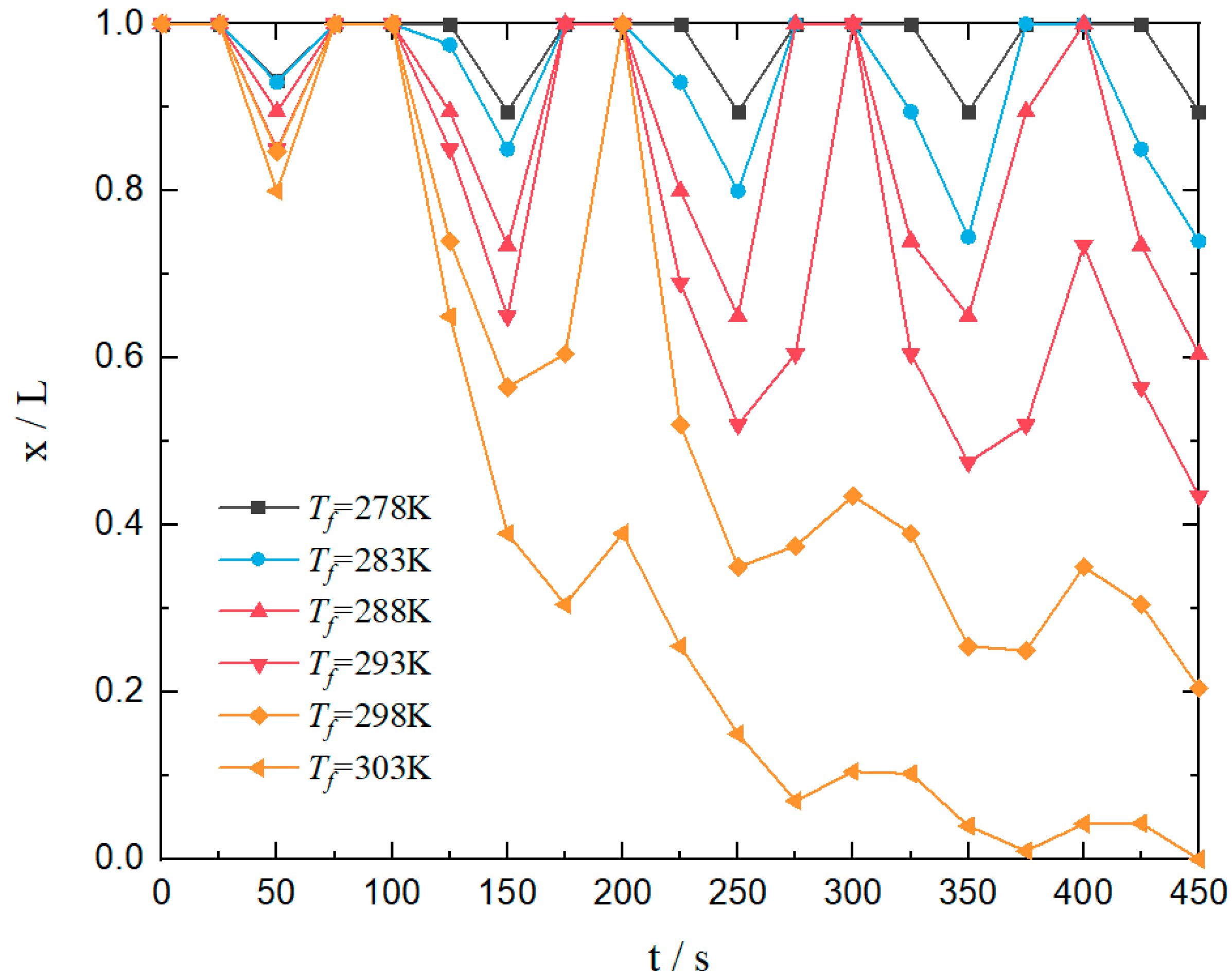
3.2. Thermal Response of Incoming Flow Temperature
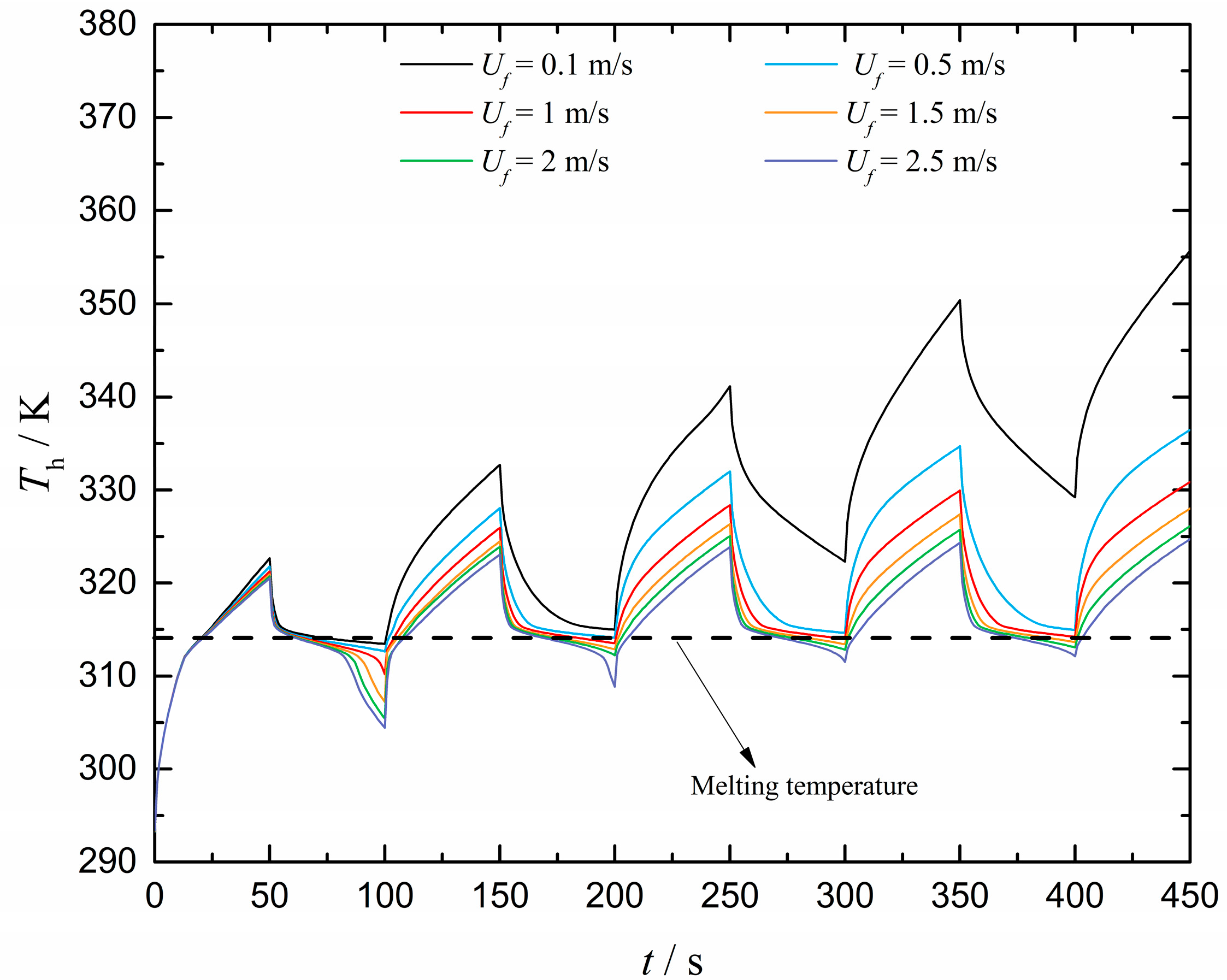
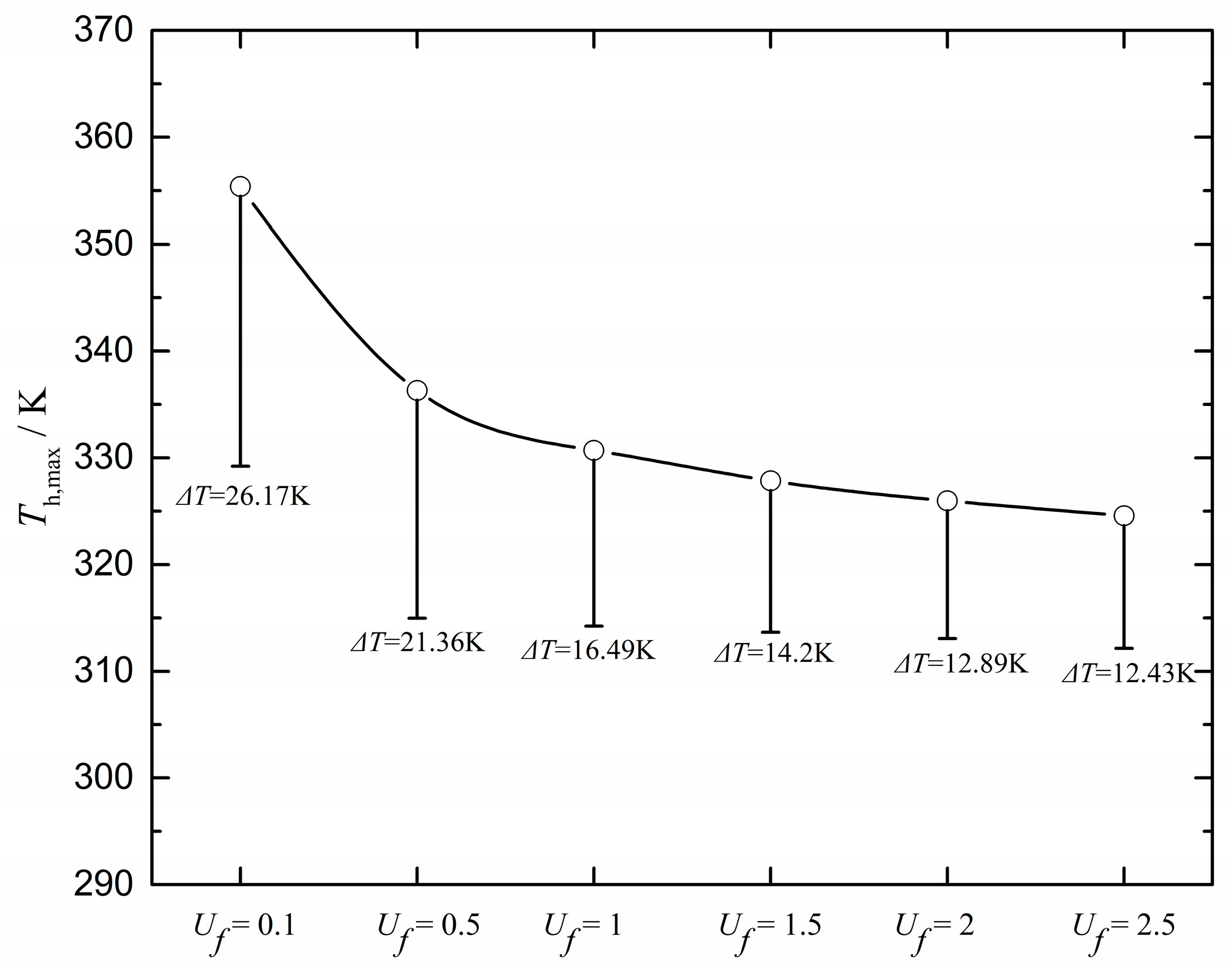
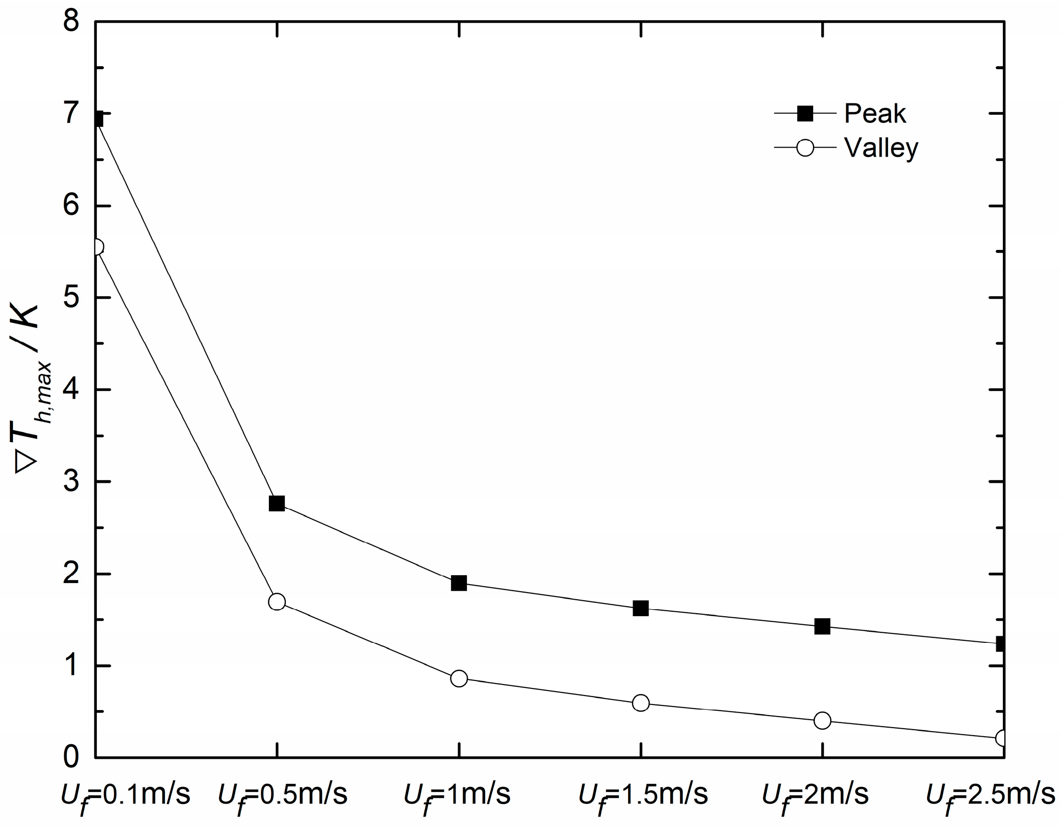
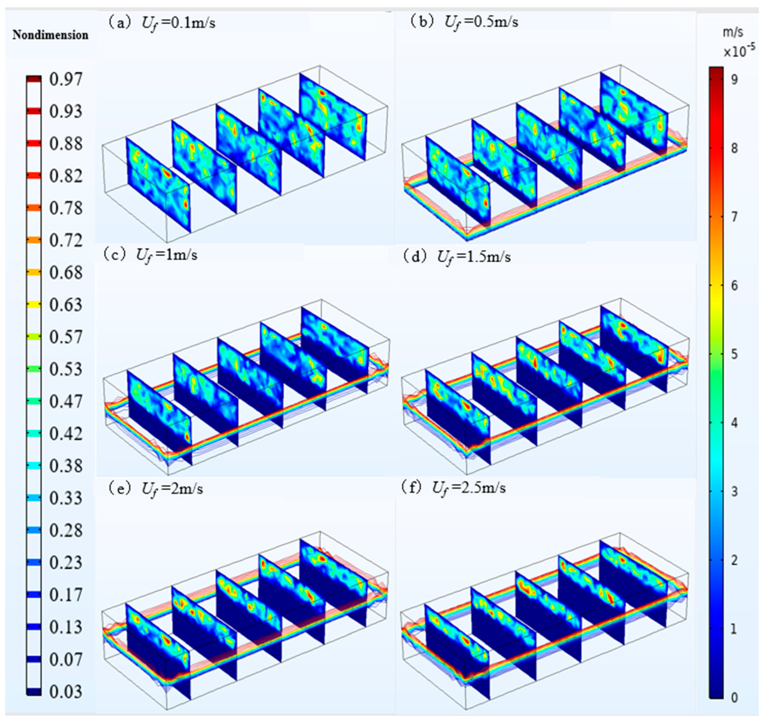
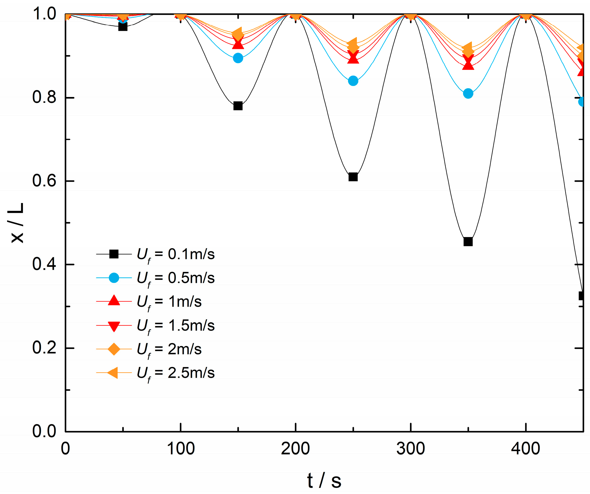
3.3. Thermal Response of Incoming Flow Velocity
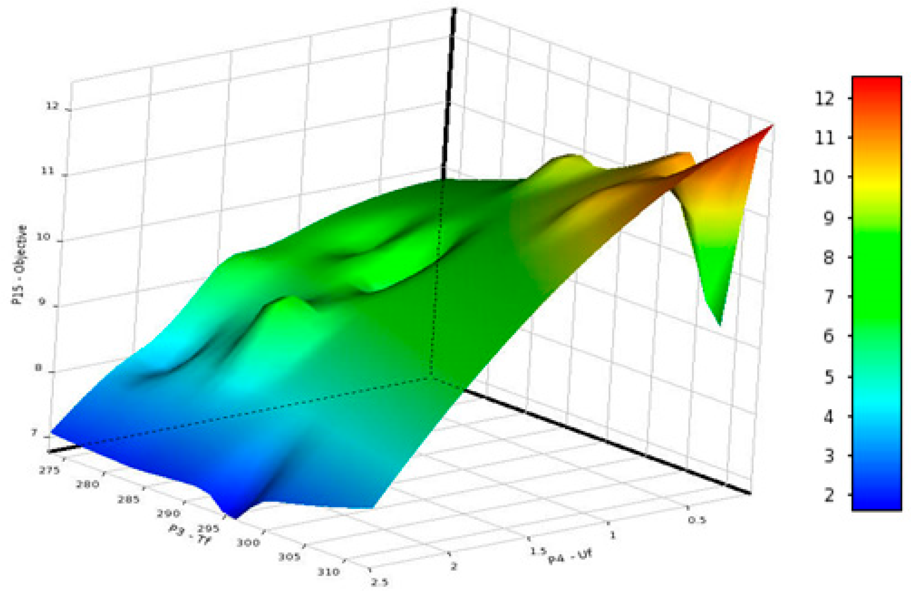
3.4. Method for Solving Optimal Values
4. Conclusions
Author Contributions
Funding
Data Availability Statement
Conflicts of Interest
Nomenclature
| Parameter name | ||
| Length | mm | |
| Width | mm | |
| Height | mm | |
| Heat flow | W/m2 | |
| Temperature | K | |
| X-direction speed | m/s | |
| Y-direction speed | m/s | |
| Z-direction speed | m/s | |
| Body-force | N/m3 | |
| S | Phase interface location | m |
| Convective heat transfer coefficient | W/m2-K | |
| Δh | Latent heat of phase change | KJ/kg |
| Greek alphabet | ||
| Time | s | |
| Porosity or liquid phase ratio | ||
| Sport viscosity | Pa-s | |
| Density | Kg/m3 | |
| Thermal conductivity | W/m-k | |
| Latent heat of phase change | KJ/kg | |
| Thermal diffusion coefficient | m2/s | |
| Liquid fraction | ||
| Subscript | ||
| L | Liquid phase | |
| Solid phase | ||
| Directional vector at the phase interface | ||
| W | External thermal excitation | |
| M | Phase change state | |
| C | Cold fluids | |
| 0 | Initial state | |
| Ss | Steady state, time-averaged value of transient temperature fluctuations | |
| Abbreviation | ||
| PCHEU-LPM | Phase Change Heat Exchange Unit with Layered Porous Media | |
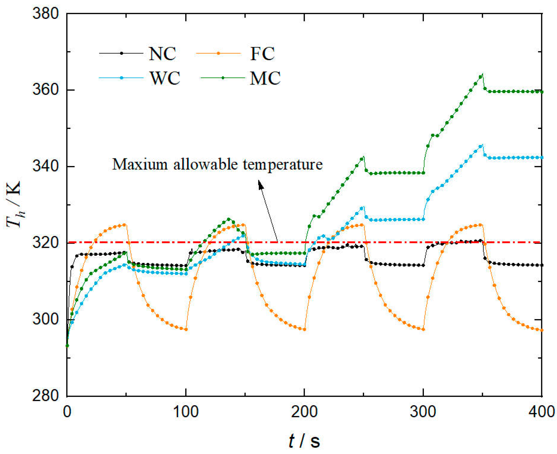
| NC | Natural cooling | |
| FC | Fan cooling | |
| WC | Water cooling | |
| MC | Microchannel cooling |
References
- Gou, J.; Xiao, S.; Hu, J.; Gao, G.; Gong, C. Research Progress of Aerodynamic Heat Dissipation, Transport and Conversion Technologies of Hypersonic Vehicles. Yuhang Xuebao/J. Astronaut. 2022, 43, 983–999. [Google Scholar] [CrossRef]
- Behrens, B.; Müller, M. Technologies for Thermal Protection Systems Applied on Re-Usable Launcher. Acta Astronaut. 2004, 55, 529–536. [Google Scholar] [CrossRef]
- Gori, F.; Corasaniti, S.; Worek, W.M.; Minkowycz, W.J. Theoretical Prediction of Thermal Conductivity for Thermal Protection Systems. Appl. Therm. Eng. 2012, 49, 124–130. [Google Scholar] [CrossRef]
- Mehta, J.; Charneski, J.; Wells, P. Unmanned Aerial Systems (UAS) Thermal Management Needs, Current Status, and Future Innovations. In Proceedings of the 10th International Energy Conversion Engineering Conference, Atlanta, GA, USA, 30 July–1 August 2012; ISBN 978-1-62410-190-8. [Google Scholar]
- Balland, S.; Fernandez Villace, V.; Steelant, J. Thermal and Energy Management for Hypersonic Cruise Vehicles—Cycle Analysis. In Proceedings of the 20th AIAA International Space Planes and Hypersonic Systems and Technologies Conference, Glasgow, UK, 6–9 July 2015; American Institute of Aeronautics and Astronautics, 2015. [Google Scholar]
- Lee, S.H.; Mudawar, I.; Hasan, M.M. Thermal Analysis of Hybrid Single-Phase, Two-Phase and Heat Pump Thermal Control System (TCS) for Future Spacecraft. Appl. Therm. Eng. 2016, 100, 190–214. [Google Scholar] [CrossRef]
- Guo, W.; Li, Y.; Li, Y.-Z.; Zhong, M.-L.; Wang, S.-N.; Wang, J.-X.; Li, E.-H. An Integrated Hardware-in-the-Loop Verification Approach for Dual Heat Sink Systems of Aerospace Single Phase Mechanically Pumped Fluid Loop. Appl. Therm. Eng. 2016, 106, 1403–1414. [Google Scholar] [CrossRef]
- Waser, R.; Ghani, F.; Maranda, S.; O’Donovan, T.S.; Schuetz, P.; Zaglio, M.; Worlitschek, J. Fast and Experimentally Validated Model of a Latent Thermal Energy Storage Device for System Level Simulations. Appl. Energy 2018, 231, 116–126. [Google Scholar] [CrossRef]
- Maxa, J.; Novikov, A.; Nowottnick, M.; Heimann, M.; Jarchoff, K. Phase Change Materials for Thermal Peak Management Applications with Specific Temperature Ranges. In Proceedings of the 2018 17th IEEE Intersociety Conference on Thermal and Thermomechanical Phenomena in Electronic Systems (ITherm), San Diego, CA, USA, 29 May–1 June 2018; IEEE, 2018; pp. 92–101. [Google Scholar]
- Krishnan, S.; Garimella, S.V. Analysis of a Phase Change Energy Storage System for Pulsed Power Dissipation. IEEE Trans. Comp. Packag. Technol. 2004, 27, 191–199. [Google Scholar] [CrossRef]
- Shamberger, P.J.; Hoe, A.; Deckard, M.; Barako, M.T. Effects of Boundary Conditions on the Dynamic Response of a Phase Change Material. In Proceedings of the 2020 19th IEEE Intersociety Conference on Thermal and Thermomechanical Phenomena in Electronic Systems (ITherm), Orlando, FL, USA, 21–23 July 2020; IEEE, 2020; pp. 985–992. [Google Scholar]
- Kim, T.Y.; Hyun, B.-S.; Lee, J.-J.; Rhee, J. Numerical Study of the Spacecraft Thermal Control Hardware Combining Solid–Liquid Phase Change Material and a Heat Pipe. Aerosp. Sci. Technol. 2013, 27, 10–16. [Google Scholar] [CrossRef]
- Gilmore, D. Spacecraft Thermal Control Handbook; Aerospace Press: Chantilly, VA, USA, 2002; ISBN 978-1-884989-11-7. [Google Scholar]
- Lin, Y.; Jia, Y.; Alva, G.; Fang, G. Review on Thermal Conductivity Enhancement, Thermal Properties and Applications of Phase Change Materials in Thermal Energy Storage. Renew. Sustain. Energy Rev. 2018, 82, 2730–2742. [Google Scholar] [CrossRef]
- Gürel, B. A Numerical Investigation of the Melting Heat Transfer Characteristics of Phase Change Materials in Different Plate Heat Exchanger (Latent Heat Thermal Energy Storage) Systems. Int. J. Heat Mass Transf. 2020, 148, 119117. [Google Scholar] [CrossRef]
- Youssef, W.; Ge, Y.T.; Tassou, S.A. CFD Modelling Development and Experimental Validation of a Phase Change Material (PCM) Heat Exchanger with Spiral-Wired Tubes. Energy Convers. Manag. 2018, 157, 498–510. [Google Scholar] [CrossRef]
- Huang, Z.; Xie, N.; Zheng, X.; Gao, X.; Fang, X.; Fang, Y.; Zhang, Z. Experimental and Numerical Study on Thermal Performance of Wood’s Alloy/Expanded Graphite Composite Phase Change Material for Temperature Control of Electronic Devices. Int. J. Therm. Sci. 2019, 135, 375–385. [Google Scholar] [CrossRef]
- Fan, L.-W.; Xiao, Y.-Q.; Zeng, Y.; Fang, X.; Wang, X.; Xu, X.; Yu, Z.-T.; Hong, R.-H.; Hu, Y.-C.; Cen, K.-F. Effects of Melting Temperature and the Presence of Internal Fins on the Performance of a Phase Change Material (PCM)-Based Heat Sink. Int. J. Therm. Sci. 2013, 70, 114–126. [Google Scholar] [CrossRef]
- Zhou, J.; Cao, X.; Zhang, N.; Yuan, Y.; Zhao, X.; Hardy, D. Micro-Channel Heat Sink: A Review. J. Therm. Sci. 2020, 29, 1431–1462. [Google Scholar] [CrossRef]
- Mazzeo, D.; Oliveti, G.; De Simone, M.; Arcuri, N. Analytical Model for Solidification and Melting in a Finite PCM in Steady Periodic Regime. Int. J. Heat Mass Transf. 2015, 88, 844–861. [Google Scholar] [CrossRef]


| Name of Material | Thermal Conductivity (W/m-K) | Density (kg/m3) | Specific Heat Capacity (J/kg-K) | Latent Heat (kJ/kg) | Melting Temperature(K) |
|---|---|---|---|---|---|
| Paraffin | 0.558 | 900 | 2170 | 220 | 323 |
| Copper foam | 385 | 7900 | 3900 | / | / |
| Parameter Name | Value | Maximum Temperature | Temperature Fluctuation |
|---|---|---|---|
| k | 15.53 (W/mK) | 313.2 K | 11.5 K |
| L | 0.042 m | ||
| Tf | 296 K | ||
| Uf | 2.5 m/s |
Disclaimer/Publisher’s Note: The statements, opinions and data contained in all publications are solely those of the individual author(s) and contributor(s) and not of MDPI and/or the editor(s). MDPI and/or the editor(s) disclaim responsibility for any injury to people or property resulting from any ideas, methods, instructions or products referred to in the content. |
© 2024 by the authors. Licensee MDPI, Basel, Switzerland. This article is an open access article distributed under the terms and conditions of the Creative Commons Attribution (CC BY) license (https://creativecommons.org/licenses/by/4.0/).
Share and Cite
Zhang, R.-J.; Zhang, J.-Y.; Zhang, J.-Z. Numerical Study on the Cooling Method of Phase Change Heat Exchange Unit with Layered Porous Media. Aerospace 2024, 11, 487. https://doi.org/10.3390/aerospace11060487
Zhang R-J, Zhang J-Y, Zhang J-Z. Numerical Study on the Cooling Method of Phase Change Heat Exchange Unit with Layered Porous Media. Aerospace. 2024; 11(6):487. https://doi.org/10.3390/aerospace11060487
Chicago/Turabian StyleZhang, Ruo-Ji, Jing-Yang Zhang, and Jing-Zhou Zhang. 2024. "Numerical Study on the Cooling Method of Phase Change Heat Exchange Unit with Layered Porous Media" Aerospace 11, no. 6: 487. https://doi.org/10.3390/aerospace11060487