Abstract
A novel low-pass filtering self-adaptive (LPFA) denoising method combining complete ensemble empirical mode decomposition with adaptive noise (CEEMDAN) and a wavelet threshold (WT) strategy is proposed to solve the problem of the aero-engine gas-path electrostatic signal noise, which challenges the gas-path component condition monitoring and feature extraction techniques. Firstly, the integration of CEEMDAN addresses modal aliasing and intermittent signal challenges, while the proposed low-pass filtering method autonomously selects valuable signal components. Additionally, the application of the WT in the unselected components enhances the extraction of useful information, presenting a unique and advanced approach to electrostatic signal denoising. Moreover, the proposed method is applied to simulated signals with different input signal-to-noise ratios and experimental fault electrostatic signals of a micro-turbojet engine. The comparison with several traditional approaches in a denoising test for the simulated signals and experimental signals reveals that the proposed method performs better in extracting the effective components of the signal and eliminating noise.
1. Introduction
The aero-engine, a critical component within an aircraft that plays a pivotal role in ensuring overall aircraft safety, has been a perennial focus of health management with an emphasis on monitoring its operational condition [1,2,3]. A growing interest has been in investigating the exhaust gas electrostatic monitoring technology for aero-engine condition monitoring. This technology is gaining attention due to its several benefits, such as high sensitivity, low cost, high-temperature resistance, and passive detection [4,5]. At the same time, in contrast to conventional methods of performance and vibration monitoring, electrostatic monitoring technology has the potential to detect problems with components in engine exhaust gas directly, hence offering enhanced fault detection and early warning capabilities [6,7]. Nevertheless, the aero-engine’s complex architecture and challenging operational conditions significantly disrupt electrostatic signals. Although significant studies have been conducted on the application of electrostatic monitoring technology in the aero-engine gas-path [8,9], these studies do not give details of the signal processing methods used. Processing these signals has become a crucial challenge, as it dramatically impacts condition monitoring, feature extraction, and fault diagnosis.
Previous studies have established that intense random noise is the primary source of interference in electrostatic signals [10]. A study on wavelet-based electrostatic signal processing [11] demonstrated successful noise elimination, but the choice of the wavelet basis function significantly influenced the processing performance. The validity of the empirical mode decomposition (EMD) method in reducing random white noise for electrostatic signal denoising has been investigated [12,13,14,15,16]. Although it has shown the most notable denoising impact on engine gas-path electrostatic signals [16], the EMD–based approach is associated with the following two drawbacks. Firstly, the EMD method for filtering is frequently followed by the occurrence of modal aliasing. Secondly, the EMD is not appropriate for processing intermittent signals, leading to a limited capability in detecting weak signals of dropout faults, which are crucial for early fault detection in aero-engines.
Yin et al. applied the Variational Mode Decomposition (VMD) [17] method to denoise electrostatic signals from aero-engine exhaust. VMD is a signal decomposition method grounded in variational optimization models. It approaches the signal decomposition problem by framing it as a constrained variational problem, optimizing the signal into multiple Intrinsic Mode Functions (IMFs). Despite its advantages, VMD necessitates manually setting parameters such as the number of modes and initial center frequencies. Moreover, it lacks a standardized metric for evaluating decomposition results, and the components derived from VMD do not adhere to orthogonality constraints [18]. Zhong et al. applied the Total Variation Denoising (TVD) [19] method to denoise electrostatic signals from aero-engine exhaust. TVD is a signal processing technique used to reduce noise in a signal while preserving important features such as edges. It works by minimizing the total variation of the signal, which effectively smooths the signal by reducing rapid changes while maintaining sharp transitions. This method is particularly effective for signals with abrupt changes or piecewise constant regions. However, TVD has certain limitations. One major drawback is that it can introduce staircase artifacts, causing smooth regions in the signal to become piecewise constant, thus losing fine details. Additionally, TVD often requires careful tuning of regularization parameters, which can be challenging and time-consuming [20].
Complementary ensemble empirical mode decomposition (CEEMDAN) is a method that effectively solves the problem of modal aliasing in the EMD technique. It has gained significant popularity in non-linear, non-stationary signal processing due to its superior accuracy in reconstructing signals and ability to handle intermittent signals compared to EMD [20,21]. CEEMDAN has proven to have extensive application in various fields, including rolling bearing fault diagnosis [22], rotating machinery fault feature extraction [23], and mechanical vibration signal denoising [24]. Hence, CEEMDAN shows potential for aero-engine electrostatic monitoring, enabling more important fault information extraction from electrostatic signals.
Furthermore, after obtaining the decomposed IMFs by CEEMDAN, the sampled autocorrelation functions (ACFs) [25] are usually used to extract IMFs, which is a key to information extraction and interference reduction significance. While ACFs are known for their excellent interpretability and practicality, they do have limitations. One drawback is that when the IMFs are selected by ACFs, it relies on expert experience with manual selection, which poses a challenge for automated applications in engineering. Additionally, when filtered by ACFs, some potentially beneficial information may be disregarded in the unselected IMFs.
This study proposes a novel aero-engine gas-path electrostatic signal denoising method combining CEEMDAN and low-pass filtering self-adaptive (LPFA) technology with wavelet thresholding (WT) to overcome the above shortcomings. Initially, the electrostatic signals are decomposed using CEEMDAN to obtain multiple IMFs, which is more effective in addressing the modal aliasing and dealing with the intermittent signals compared to EMD. In addition, a particular adaptively optimized rule based on approximation and smoothness metrics is carried out in a low-pass filter to select and reconstruct the IMFs decomposed by CEEMDAN, aiming at auto-selecting the IMFs with valuable signals. Moreover, the wavelet soft-threshold method is employed in the unselected IMFs to extract useful information and prevent losing valuable details. In this way, the decomposition is completer and more adaptive than EMD and ACFs for aero-engine gas-path electrostatic signals. As a result, the proposed method has a better denoising performance than previously mentioned methods when applied to simulated signals with different input signal-to-noise ratios (SNRin) and experimental fault electrostatic signals of a micro-turbojet engine.
The subsequent sections of the paper are organized as follows. Section 2 outlines the theoretical analysis of the proposed method for denoising electrostatic signals. Subsequently, the efficacy of the proposed method is verified by simulated signals and experimental tests in Section 3 and Section 4, respectively. Section 5 serves as the concluding part of the study.
2. Theoretical Analysis of the Proposed Method
2.1. CEEMDAN
EMD suffers from the problem of modal aliasing when decomposing signals at multiple scales. To solve this problem, ensemble empirical mode decomposition (EEMD) [26] was developed by adding Gaussian white noise with normal distribution to the original signal and repeatedly performing EMD [27] to eliminate discontinuities caused by jumps in the original signal at different scales and removing the added white noise by averaging the obtained IMFs components. Although this method can potentially eliminate the Gaussian noise signal with a mean value of zero, it often fails in practical applications. To address the shortcomings of EEMD and enhance the adaptability of the noise introduced by EEMD to the original data, CEEMDAN [18] was developed. CEEMDAN accurately reconstructs the initial signal and improves the spectrum separation of the modes while reducing the computing burden. The algorithm [28] of CEEMDAN is outlined as follows.
A Gaussian white noise signal, following the normal distribution, is added to the original signal data
where x(t) is the original signal sequence, T refers to the number of times the noise is added, and ε0 is the standard deviation of the noise.
The first IMF component IMF1(t), is obtained using the EEMD algorithm
The first residual margin, r1(t), is obtained as
where x(t) is the original signal.
Define Ej[ni(t)] as the jth component after EEMD of the ith Gaussian noise signal and εj as the standard deviation of the noise. The sequence ε1E1[n1(t)] is decomposed to obtain the second IMF.
For the kth residual component (k = 2, 3,…, K), K is the highest decomposition order, and it is calculated as follows:
Thus, the (k + 1)th IMF component is obtained as
Continue repeating steps (4) and (5) until the residual signal can no longer be decomposed and the remaining residual signal rn(t) meets the relation
Thus, the original signal is decomposed by CEEMDAN and can be expressed as
2.2. Proposed Low-Pass Filtering Method Based on IMF Self-Adaptive Optimal Reconstruction
2.2.1. Construction of Low-Pass Filter Based on Time–Space Filtering
The IMF components obtained from the EMD are arranged based on frequency. Based on this feature, ref. [29] introduced the concept of time–space filtering analysis. They proposed that removing a certain number of high-frequency IMF components and reconstructing the remaining components is equivalent to low-pass filtering. Similarly, removing a certain number of low-frequency IMF components and rebuilding the rest is identical to high-pass filtering. Lastly, band-pass filtering is considered if both high-frequency and low-frequency IMF components are removed simultaneously and the remaining components are reconstructed. The reconstructed signal of a given signal x(t), which can be broken into n IMF components, can be mathematically represented as
where rn(t) denotes the residual term, and n is the number of IMF.
The low pass filter can be designed as
The high pass filter can then be expressed as
The band-pass filter can be expressed as
where p and q denote the upper cut-off parameters of the filter and k and b refer to the lower cut-off parameters of the filter, whose values should be optimized according to the filtering requirements of different signals.
Electrostatic monitoring signal energy distribution is predominantly in the higher frequency band for smaller particles. In contrast, larger particles are primarily concentrated in the lower frequency band. In the actual monitoring signal, the noise signal is generated mainly by smaller charged particles, resulting in its predominant distribution in the high-frequency range. On the other hand, the fault signal is primarily composed of larger particles and is nearly exclusively dispersed in the low-frequency field [7,10]. Hence, in this study, the IMFs of the original signal are decomposed by CEEMDAN. A low-pass filter is designed to extract the relevant information from the IMFs and rebuild the signal, as depicted in Equation (9). The low pass filter can be designed as
where rn(t) denotes the residual term, n is the number of IMF, and k refers to the lower cut-off parameters of the filter
2.2.2. Self-Adaptive Selection Rule of IMFs
A fundamental issue arises after building the low-pass filter, which is how to implement an automated filtering process for the IMF components. This paper establishes a selection rule that minimizes the joint metrics of approximation and smoothness. The rule allows for automatically selecting IMFs in the constructed low-pass filter, and the specific procedure is as follows.
Assume there exists an electrostatic signal as
where xi represents the value of the electrostatic signal at time i, and m is the total number of sampled signals.
- (1)
- Approximation metric
The Root Mean Square Error (RMSE) is the approximation metric that is used to evaluate the effectiveness of signal filtering. A smaller RMSE indicates a more remarkable similarity between the filtered and original signals, showing that noise has been removed while preserving the original signal’s content. So, a lower RMSE value indicates superior performance of the filtering method. The formula for calculating the RMSE is
where {} denotes the signal after noise reduction.
- (2)
- Smoothness metric
The smoothness metric indicates the level of smoothness in the curve both before and after filtering, which is used to reflect the fluctuation of the signal and is defined using the following method:
Assuming there are two interconnected curves, denoted as M(t) and N(t), with the connection points M(t0) and N(t0). Then, the curvature of the curve M(t) at the point M(t0) is
The curvature of the curve N(t) at the point N(t0) is
The second-order derivatives of (4) and (5) are obtained by using the discrete formulae
If the two curves have the same curvature at the connection points M(t0) and N(t0), then
Assuming the curve function expression f(t) is composed of two curves M(t) and N(t), referring to Equations (18)–(20), we define the smoothness of the filtering function S(t) based on the left and right derivative scheme as follows:
where h is the sampling step.
Clearly, at t = t0, we have the following:
The smoothness of the point x0 being closer to zero means that the neighborhood of the point x0 in the curve is smoother. So, after removing the two endpoints, the standard deviation consisting of the smoothness of all the points on the filter curve is called the smoothness of the filtering algorithm and is denoted as
where Si is the smoothness at the sampling point xi, and StdS describes the effect of the filtering algorithm on the signal. The smaller the value, the less fluctuation in the signal.
- (3)
- Self-adaptive selection rule
As mentioned above, both metrics of RMSE and StdS must be simultaneously considered when selecting the IMFs. So, the objective function to establish the self-adaptive low-pass filtering algorithm in this article is developed as
where α and 1 − α are the influence factors of filter approximation and filter smoothness, respectively.
The value of the influence factor α affects the signal filtering effect: the smaller the α, the greater the fluctuation of the filtered signal; the larger the α, the smoother the filtered signal. For a typical noisy signal, the greater the overall fluctuation of the signal, the higher the likelihood that the signal contains noise. Conversely, the smaller the fluctuation, the smoother the signal and the lower the likelihood that the signal contains noise. However, fault signals such as chipping are highly fluctuating for electrostatic signals from aero-engine exhaust. If the filtering algorithm is overly biased towards smoothness, it may result in the inability to extract such faulty signals. Therefore, finding a balance between signal fluctuation and smoothness is essential. The influence factor α is designed precisely to address this balance.
2.3. Wavelet Soft Threshold Denoising
Following the application of the LPFA approach to the IMFs in the previous section, the remaining IMF components are typically characterized by high-frequency noise. However, it is possible that these components still retain valuable information. The wavelet soft threshold denoising method is employed to collect valuable information from these IMF components to prevent the loss of information resulting from the direct removal of high-frequency components.
The wavelet transform [30] is a multi-scale signal analysis method. It exhibits robust identification capabilities for analyzing non-stationary signals in both the temporal and frequency domains. According to [31], the joint wavelet threshold denoising result achieved by employing fixed threshold rules and soft threshold function processing is superior to other combination techniques. Therefore, this paper chooses this combination method for noise reduction processing. The soft threshold function reduces the magnitude of wavelet coefficients that exceed a specified threshold while setting wavelet coefficients below the threshold to zero. By employing this approach, new wavelet coefficients with better overall continuity can be obtained, resulting in a more effective preservation of valuable information within the signal. The function expression is [24]:
where ω(x, λ) is the wavelet coefficient after treatment, x is the wavelet coefficient, λ is the threshold value, , σ is the standard deviation of signal, and N is the signal length.
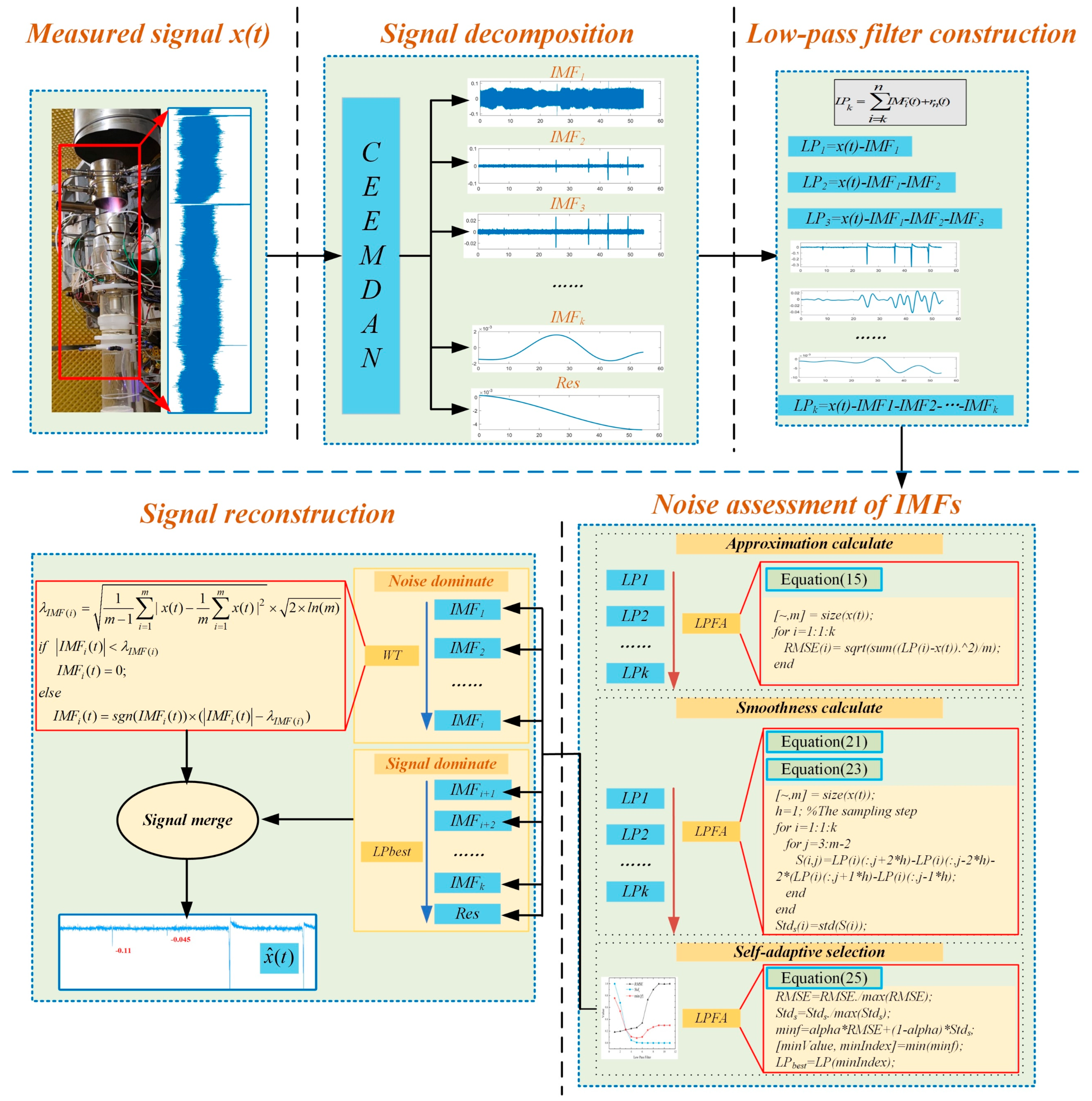
2.4. The Framework of the Proposed Method
In summary, the CEEMDAN method is used to decompose the initial electrostatic signal into multiple stationary IMF components. These components are then filtered using the proposed low-pass filtering method based on the IMFs’ adaptive optimization (LPFA) to identify the noise-containing components. Subsequently, the wavelet threshold denoising method is applied to process the remaining IMF components further. Finally, the IMF reconstruction operations are performed to achieve noise reduction of electrostatic signals. Figure 1 displays the flow chart of the whole algorithm.
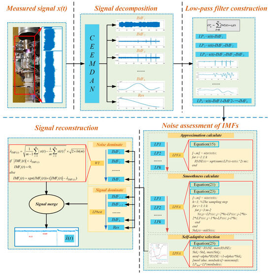
Figure 1.
The flow of the proposed noise reduction algorithm.
3. Simulation and Comparison
3.1. The Design of the Simulation Signal
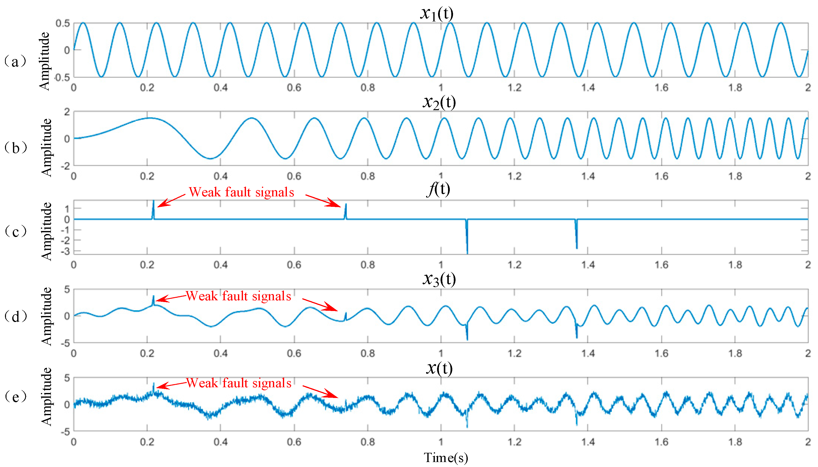
A non-stationary simulation signal that includes intermittent signals was created to assess the efficacy of the method presented in this paper. This signal was built based on the features of electrostatic signals associated with failures in aero-engine gas-path [11,16].
where x1(t) is a signal with a fixed frequency, x2(t) is a signal with a varied frequency, x3(t) is referred to as a pure electrostatic signal, x(t) is an electrostatic signal with noise, f(t) is a triangular pulse signal that simulates a fault of block dropping, n(t) is a Gaussian noise, and t is the sampling time.
The t was set to 2 s, and the sampling rate was set to 2000 Hz. Setting the 2 s sampling duration ensured we captured enough data points for reliable signal analysis while keeping the data size manageable. This duration is sufficient to observe transient behaviors in the system under study without unnecessary data redundancy. We selected a 2000 Hz sampling rate based on best practices from several studies and similar research in signal processing [19,32,33,34]. According to the Nyquist theorem, these studies recommend a sampling rate of at least twice the highest frequency component in the signal. Our experimental setup shows that the significant frequency components in the signal are well below 1000 Hz, so a 2000 Hz sampling rate ensures accurate signal reconstruction without aliasing.
The mathematical expression of the f(t) is
where t0 is the start time of the pulse, and it is set to a random value; the height of the pulse, denoted as h, is set to a random value; and T, the width of the pulse, is set to 0.005 s based on the approximate time taken for the fault particle cluster to pass through the sensor’s sensitivity area in the aero-engine fault simulation experiment described in Section 4.
It contains two positive and two negative triangular pulse signals, which can simulate the inductive signals of the dropped particles with different amounts and properties of the charged energy. When the signal-to-noise ratios (SNR) of the Gaussian noise is set to 10, the signals of x1(t), x2(t), f(t), x3(t), x(t) are shown in Figure 2, respectively.
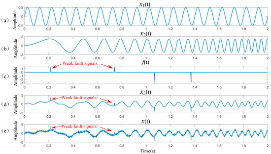
Figure 2.
The simulated electrostatic signal.
The critical parameters utilized in the subsequent analyses are as follows: the wavelet threshold is set up for a five-layer decomposition, employing the sym8 wavelet as the basis function; the influence factor α for the filter approximation is set to 0.3; the magnitude of the additional noise in CEEMDAN is set to 0.2; and the number of realizations used for averaging is set to 100. According to [25,35], adding more noise improves CEEMDAN performance, but this requires more implementations. It has been found optimal when the standard deviation of the algorithm noise is 0.2. Consequently, researchers typically use 0.2 as the level of added noise when using CEEMDAN [18]. Therefore, in this paper, the level of the added noise in CEEMDAN was also set to 0.2. The reasons for selecting the other three parameters will be discussed in detail in Section 3.3.4.
3.2. Evaluation Indicators
The denoising effect of simulated signals is commonly assessed using three widely used indicators: the signal-to-noise ratio (SNR) [28], the mean square error (MSE), and the normalized correlation coefficient (NCC) [24]. These indicators are defined as follows:
where x(t) is the original signal without noise, and is the signal after denoising. The three indicators are employed in this paper to assess the denoising effect of the algorithms.
3.3. Analysis and Discussion
3.3.1. EMD and CEEMDAN Decomposition
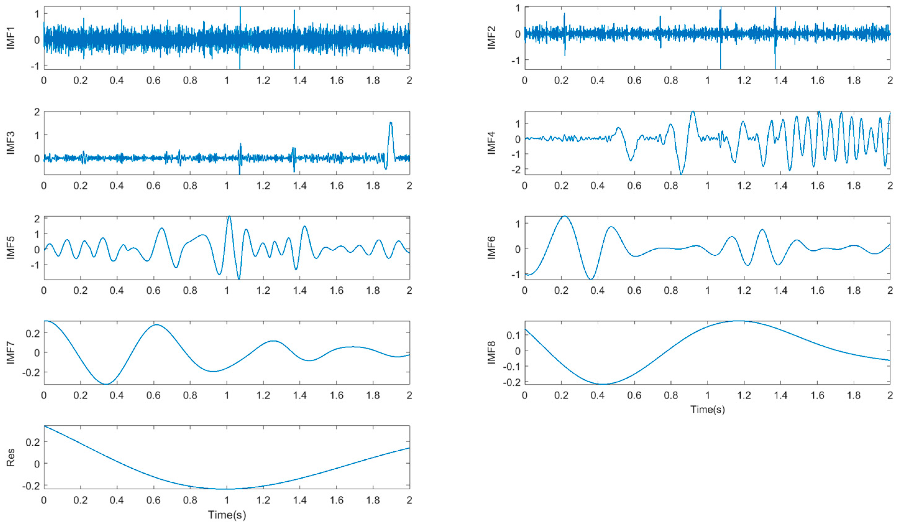
The simulation signal x(t) is decomposed according to EMD and CEEMDAN, respectively. The decomposition results are shown in Figure 3 and Figure 4. Here, the SNR of the Gaussian noise, which added up to x3(t), is set to 10. The effectiveness of signal decomposition can be observed in Figure 3 and Figure 4 for both approaches. Figure 3 demonstrates that in the case of EMD, there is a prominent trend of mixing modes in the IMFs. In Figure 4, CEEMDAN exhibits a notable enhancement in mitigating mode mixing compared to EMD. In brief, the IMF extraction method using CEEMDAN has a relatively minimal loss of precision.
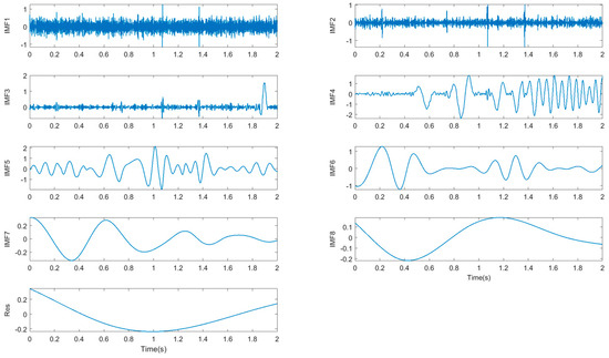
Figure 3.
The EMD results of the simulation signal x(t).
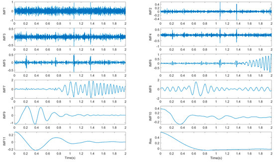
Figure 4.
The CEEMDAN results of the simulation signal x(t).
3.3.2. Analysis of IMF Selection
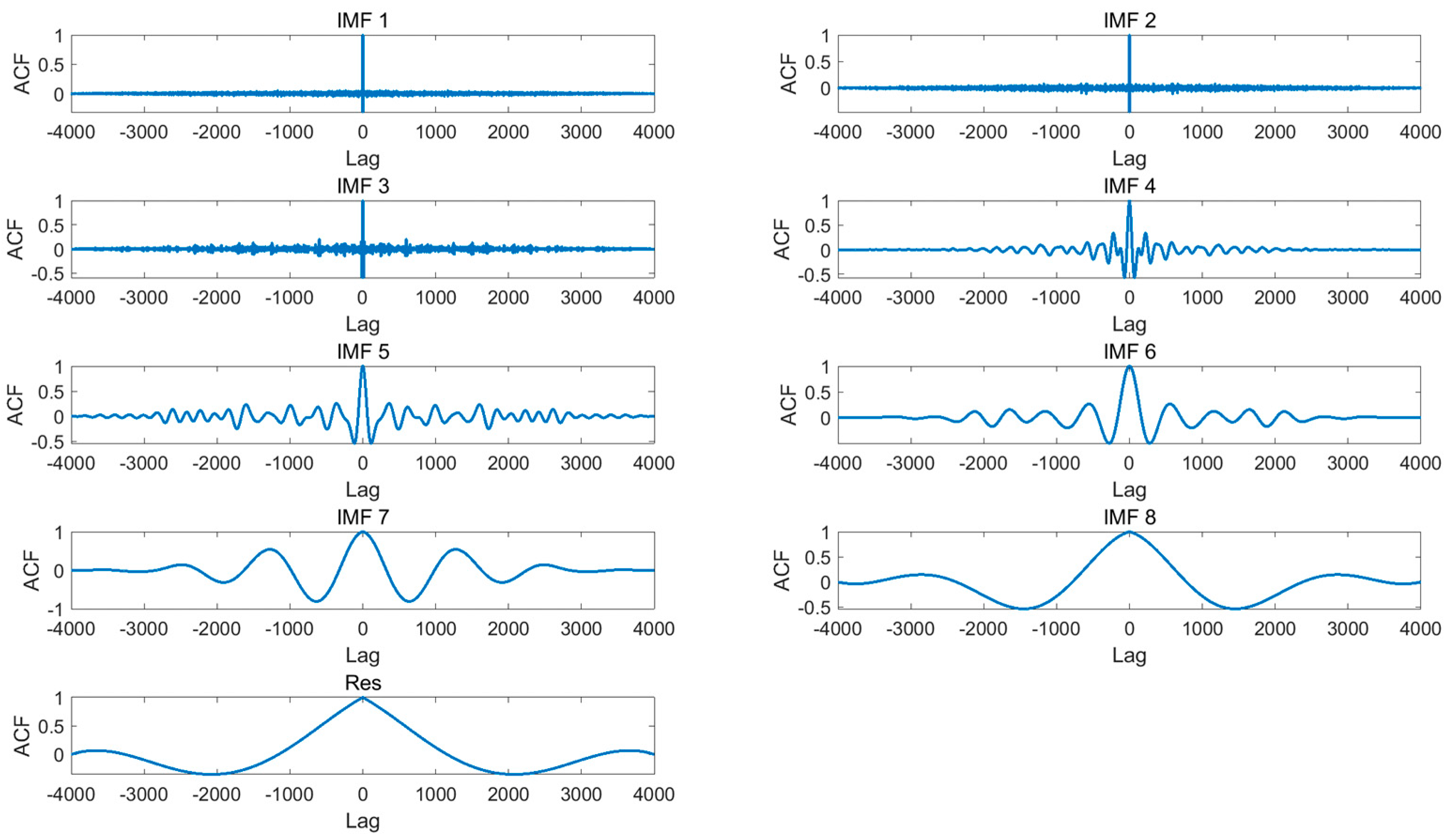
After the IMFs produced by signal decomposition have been acquired, it becomes crucial to identify between useful signals and noise signals. It is also essential for effectively employing the modal decomposition method to reconstruct signals. Neither EMD nor CEEMDAN can accurately represent all deconstructed IMFs that capture the essential characteristics of the signal x(t). The key to information extraction and interference reduction lies in the efficient extraction of IMFs. In theory, a stronger correlation between the IMFs and signal x(t) would result in a greater effectiveness of the components of x(t). It is common knowledge that the autocorrelation functions (ACF) obtained from samples are typically employed to assess the significance of the IMFs. Therefore, we use the ACFs to compare with the proposed LPFA for IMF selection.
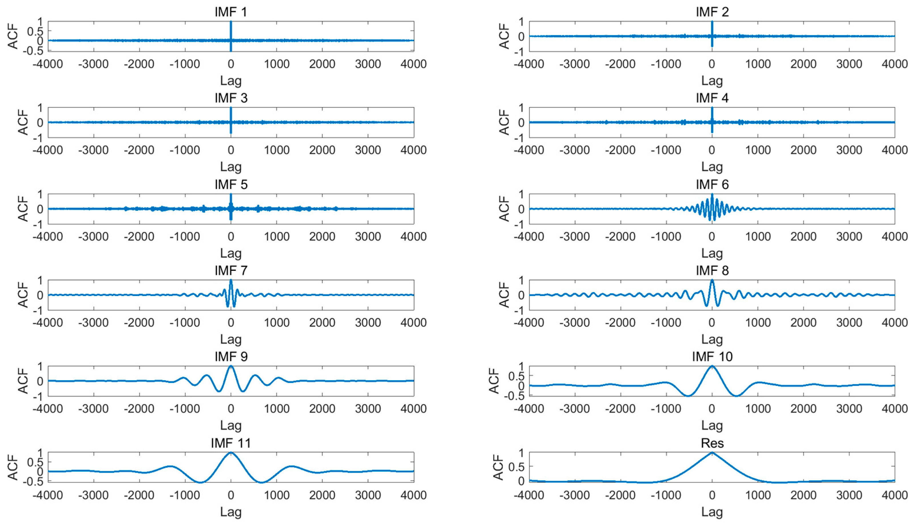
Since random noise has a weak temporal correlation, its ACF curve is usually close to the shock function. Specifically, the function achieves its highest value at the zero point, and then it rapidly diminishes to zero on both sides of the point. It is generally considered that the IMFs with such characteristics are the noise-dominated IMF components. Firstly, the electrostatic signal was decomposed using the EMD. Then, the ACF was computed for each IMF component. We can see from Figure 5 that IMF1 and IMF2 are primarily affected by noise. Therefore, the remaining IMFs were manually chosen as the signal-dominant components for the first signal reconstruction. Meanwhile, the ACF of the IMF components decomposed using the CEEMDAN, which is shown in Figure 6. It is obvious that IMF1, IMF2, and IMF3 are noise-dominated components. Therefore, the remaining IMFs were chosen as the signal-dominant components.
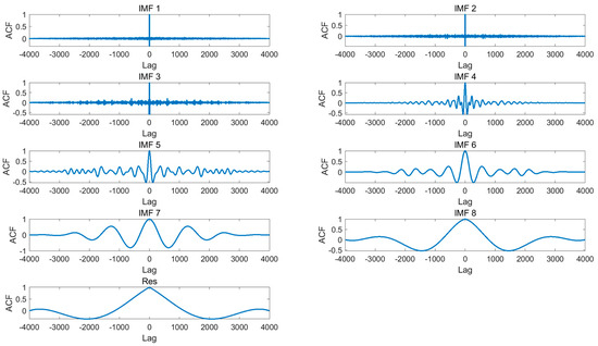
Figure 5.
The ACF of IMF components decomposed by EMD.
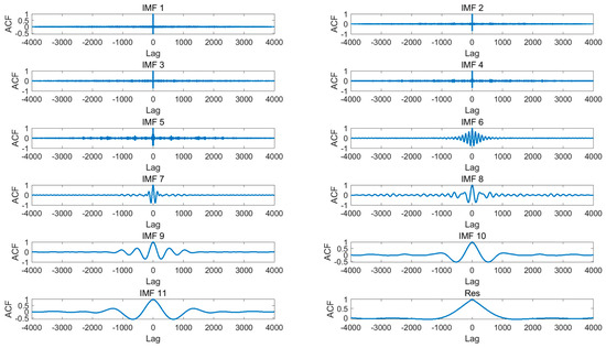
Figure 6.
The ACF of IMFs components decomposed by CEEMDAN.
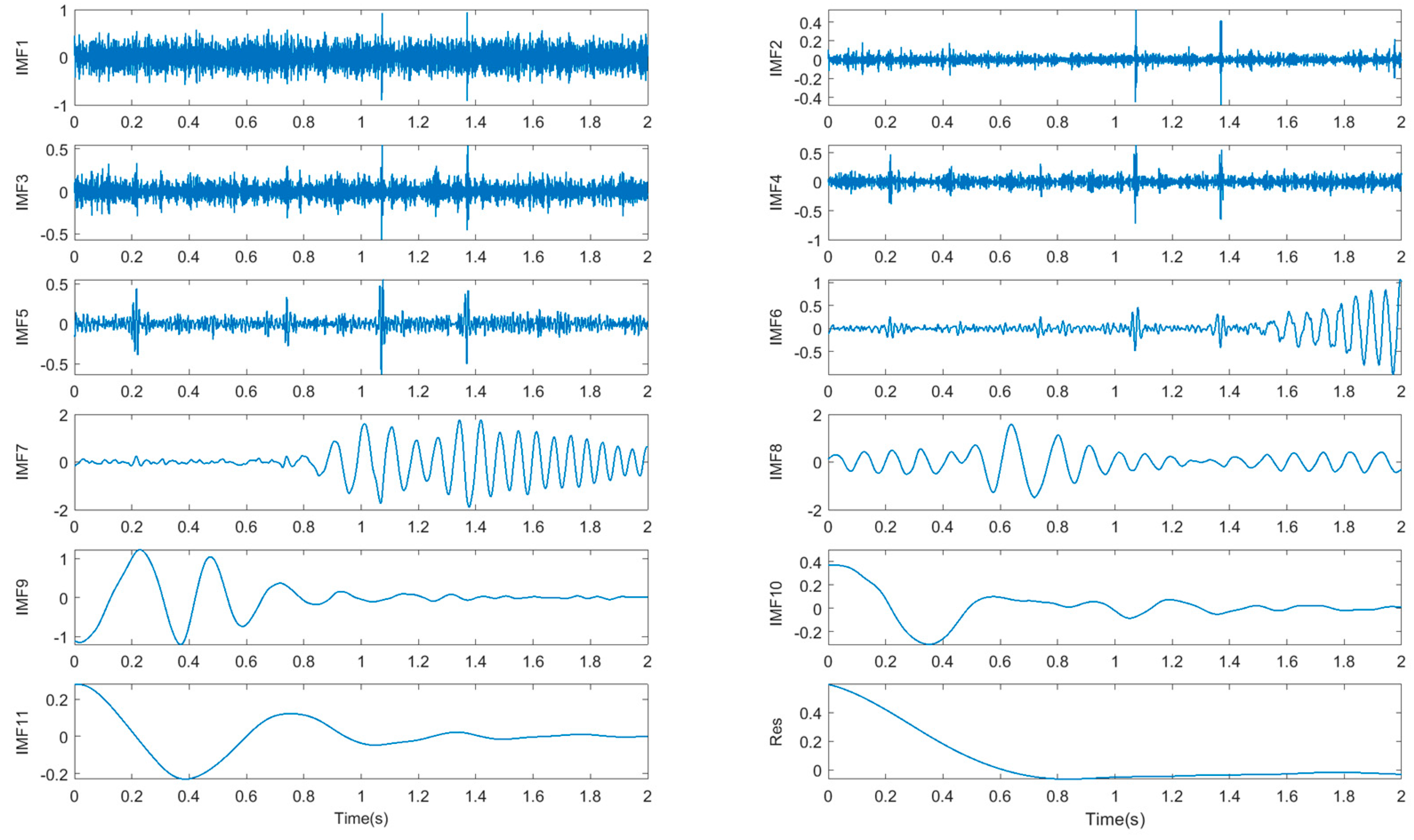
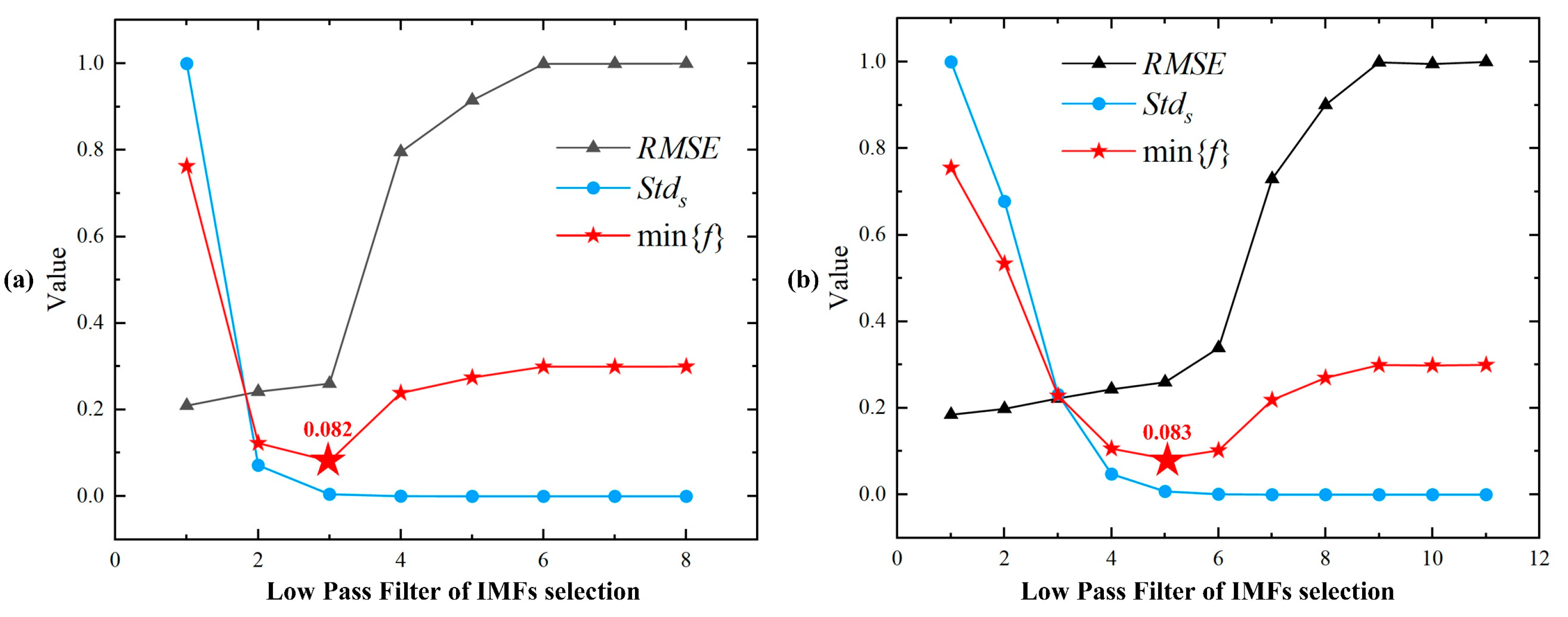
Figure 7 demonstrates the automatic selection of IMF components using LPFA. Specifically, Figure 7a depicts the process of automatic signal selection for 8 IMFs produced by EMD, and we can see that the optimal value of min{f} is 0.082, and the components automatically selected by LPFA are IMF4-IMF8. Figure 7b illustrates the process of automatic signal selection for 11 IMFs produced by CEEMDAN, and we can see that the optimal value of min{f} is 0.083, and the components automatically selected by LPFA are IMF6-IMF11.
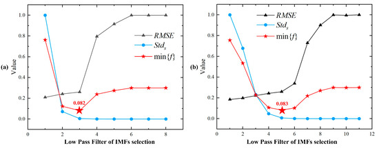
Figure 7.
The selection of IMFs by the LPFA: (a) EMD; (b) CEEMDAN.
3.3.3. Useful Information Re-Extracted by WT
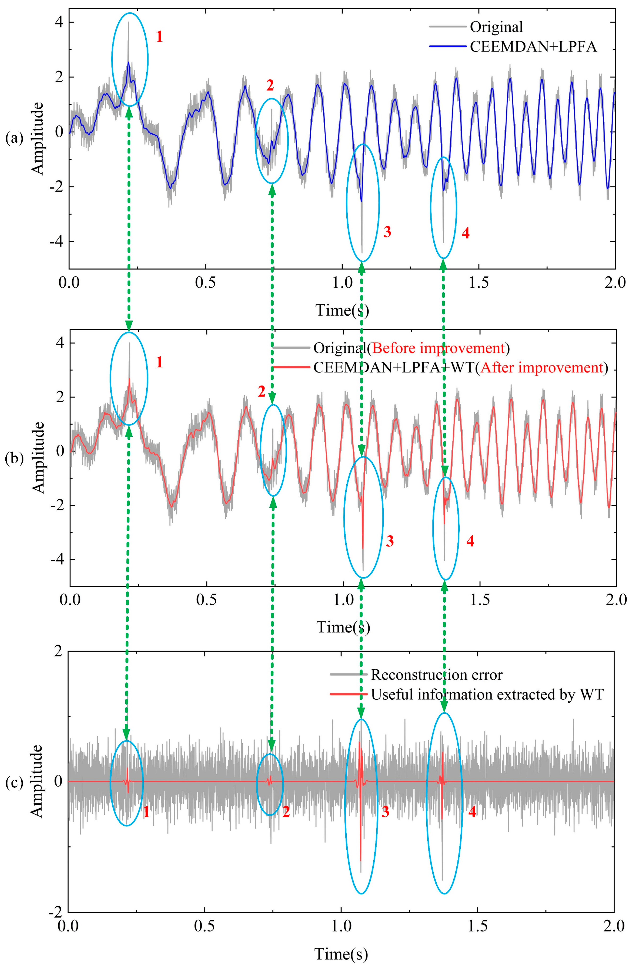
Following the selection of the IMF components in the previous step, the signal reconstruction operation was promptly performed. However, a significant problem came out. That is, the unselected IMF components still retained valuable information. Figure 8a compares the signal after CEEMDAN + LPFA reconstruction and the original signal, while Figure 8b illustrates the comparison between the signal after CEEMDAN + LPFA + WT (the proposed method) reconstruction and the original signal. Figure 8c shows the error of the signal after CEEMDAN + LPFA reconstruction and useful information extracted by WT. The WT method extracts much useful information again in the local elliptic region of the reconstructed error signal. The original signal’s third and fourth faults cannot be successfully extracted without using the WT. However, the information on these two faults is effectively extracted after employing the WT. This is extremely important for the diagnosis of block drop-type faults in aero-engine gas paths.
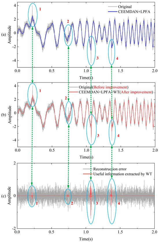
Figure 8.
(a) Reconstructed signal by CEEMDAN + LPFA; (b) reconstructed signal by CEEMDAN + LPFA + WT; (c) reconstruction errors by CEEMDAN + LPFA and useful information extracted by WT.
3.3.4. The Results of Denoising Performance with Different Parameters
In Section 3.1, we chose wavelet function sym8, the influence factor 0.3, and the realization number 100 in this paper. Generally, parameters often affect the noise reduction performance. Therefore, different parameters of the proposed method were investigated on the simulation signal. Three factors in particular, including wavelet function, influence factor of filter approximation, and realization number, need to be determined.
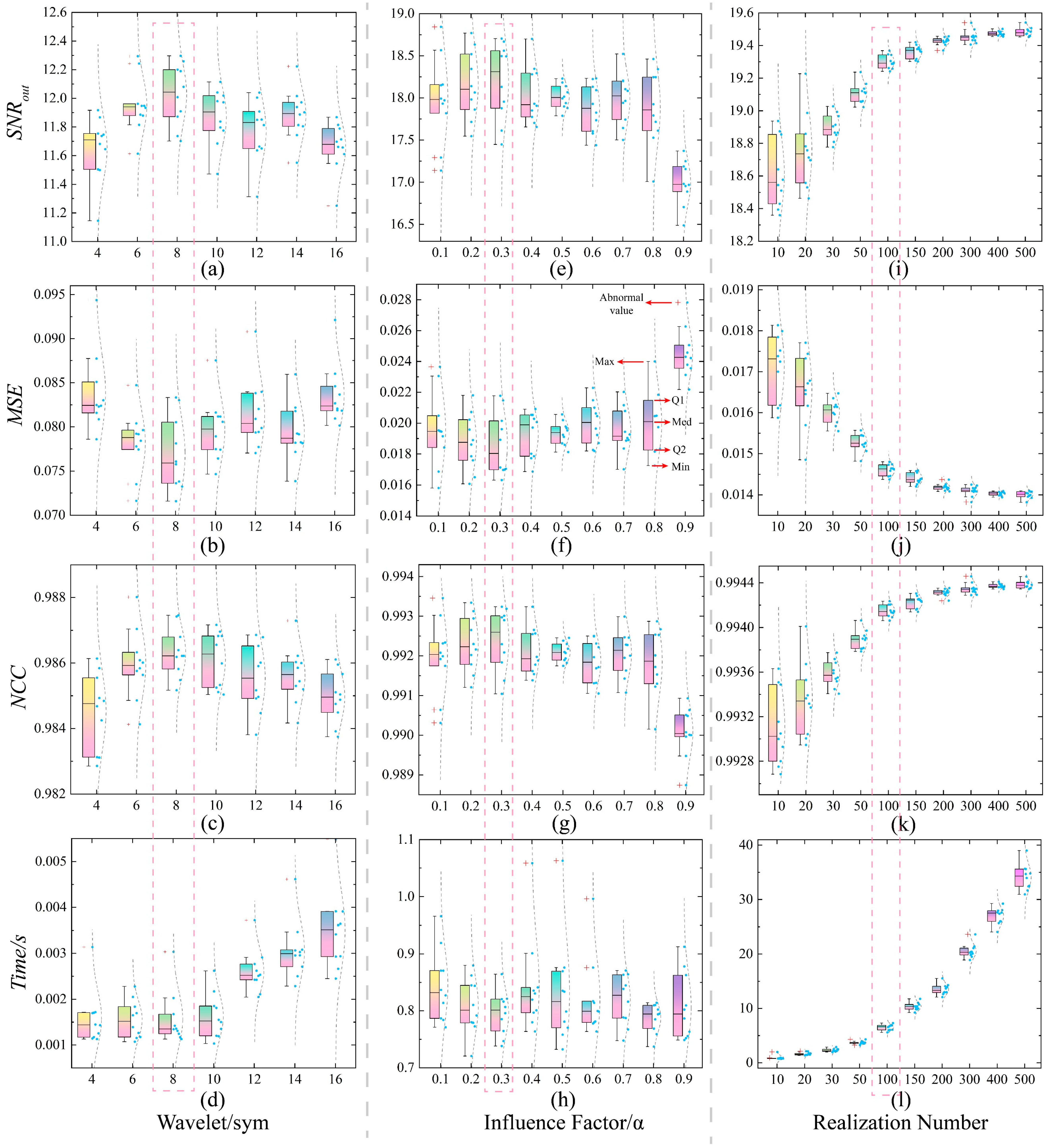
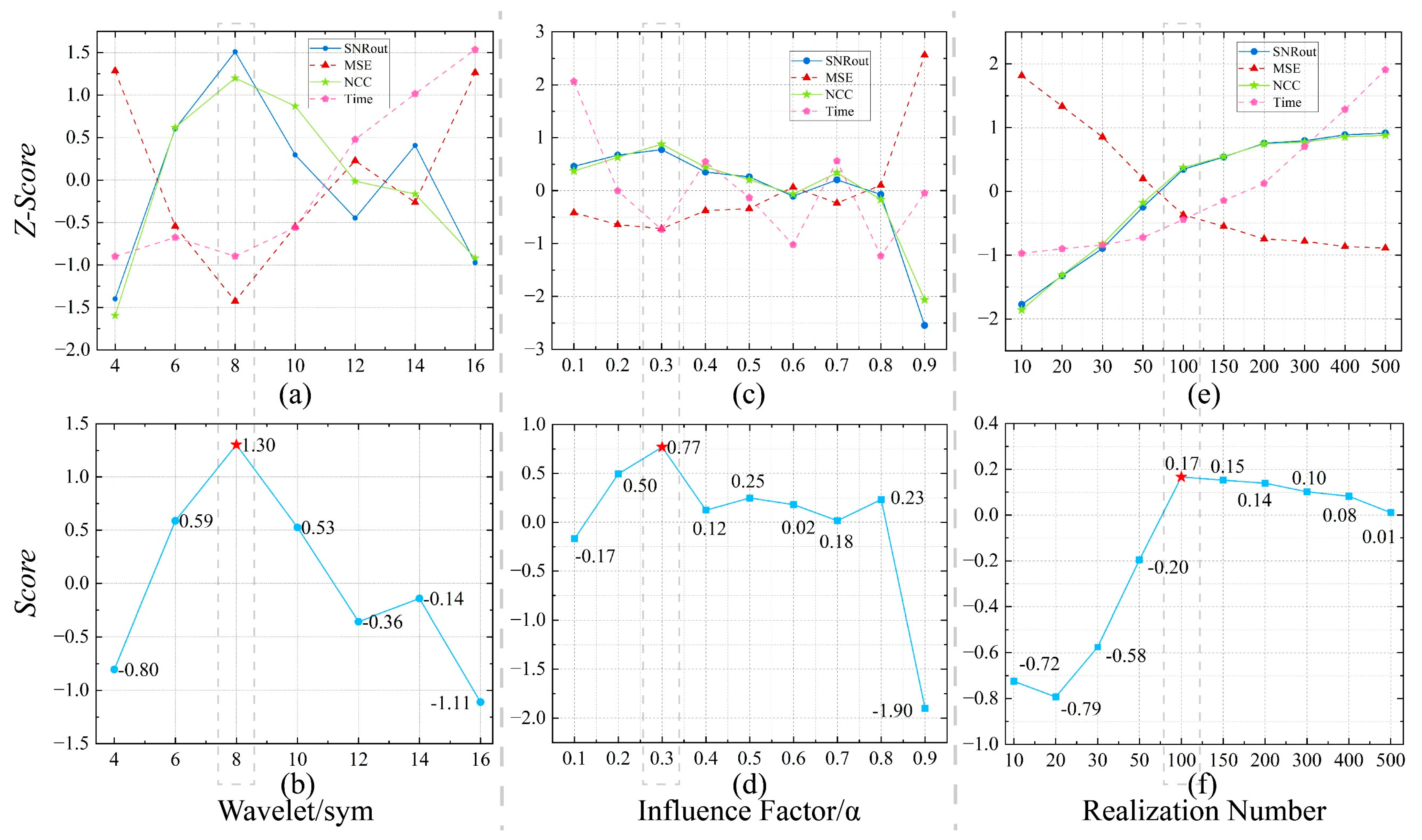
To fully account for the impact of these factors, Figure 9a–l present the SNRout, MSE, NCC, and Time values of signal denoising over 10 times in experiments. The box plots contain five numerical points: a maximum value (Max), a minimum value (Min), an upper quartile (Q1), a lower quartile (Q2), and a median (Med). The box plot describes the relatively stable tendency of the data without the influence of abnormal values.
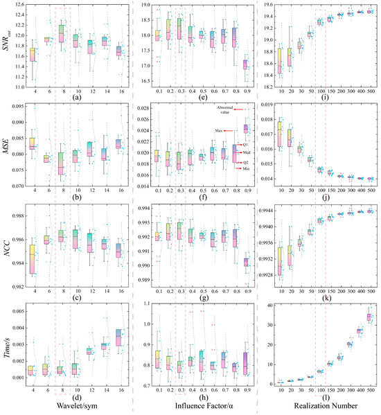
Figure 9.
The results of denoising performance with different parameters. (a–d) Box plots of SNRout, MSE, NCC, and Time values in different wavelet functions. (e–h) Box plots of SNRout, MSE, NCC, and Time values in different influence factors. (i–l) Box plots of SNRout, MSE, NCC, and Time values in different realization numbers.
To more clearly describe the trends in noise reduction performance of SNRout, MSE, NCC, and Time values under different parameters, the Z-Score normalization method [36] was used to standardize the range of all variables.
where x represents the Root Mean Square (RMS) of the SNRout, MSE, NCC, and Time values from 10 experiments; Z-Score(x) represents the standardization data; and μ and σ denote the mean and standard deviation of x, respectively. Normalization helps to ensure that all variables associated with all operating conditions are considered equally.
When comparing the performance of the four parameters, SNRout, MSE, NCC, and Time, larger values of SNRout and NCC are better, while smaller values of MSE and Time are preferred; we introduced a Score value to unify the comparison scale of these parameters. The Score value is calculated using the following formula:
where x represents the Root Mean Square (RMS) of the SNRout, MSE, NCC, and Time values from 10 experiments; Z-Score (SNRout) represents the standardization data of SNRout values; Z-Score (NCC) represents the standardization data of NCC values; Z-Score (MSEre) represents the standardization data of MSEre values; Z-Score (Timere) represents the standardization data of Timere values; and Score represents the overall performance of the four parameters SNRout, MSE, NCC, and Time.
A larger Score value indicates better noise reduction effectiveness of the signal, while a smaller Score value indicates poorer noise reduction effectiveness.
Figure 10a–f show the Z-Score values and Score values of all performance indicators. They summarize the impact of the parameters on the noise reduction performance.
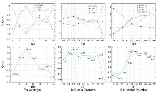
Figure 10.
The normalized comparison of denoising performance. (a,b) Z-Score and Score values in different wavelet functions. (c,d) Z-Score and Score values in different influence factors. (e,f) Z-Score and Score values in different realization numbers.
- (1)
- Effects of the wavelet function
In the WT method, the multi-scale decomposition capability of the wavelet transform is utilized to separate noise from useful information in the signal. Among these, the wavelet function plays a core role, as its selection directly affects the decomposition effectiveness. The box plots of the SNRout, MSE, NCC, and Time values for the signal noise reduction in different sym wavelet functions are presented in Figure 9a–d.
It can be observed that the results corresponding to different wavelet functions show significant differences. The noise reduction performance improves gradually from sym4 to sym8 but shows a slow declining trend from sym8 to sym16. Additionally, from sym4 to sym10, the algorithm processing time is similar, but starting from sym12, there is a noticeable increase in processing time. This indicates that although the processing time of the algorithm increases with the number of wavelet decomposition levels, the noise reduction performance does not continue to improve.
Figure 10a shows the normalized comparison of the four noise reduction evaluation indicators, SNRout, MSE, NCC, and Time, under different wavelet functions. It can be clearly seen that when using the sym8 wavelet function, the values of SNRout and NCC are the highest, while the values of MSE and Time are the lowest. This indicates that the noise reduction effect is optimal when using sym8, as also demonstrated by Figure 10b. Therefore, in this paper, the wavelet function was set to sym8.
- (2)
- Effects of the influence factor
As discussed in Section 2.2.2, we know that the influence factor α balances signal fluctuation and smoothness. For noise reduction of the simulated signal, the influence factor α is set to be between 0.1 and 0.9. Figure 9e–h show the noise reduction results. It can be observed that as α increases from 0.1 to 0.3, SNRout and NCC gradually increase, while MSE gradually decreases. From 0.3 to 0.9, SNRout and NCC gradually decrease, and MSE gradually increases, indicating that the noise reduction performance first improves and then declines. Regarding processing time, the algorithm’s processing time remains similar for different values of α, with no significant differences.
Figure 10c shows the normalized comparison of the four noise reduction evaluation indicators, SNRout, MSE, NCC, and Time, under different influence factors α. When α = 0.3, SNRout and NCC are at their highest values, MSE is at its lowest value, and Time is relatively moderate. Conversely, when α = 0.9, the noise reduction performance is the worst. Figure 10d shows the overall Score of noise reduction performance under different influence factors. This Score indicates that the noise reduction effect is optimal when α = 0.3. Taking the evaluation criterion into account, the influence factor is set to 0.3.
- (3)
- Effects of the realization number
The realization number in the CEEMDAN method represents the number of independent noise additions performed to enhance algorithm stability and reduce mode mixing. By repeating this process multiple times and averaging the results, more stable and accurate signal decomposition results can be obtained. The typical value for the number of realizations is chosen between 20 and 500 [18,25,28]. To more comprehensively verify the noise reduction capability corresponding to different realization numbers, the realization number is set to be 10, 20, 30, 50, 100, 150, 200, 300, 400, and 500.
As shown in Figure 9i–l, it can be clearly seen that, generally, a larger realization number leads to better performance with respect to SNRout, MSE, and NCC, indicating that a larger realization number can enhance the signal noise reduction effect. However, from the perspective of time consumption, the larger the realization number, the longer the algorithm processing time. The aim of signal processing is to minimize time consumption while achieving excellent noise reduction performance. From Figure 9i–k, we find that when the realization number is 100, the noise reduction performance is already sufficiently excellent. Beyond this point, increasing the realization number further results in a gradual improvement in noise reduction performance but a rapid increase in time consumption.
From Figure 10e, we see that when the realization number is 100, the balance of all performance indicators is relatively ideal. Figure 10f also shows that the Score value is optimal at this realization number. Considering both noise reduction performance and time consumption, the realization number is set to be 100.
3.3.5. Effect of Ablation Experiment on Denoising Performance
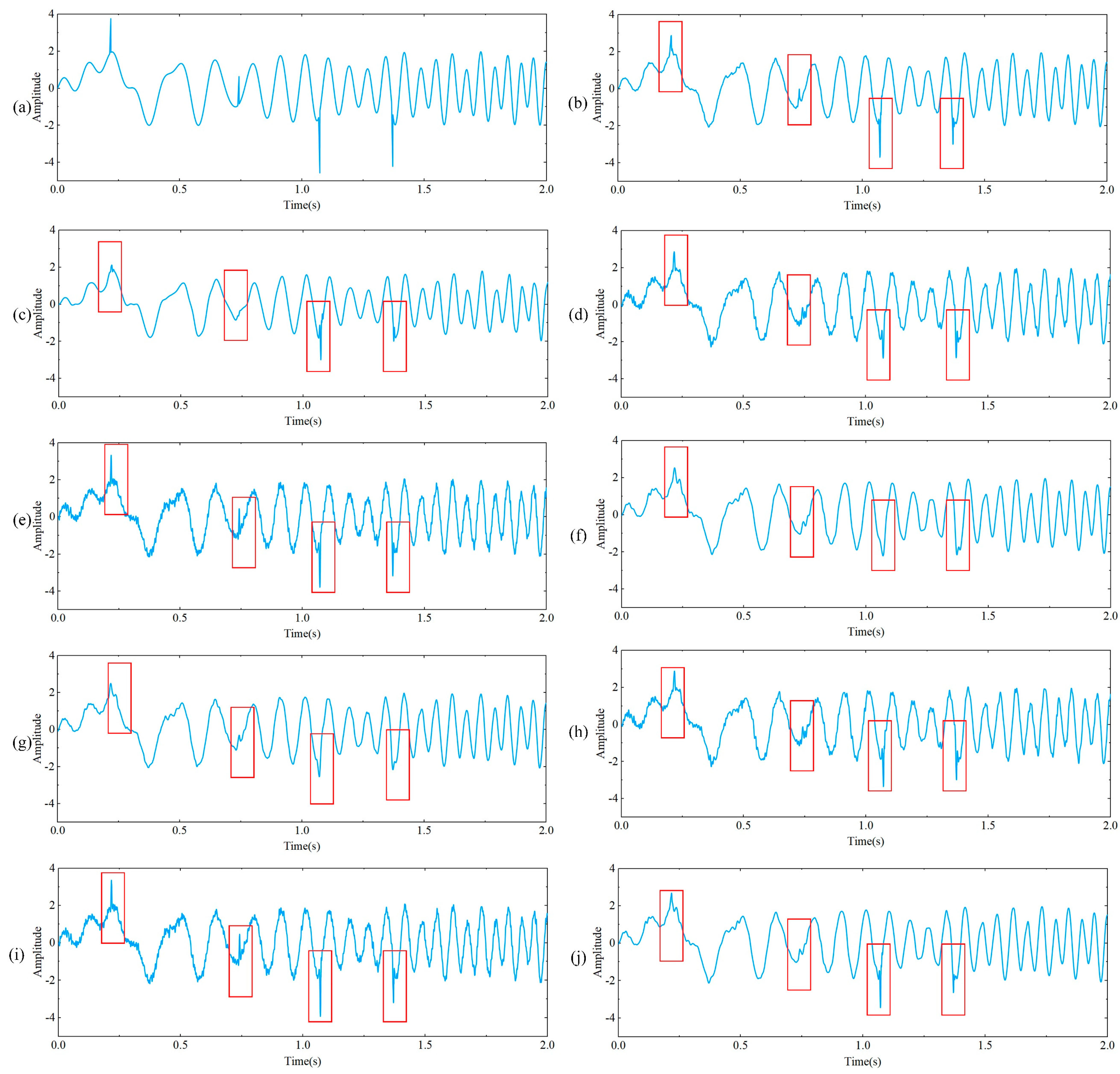
EMD, ACFs, and WT are extensively applied signal processing methods [13,14,15,24,37] which have been demonstrated to possess a strong denoising capability for machinery faults. Therefore, an ablation experiment is conducted to explore the contribution of alternative strategies to the improvement in performance. Figure 11 shows a total of eight different combination approaches being evaluated for comparison, including WT, EMD + ACF, CEEMDAN + ACF, EMD + LPFA, CEEMDAN + LPFA, EMD + ACF + WT, CEEMDAN + ACF + WT, and EMD + LPFA + WT.
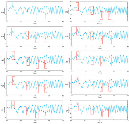
Figure 11.
Simulated denoising signal comparisons: (a) pure original signal; (b) the proposed method; (c) WT; (d) EMD + ACF; (e) CEEMDAN + ACF; (f) EMD + LPFA; (g) CEEMDAN + LPFA; (h) EMD + ACF + WT; (i) CEEMDAN + ACF + WT; (j) EMD + LPFA + WT.
Figure 11a displays the original signal (pure signal), and Figure 11b shows the denoised result obtained using the proposed method. The denoising signal exhibits a high level of consistency with the pure signal, which indicates the excellent performance of the proposed denoising method. Figure 11c–j displays the denoising signal comparisons, where the WT, EMD + LPFA, and CEEMDAN + LPFA denoising methods fail to reconstruct the weak fault signals. We can also see that the local structure in the rectangular of the other five methods is less excellent than that of the proposed method. The proposed method has a more vital ability to extract the weak fault signals and is the most similar waveform to the pure signal.
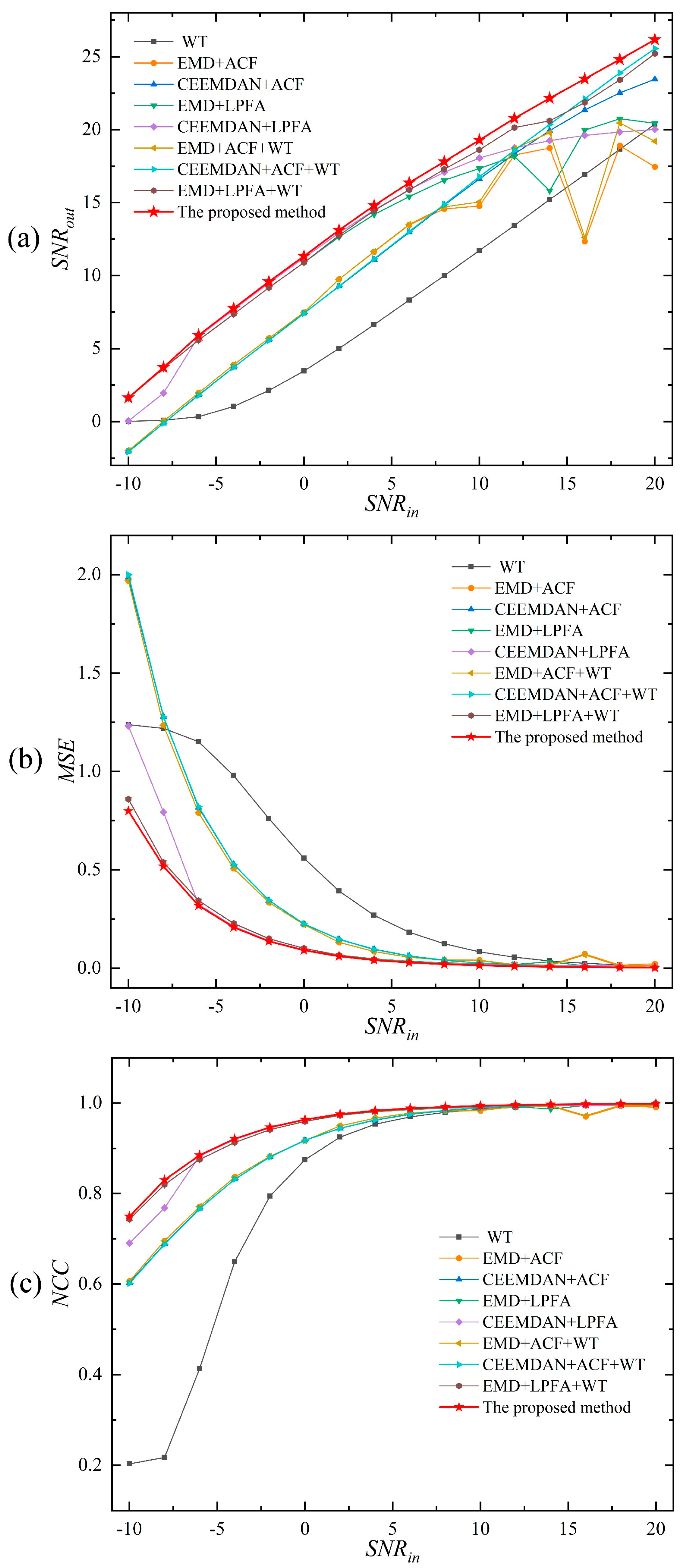
Because the clean signal is known in advance, the output signal-to-noise ratio (SNRout), MSE, and NCC are also applied to evaluate the denoising performance, as shown in Figure 12. It is observed that the proposed method achieves a higher SNRout and NCC than other methods overall. It also has a lower MSE than other methods simultaneously, indicating that the proposed method has a better denoising ability and robustness.
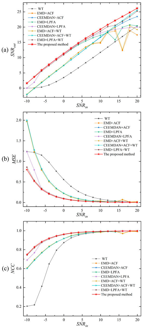
Figure 12.
Comparisons with different SNRin.
3.3.6. Denoising Performance Comparisons with State-of-the-Art Methods
To verify the effectiveness and superiority of the proposed method, some state-of-the-art methods in recent years have been used for comparison. Table 1 illustrates the signal noise reduction results for the simulation signals discussed in Section 3.1.

Table 1.
Comparisons between different methods.
In Table 1, we present a comparison of our proposed method against five contemporary approaches for electrostatic signal denoising: EMD-IMF1-IMF2-IMF3, EMD + Energy Values Select, VMD + Kurtosis + Permutation Entropy, TVD, and EMD + ACF.
- (1)
- The EMD-IMF1-IMF2-IMF3 method (after EMD, the first three IMF components are removed, and the remaining IMF components are reconstructed to form the denoised signal) presented in a 2024 study, demonstrated relatively excellent denoising performance, with an output SNRout of 17.134 dB, an MSE of 0.024, and a NCC of 0.990. This method achieved automatic processing by effectively selecting IMF components to reduce noise, although it still has limitations under extreme noise conditions.
- (2)
- The EMD + Energy Highest Values method, proposed in 2023, showed significantly poorer denoising performance, with an SNRout of only 1.775 dB, an MSE of 0.825, and an NCC of 0.579. This method automatically selects the IMF with the highest energy value for signal reconstruction, but the high-energy IMF may still contain considerable noise components, leading to poor denoising results.
- (3)
- In a 2023 study, the VMD + Kurtosis + Permutation Entropy method achieved an SNRout of 3.085 dB, an MSE of 0.610, and an NCC of 0.721 by manually specifying the number of VMD modes. This method employs VMD and IMF selection based on kurtosis and permutation entropy for denoising. However, the requirement to manually specify the number of decomposition modes adds complexity and may lead to inconsistent results under varying signal conditions.
- (4)
- The TVD method, introduced in 2022, demonstrated solid denoising performance with an SNRout of 10.987 dB, an MSE of 0.099, and an NCC of 0.962. This method uses TVD to effectively reduce noise while preserving the main features of the signal, achieving automatic processing.
- (5)
- The EMD + ACF method, proposed in 2021, combines EMD with autocorrelation function selection, achieving better denoising performance with an SNRout of 15.853 dB, an MSE of 0.032, and an NCC of 0.987. Despite its good performance, the need for manual ACF selection increases the complexity of the process.
- (6)
- The proposed method in this study significantly outperformed the other methods in terms of denoising performance, achieving an SNRout of 19.319 dB, an MSE of 0.014, and an NCC of 0.994. By utilizing optimized signal decomposition and re-extracting useful information techniques, our method maximally reduces noise components while preserving the main features of the signal, demonstrating superior denoising capability and application potential with automatic processing.
The comparative analysis shows that the proposed denoising method outperforms existing methods in all performance metrics, particularly in maintaining signal quality and suppressing noise. The realization of automatic processing further enhances the method’s practicality, providing a new effective approach for efficient denoising of electrostatic signals.
4. Experimental Analysis
4.1. Test Environment
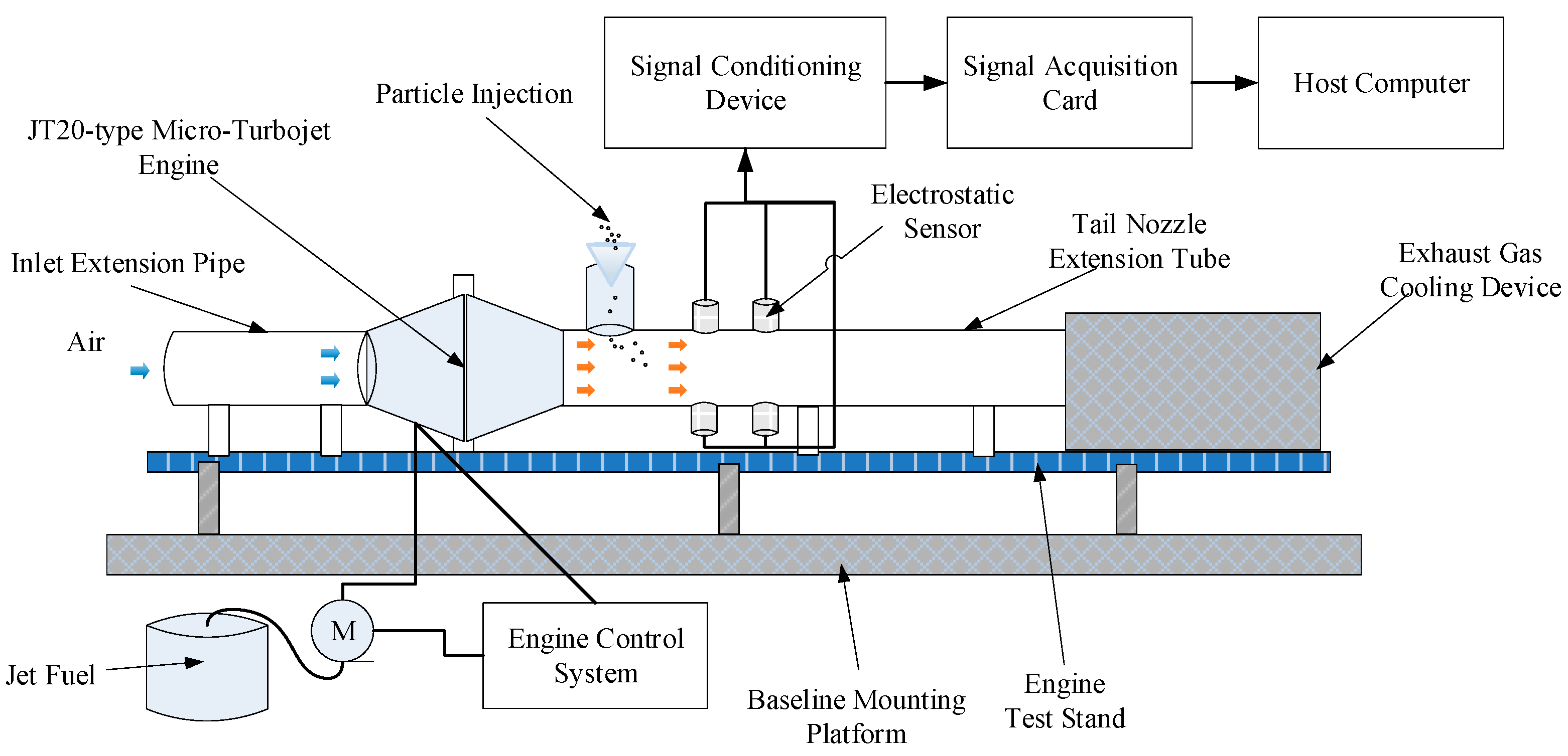
This section provides an experimental microturbine engine setup to simulate faults in a real aero-engine. The focus of electrostatic monitoring lies in studying abrasive particles generated by wear-type faults in the engine gas path. A typical indication of a falling block fault in an engine is a particle group carrying a high charge at the tail nozzle of the engine’s gas path, whose electrostatic signal is characterized by a triangular pulse [6,38]. These particle groups are crucial in reflecting specific fault characteristics of the gas path. To prove the effect of the proposed signal denoising method under actual engine conditions, a JT20-type micro-turbojet engine electrostatic monitoring test bench is established. Figure 13 provides a schematic of the experimental system.
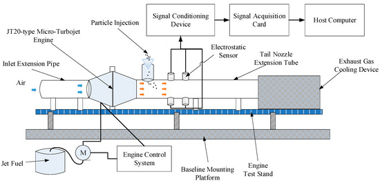
Figure 13.
The schematic of the experimental system.
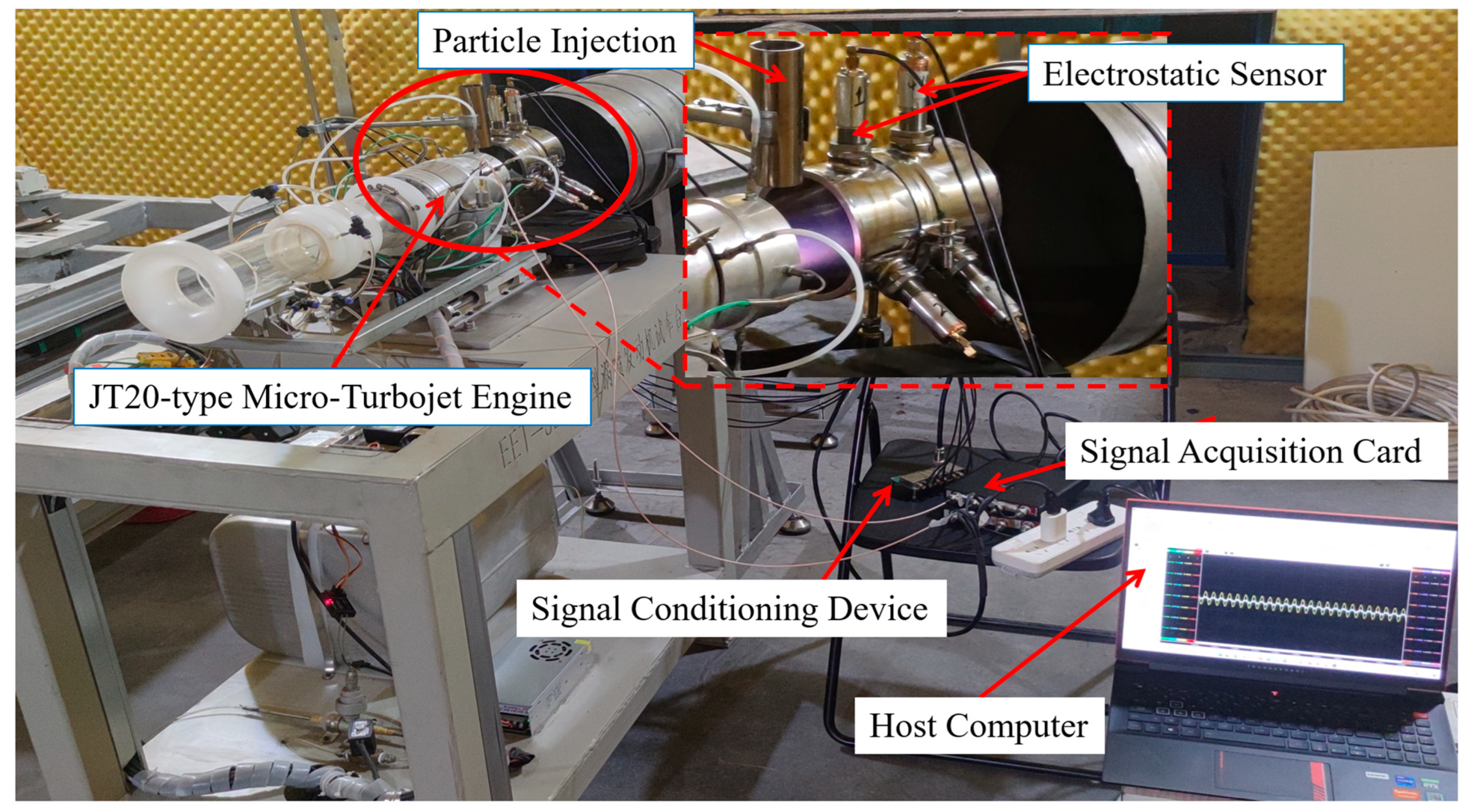
The fault simulation experiment platform system primarily comprises several components: (1) A JT20-type micro-turbojet engine (a small turbojet engine with 20 kg of thrust) and its control devices; (2) an inlet extension pipe; (3) a tail nozzle extension tube, particle injection equipment, and exhaust gas cooling device; and (4) an electrostatic signal acquisition system, including an electrostatic sensor, signal conditioning circuit, signal acquisition card, and host computer. The system’s work principle is that air sequentially passes through the components: the inlet extension pipe, the small turbojet engine, the tail nozzle extension tube, and the exhaust gas cooling device. During the experiment, the particle injection device injects the test particles into the engine’s exhaust duct. Their electrostatic levels are monitored by the custom-designed, non-invasive electrostatic sensor located inside the extension tube of the tail nozzle. The injection point was approximately 10 cm from the electrostatic sensor. Figure 14 shows a physical representation of the experimental setup.

Figure 14.
The physical representation of the experimental setup.
4.2. Data Acquisition
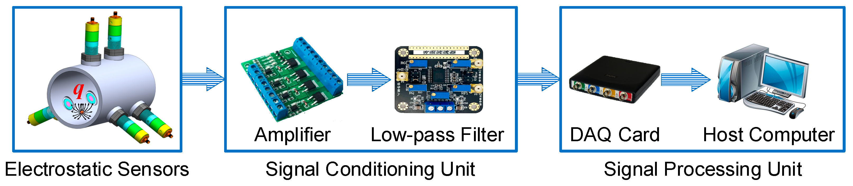
To suppress noise from the environment, the signals from the sensor electrodes were transmitted to the signal conditioning unit through coaxial cables. The electrical signals from the sensors were amplified and filtered by the signal conditioning unit. Subsequently, the signals were sampled using a data acquisition card and processed by the host computer. The block diagram of the measurement system is illustrated in Figure 15. In this experiment, the data acquisition card’s sampling rate was 2000 Hz.
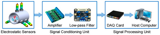
Figure 15.
Block diagram of the measurement system.
4.3. Results and Discussion
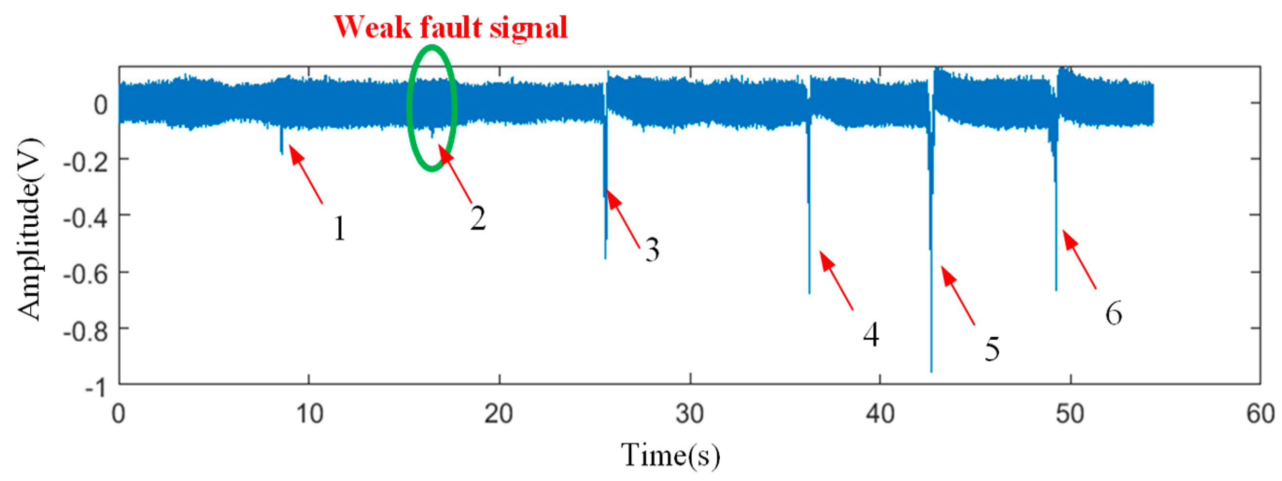
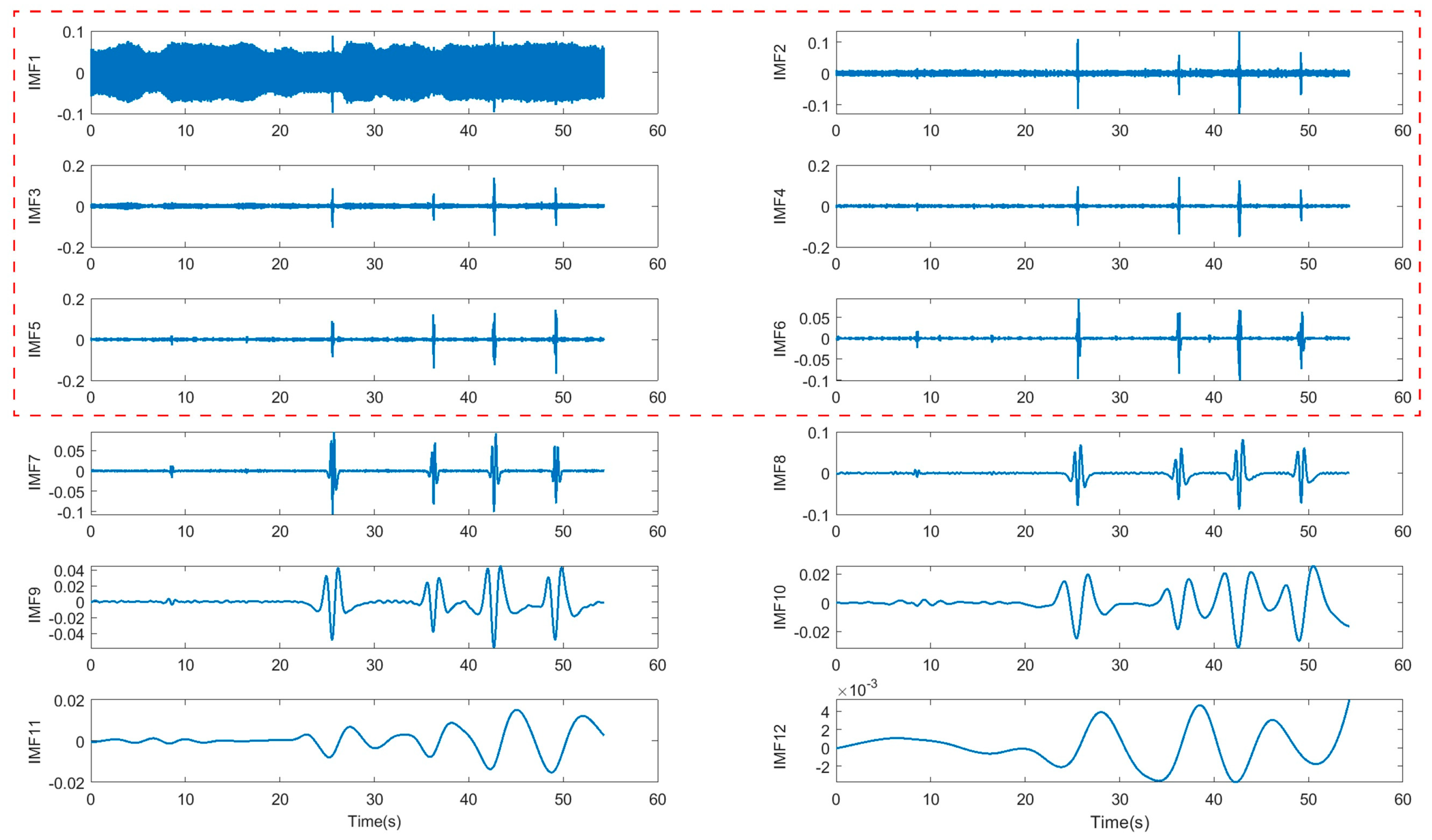
The micro-turbojet engine was injected with varying volumes of fault particles. A total of six times the faults were artificially made, as shown in Figure 16. It is evident that the original electrostatic signal contains a large amount of background noise in the working environment, making the second fault signal nearly indistinguishable from the noise. This significantly limits the precision of extracting the fault features from the electrostatic signal. The electrostatic signal was decomposed according to EMD first, and the decomposition result is shown in Figure 17. We can see that it contains 9 IMFs. The modal mixing trend of IMFs is pronounced. Then, the CEEMDAN is employed to decompose the signal, and there are 21 IMFs. Figure 18 demonstrates the first 12 IMFs of the fault signal, which has already included the primary fault information and in the proposed method used below, the first 6 IMFs are filtered out by LPFA and then undergo WT for secondary useful information extraction.
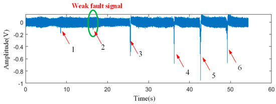
Figure 16.
Fault electrostatic signals of micro-turbojet engine.
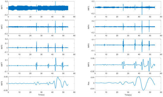
Figure 17.
Fault signal decomposed by EMD.
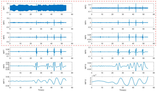
Figure 18.
The first 12 IMFs of the fault signal decomposed by CEEMDAN.
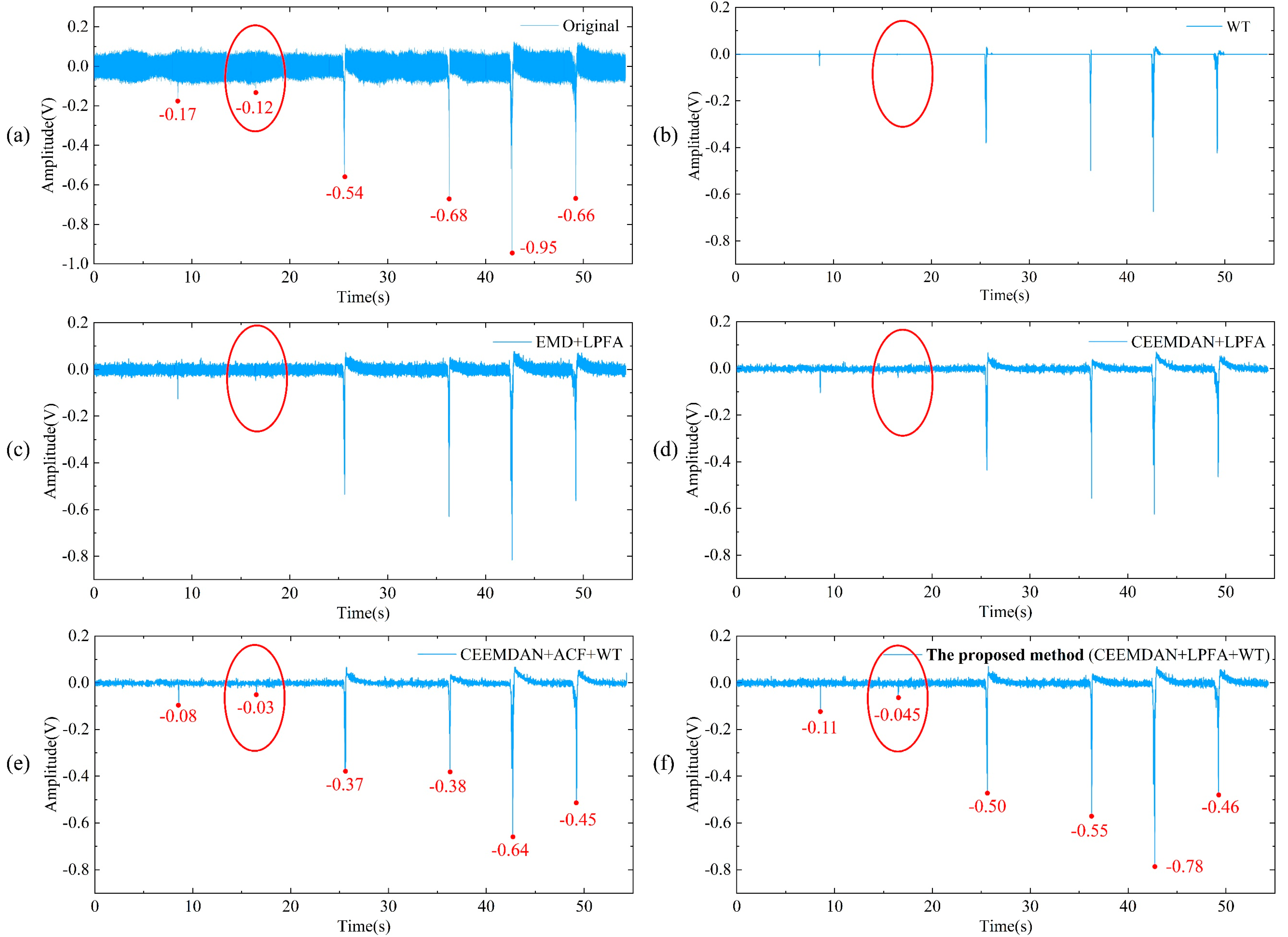
As discussed in Section 3.3.5, here, we chose five methods to compare the denoising effect of the electrostatic signal, as illustrated in Figure 19. The WT is the worst among these methods because the second fault feature was not extracted successfully. The electrostatic detail signal characterizing the normal engine operating conditions was over-filtered.
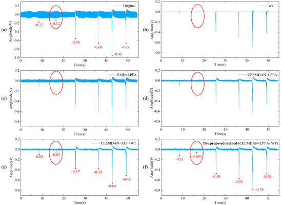
Figure 19.
Comparison of the five denoising methods: (a) original signal; (b) WT; (c) EMD + LPFA; (d) CEEMDAN + LPFA; (e) CEEMDAN + ACF + WT; (f) the proposed method (CEEMDAN + LPFA + WT).
Although the second method of EMD + LPFA in Figure 19c is slightly better than WT in electrostatic detail signal feature extraction, its background noise is more significant relative to the CEEMDAN-based denoising method. We can see in Figure 19d that the CEEMDAN + LPFA has a better denoising ability than the WT and EMD + LPFA, proving the superiority of CEEMDAN over EMD.
Figure 19e,f display the denoising effect of CEEMDAN + ACF + WT and the proposed method (CEEMDAN + LPFA + WT). Both methods exhibit outstanding performance in extracting weak fault signals compared to the previous three methods. The proposed method shows superior accuracy in extracting fault information compared to CEEMDAN + ACF + WT, as it can closely approximate the original signal amplitude. Most importantly, the ACF method primarily depends on the manual selection of IMF components for signal reconstruction, while the LPFA developed in this study exploits an algorithm that selects IMFs automatically. This automated selection procedure makes the proposed method highly suitable for deployment in real industrial applications. In addition, when comparing Figure 19d with Figure 19f, it is evident that the initial extraction of signal features using CEEMDAN + LPFA provides plenty of valuable signal features, which can be further extracted after using WT. Notably, the second fault can be distinctly illustrated.
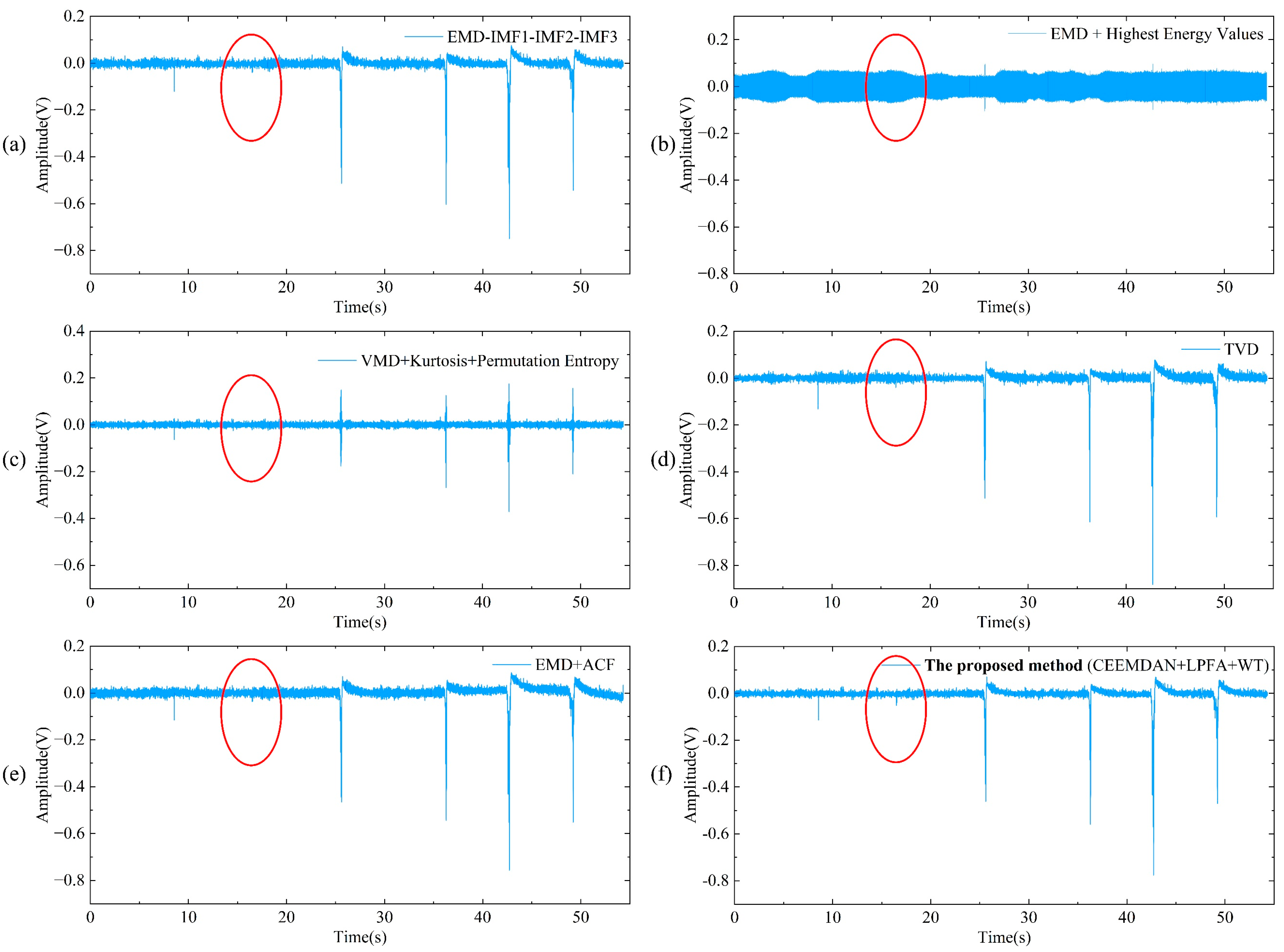
As discussed in Section 3.3.6, we compared the noise reduction performance of the proposed method with state-of-the-art methods using real measured data, as shown in Figure 20.
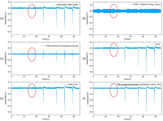
Figure 20.
Comparison of state-of-the-art methods: (a) EMD-IMF1-IMF2-IMF3; (b) EMD + Highest Energy Values; (c) VMD + Kurtosis + Permutation Entropy; (d) TVD; (e) EMD + ACF; (f) the proposed method (CEEMDAN + LPFA + WT).
- (1)
- Figure 20a shows the denoised signal obtained by deleting the first three IMF components and reconstructing the signal after EMD [14]. The plot shows that while this method effectively reduces some of the noise, there are still noticeable noise components present, particularly highlighted within the red circle, leading to the weak signal being overwhelmed. The signal retains some of the original features, but the presence of residual noise affects the overall quality of the denoising.
- (2)
- Figure 20b shows the result of the denoised signal obtained by selecting the IMF with the highest energy value after EMD [13]. The plot indicates that this approach leads to significant residual noise, making it nearly impossible to extract the fault signal. This result suggests that selecting only the highest energy IMF may not be sufficient for effective noise reduction, as the high-energy components can still contain substantial noise.
- (3)
- Figure 20c shows the denoising result using the VMD + Kurtosis + Permutation Entropy method [17]. This method can extract some fault signals, but as indicated by the red circle, it also fails to effectively extract weak fault signals. The value of the first fault signal extracted by this method is lower compared to most other methods, and other fault signals extracted by this method are distorted. Additionally, the method requires manual specification of the number of VMD modes, which can be a limitation.
- (4)
- TVD [19] shows a notable improvement in reducing noise while preserving the main features of the signal in Figure 20d. It effectively suppresses noise, resulting in a cleaner signal. However, the red-circled area indicates that TVD still performs poorly in extracting weak fault signals.
- (5)
- Figure 20e shows the denoising result using EMD + ACF [15]. The plot demonstrates good denoising performance, with effective noise reduction within the red-circled area. However, the method requires manual selection of the ACF, which adds complexity to the process. Despite this, the method successfully preserves the primary characteristics of the signal while reducing noise.
- (6)
- The proposed method shows the best performance among the compared methods in Figure 20f. The plot highlights significant noise reduction within the red-circled area, resulting in a clean and well-preserved signal. This method demonstrates superior denoising capability, effectively balancing noise suppression and signal feature preservation. Additionally, the automatic processing feature enhances its practicality for real-world applications.
The comparative analysis of denoising methods applied to measured aero-engine signals reveals that the proposed method (CEEMDAN + LPFA + WT) outperforms other techniques in terms of noise reduction and signal preservation. While methods like TVD and EMD + ACF also show good performance, the proposed method achieves the best overall results, making it a highly effective approach for denoising aero-engine signals.
In summary, the method of CEEMDAN + LPFA + WT this paper proposed can accurately reflect the normal state of engine electrostatic signal fluctuations and effectively distinguish the weak fault signals. The technique preserves the original signal’s characteristics and trends while removing noise signals. The application of this method brings a smoother and more accurate signal, as evidenced by the elliptical local magnification. Therefore, this method possesses significant practical engineering application value.
5. Conclusions
The signal denoising method is a crucial technique for extracting fault characteristics. Currently, numerous signal denoising techniques exist for mechanical equipment. However, there is a lack of a denoising method specifically for the electrostatic monitoring of aero-engines. The electrostatic signals have the complex characteristics of being intermittent, non-linear, and non-stationary. Due to the severe shortcomings of traditional EMD and wavelet thresholding denoising methods, a novel approach based on CEEMDAN, adaptive low-pass filtering, and wavelet thresholding is proposed to address these challenges.
The method integrates the benefits of CEEMDAN, which include decreasing the mean square error, enhancing the signal-to-noise ratio, and improving the waveform similarity parameter. Meanwhile, the optimal low-pass filtering technique based on the approximation and smoothness indexes can select IMFs automatically, which overcomes the limitations of traditional approaches that rely on expert experience with manual selection. It is conducive to deploying the signal processing method in engineering applications intelligently. Furthermore, the study employs the wavelet thresholding approach to rebuild the signal after the LPFA filtering, enabling the efficient extraction of weak fault signals, which is extremely important in weak fault signal identification of aero-engines.
The denoising method presented in this work can be efficiently applied to electrostatics monitoring in aero-engine gas paths, thereby establishing a comprehensive research foundation for aero-engine fault diagnosis.
Author Contributions
Conceptualization, Y.L. and H.Z.; methodology, Y.L. and Z.L.; software, Y.L. and Y.F.; validation, H.Z. and Y.F.; writing—original draft preparation, Y.L.; writing—review and editing, Y.L. and J.J.J.; supervision, H.Z. and J.S.D. All authors have read and agreed to the published version of the manuscript.
Funding
This research was funded by the National Natural Science Foundation of China (No. U2133202); the Postgraduate Research and Practice Innovation Program of Jiangsu Province (No. KYCX22_0375); the Nanjing University of Aeronautics and Astronautics Ph.D. short-term visiting scholar project (No. ZDGB2022006); the Interdisciplinary Innovation Fund for Doctoral Students of Nanjing University of Aeronautics and Astronautics (No. KXKCXJJ202205); and the Open Funds for Key Laboratory of Civil Aircraft Health Monitoring and Intelligent Maintenance (No. NJ2022021).
Data Availability Statement
The original contributions presented in the study are included in the article; further inquiries can be directed to the corresponding author.
Conflicts of Interest
We have no competing financial interests or personal relationships that could have appeared to influence the work reported in this paper.
References
- Volponi, A.J. Gas Turbine Engine Health Management: Past, Present, and Future Trends. J. Eng. Gas Turbines Power 2014, 136, 051201. [Google Scholar] [CrossRef]
- Tahan, M.; Tsoutsanis, E.; Muhammad, M.; Abdul Karim, Z.A. Performance-based health monitoring, diagnostics and prognostics for condition-based maintenance of gas turbines: A review. Appl. Energy 2017, 198, 122–144. [Google Scholar] [CrossRef]
- Rath, N.; Mishra, R.K.; Kushari, A. Aero engine health monitoring, diagnostics and prognostics for condition-based maintenance: An overview. Int. J. Turbo Jet-Engines 2024, 40, s279–s292. [Google Scholar] [CrossRef]
- Wen, Z.; Hou, J.; Atkin, J. A review of electrostatic monitoring technology: The state of the art and future research directions. Prog. Aerosp. Sci. 2017, 94, 1–11. [Google Scholar] [CrossRef]
- Yan, Y.; Hu, Y.; Wang, L.; Qian, X.; Zhang, W.; Reda, K.; Wu, J.; Zheng, G. Electrostatic sensors–Their principles and applications. Measurement 2021, 169, 108506. [Google Scholar] [CrossRef]
- Powrie, H.; Worsfold, J. Gas path debris monitoring for heavy-duty gas turbines-a pilot study. In Proceedings of the IDGTE Gas Turbine Symposium, Monterey CA, USA, 9–10 April 2001; pp. 168–179. [Google Scholar]
- Wen, Z.; Ma, X.; Zuo, H. Characteristics analysis and experiment verification of electrostatic sensor for aero-engine exhaust gas monitoring. Measurement 2014, 47, 633–644. [Google Scholar] [CrossRef]
- Powrie, H.; Novis, A. Gas path debris monitoring for F-35 Joint Strike Fighter propulsion system PHM. In Proceedings of the 2006 IEEE Aerospace Conference, Big Sky, MT, USA, 4–11 March 2006; p. 8. [Google Scholar]
- Wilcox, M.; Ransom, D.; Henry, M.; Platt, J. Engine distress detection in gas turbines with electrostatic sensors. In Proceedings of the Turbo Expo: Power for Land, Sea, and Air, Glasgow, UK, 14–18 June 2010; pp. 39–51. [Google Scholar]
- Wen, Z.; Zuo, H.; Pecht, M.G. Electrostatic Monitoring of Gas Path Debris for Aero-engines. IEEE Trans. Reliab. 2011, 60, 33–40. [Google Scholar] [CrossRef]
- Wen, Z.; Zhao, X. A hybrid de-noising method based on wavelet and median filter for aero-engines gas path electrostatic monitoring. In Proceedings of the International Conference on Graphic and Image Processing (ICGIP 2011), Cairo, Egypt, 1–2 October 2011; pp. 598–604. [Google Scholar]
- Xiu-Xiu, J.; Hong-Fu, Z.; Peng-Peng, L.; Yan, S.U. The Research of Aero-engine Exhaust Electrostatic Signal Denoising Methods. Sci. Technol. Eng. 2012, 12, 6. [Google Scholar]
- Tian, Z.; Wang, S.; Merk, D.; Wood, R.J. Condition monitoring of pitting evolution using multiple sensing. In Proceedings of the 19th International Conference on Condition Monitoring and Asset Management, Northampton, UK, 12–14 September 2023; pp. 1–12. [Google Scholar]
- Tian, Z.; Lu, P.; Grundy, J.; Harvey, T.; Powrie, H.; Wood, R. Charge pattern detection through electrostatic array sensing. Sens. Actuators A Phys. 2024, 371, 115295. [Google Scholar] [CrossRef]
- Li, S.; Yan, Y.; Wu, J.; Qian, X. Energy entropy analysis of flame signals obtained by an electrostatic sensor array based on EMD denoising method. Zhongnan Daxue Xuebao (Ziran Kexue Ban)/J. Cent. South Univ. (Sci. Technol.) 2021, 52, 285–293. [Google Scholar] [CrossRef]
- Yibing, Y.; Wen, Z. A joint method for electrostatic signal denoising based on mode functions optimized reconstruction and sparse representation. Chin. J. Sci. Instrum. 2022, 43, 196–204. [Google Scholar] [CrossRef]
- Yin, Y.-B.; Wen, Z.-H.; Zuo, H.-F. Gas-Path Fault Identification Method Based on Electrostatic Signal Variational Mode Decomposition and Random Forest. Tuijin Jishu/J. Propuls. Technol. 2023, 44, 2207017. [Google Scholar] [CrossRef]
- Zheng, X.; Yang, Y.; Hu, N.; Cheng, Z.; Cheng, J. A novel empirical reconstruction Gauss decomposition method and its application in gear fault diagnosis. Mech. Syst. Signal Process. 2024, 210, 111174. [Google Scholar] [CrossRef]
- Zhong, Z.; Zuo, H.; Jiang, H. A nonlinear total variation based denoising method for electrostatic signal of low signal-to-noise ratio. Adv. Mech. Eng. 2022, 14, 16878132221136942. [Google Scholar] [CrossRef]
- Li, Q. A comprehensive survey of sparse regularization: Fundamental, state-of-the-art methodologies and applications on fault diagnosis. Expert Syst. Appl. 2023, 229, 120517. [Google Scholar] [CrossRef]
- Torres, M.E.; Colominas, M.A.; Schlotthauer, G.; Flandrin, P. A complete ensemble empirical mode decomposition with adaptive noise. In Proceedings of the 2011 IEEE International Conference on Acoustics, Speech and Signal Processing (ICASSP), Prague, Czech Republic, 22–27 May 2011; pp. 4144–4147. [Google Scholar]
- Wang, L.; Liu, Z.; Miao, Q.; Zhang, X. Complete ensemble local mean decomposition with adaptive noise and its application to fault diagnosis for rolling bearings. Mech. Syst. Signal Process. 2018, 106, 24–39. [Google Scholar] [CrossRef]
- Wang, L.; Shao, Y. Fault feature extraction of rotating machinery using a reweighted complete ensemble empirical mode decomposition with adaptive noise and demodulation analysis. Mech. Syst. Signal Process. 2020, 138, 106545. [Google Scholar] [CrossRef]
- Zhou, H.; Yan, P.; Yuan, Y.; Wu, D.; Huang, Q. Denoising the hob vibration signal using improved complete ensemble empirical mode decomposition with adaptive noise and noise quantization strategies. ISA Trans. 2022, 131, 715–735. [Google Scholar] [CrossRef] [PubMed]
- Hu, Y.; Ouyang, Y.; Wang, Z.; Yu, H.; Liu, L. Vibration signal denoising method based on CEEMDAN and its application in brake disc unbalance detection. Mech. Syst. Signal Process. 2023, 187, 109972. [Google Scholar] [CrossRef]
- Lv, Z.; Peng, L.; Cao, Y.; Yang, L.; Li, L.; Zhou, C. Weak Fault Feature Extraction Method of Rolling Bearings Based on MVO-MOMEDA Under Strong Noise Interference. IEEE Sens. J. 2023, 23, 15732–15740. [Google Scholar] [CrossRef]
- Zheng, J.; Cao, S.; Feng, K.; Liu, Q. Zero-Phase Filter-Based Adaptive Fourier Decomposition and Its Application to Fault Diagnosis of Rolling Bearing. IEEE Trans. Instrum. Meas. 2024, 73, 1–11. [Google Scholar] [CrossRef]
- Zheng, Y.; Li, S.; Xing, K.; Zhang, X. A Novel Noise Reduction Method of UAV Magnetic Survey Data Based on CEEMDAN, Permutation Entropy, Correlation Coefficient and Wavelet Threshold Denoising. Entropy 2021, 23, 1309. [Google Scholar] [CrossRef] [PubMed]
- Chun, W.; Dong-ling, P. The Hilbert-Huang transform and its application on signal de-noising. China J. Sci. Instrum. 2004, 25, 42–45. [Google Scholar] [CrossRef]
- Sun, H.; He, Z.; Zi, Y.; Yuan, J.; Wang, X.; Chen, J.; He, S. Multiwavelet transform and its applications in mechanical fault diagnosis–A review. Mech. Syst. Signal Process. 2014, 43, 1–24. [Google Scholar] [CrossRef]
- Donoho, D.L. De-noising by soft-thresholding. IEEE Trans. Inf. Theory 1995, 41, 613–627. [Google Scholar] [CrossRef]
- Yin, Y.; Wen, Z.; Guo, X. A novel method of Gas-Path health assessment based on exhaust electrostatic signal and performance parameters. Measurement 2024, 224, 113810. [Google Scholar] [CrossRef]
- Pengpeng, L.; Hongfu, Z.; Jianzhong, S. The Electrostatic Sensor Applied to the Online Monitoring Experiments of Combustor Carbon Deposition Fault in Aero-Engine. IEEE Sens. J. 2014, 14, 686–694. [Google Scholar] [CrossRef]
- Sun, J.; Zuo, H.; Liu, P.; Wen, Z. Experimental study on engine gas-path component fault monitoring using exhaust gas electrostatic signal. Meas. Sci. Technol. 2013, 24, 125107. [Google Scholar] [CrossRef]
- Colominas, M.A.; Schlotthauer, G.; Torres, M.E.; Flandrin, P. Noise-Assisted Emd Methods in Action. Adv. Adapt. Data Anal. 2013, 4, 1250025. [Google Scholar] [CrossRef]
- Liu, Y.; Liu, Z.; Zuo, H.; Jiang, H.; Li, P.; Li, X. A DLSTM-Network-Based Approach for Mechanical Remaining Useful Life Prediction. Sensors 2022, 22, 5680. [Google Scholar] [CrossRef]
- Li, Q. New sparse regularization approach for extracting transient impulses from fault vibration signal of rotating machinery. Mech. Syst. Signal Process. 2024, 209, 111101. [Google Scholar] [CrossRef]
- Powrie, H.; McNicholas, K.; Powrie, H.; McNicholas, K. Gas path monitoring during accelerated mission testing of a demonstrator engine. In Proceedings of the 33rd Joint Propulsion Conference and Exhibit, Seattle, WA, USA, 6–9 July 1997; p. 2904. [Google Scholar]

Disclaimer/Publisher’s Note: The statements, opinions and data contained in all publications are solely those of the individual author(s) and contributor(s) and not of MDPI and/or the editor(s). MDPI and/or the editor(s) disclaim responsibility for any injury to people or property resulting from any ideas, methods, instructions or products referred to in the content. |
© 2024 by the authors. Licensee MDPI, Basel, Switzerland. This article is an open access article distributed under the terms and conditions of the Creative Commons Attribution (CC BY) license (https://creativecommons.org/licenses/by/4.0/).