Abstract
Few-shot segmentation (FSS) is a cutting-edge technology that can meet requirements using a small workload. With the development of China Aerospace Engineering, FSS plays a fundamental role in astronaut working scene (AWS) intelligent parsing. Although mainstream FSS methods have made considerable breakthroughs in natural data, they are not suitable for AWSs. AWSs are characterized by a similar foreground (FG) and background (BG), indistinguishable categories, and the strong influence of light, all of which place higher demands on FSS methods. We design a pixel-wise and class-wise network (PCNet) to match support and query features using pixel-wise and class-wise semantic cues. Specifically, PCNet extracts pixel-wise semantic information at each layer of the backbone using novel cross-attention. Dense prototypes are further utilized to extract class-wise semantic cues as a supplement. In addition, the deep prototype is distilled in reverse to the shallow layer to improve its quality. Furthermore, we customize a dataset for AWSs and conduct abundant experiments. The results indicate that PCNet outperforms the published best method by 4.34% and 5.15% in accuracy under one-shot and five-shot settings, respectively. Moreover, PCNet compares favorably with the traditional semantic segmentation model under the 13-shot setting.
1. Introduction
Significant achievements have been made in the China Space Station (CSS) [1,2], and many in-orbit experiments have been performed smoothly [3,4,5]. It is a fundamental but scientific problem to intelligently analyze AWSs’ semantic information, which can be further applied to augmented reality, in-orbit robots, and other equipment to assist astronauts.
Semantic segmentation (SS) [6] is an advanced computer vision task that can achieve pixel-level classification and describe the contours of objects accurately. However, training such a network requires a large-scale dataset, which requires both labor-consuming and time-consuming work by experts. According to statistics, it takes about 18 min to annotate an image [7]. Even worse, SS is unable to handle categories that do not exist during training, thus limiting its further application.
Astronauts usually encounter new tasks. Quick but expert support is desired. Therefore, two basic requirements need to be met: the first is to give solutions with a low workload, and the second is to deal with unseen categories.
Fortunately, FSS [8,9,10,11,12,13] is an effective solution. Only a handful of annotated data samples (usually one or five in experiments) are required to segment new classes. FSS has made breakthroughs with natural data such as COCO-20i and PASCAL-5i [8,12]. However, the models designed for these data are not suitable for AWSs. There are considerable differences between AWSs and natural scenes. Although COCO [14] contains more than 160,000 images in 80 categories, the inter-class diversity between images is enormous and easily distinguishable. In contrast, the AWSs exhibit a lower richness of texture and less inter-class variability. Therefore, a specific model is highly desired.
To address such an issue, we propose a custom dataset containing important objects inside and outside the CSS simulator. The dataset includes 28 objects in the real scene and 8 objects in the virtual scene. To the best of our knowledge, this is the first semantic segmentation dataset for AWSs.
Furthermore, we design a novel and effective FSS model, termed PCNet, which contains pixel-wise and class-wise semantic cues. Specifically, cross-attention is used after every layer of the backbone to find dense pixel-wise semantic corrections. In addition, we find that the prototype is able to mine class-wise semantic cues. This global semantic information is an effective complement to pixel-wise semantic signals. Deeper prototypes provide more abstract semantics. Therefore, deeper prototypes are distilled reversely to shallower layers to improve the effects of low-level networks.
Experimental results show that the proposed model achieves the best results on AWS data, surpassing the SOTA method. Our main contributions include the following:
- (1)
- We propose a novel and effective FSS network, termed PCNet, to solve the semantic segmentation with a limited number of annotated samples in AWSs.
- (2)
- Pixel-wise semantic correlations and reverse-distill class-wise semantic cues are used to deal with the complexity of AWSs.
- (3)
- We create a scientific and practical dataset for the CSS simulator, which will be used for further research and in-orbit applications.
- (4)
- Experiments demonstrate that our network is the most effective method for solving AWSs’ FSS task.
2. Related Work
2.1. Semantic Segmentation
Since the proposal of fully convolutional neural networks (FCNs), semantic segmentation based on deep learning has developed rapidly. The subsequent work can be divided into several categories. The first is to improve the accuracy by using techniques such as atrous convolution [15] and contextual information [16] or structures such as encoder–decoder [15,17] and U-shape [18]. The second category is to improve speed using schemes like depthwise separable convolution [19] and two-branch network structure [20,21,22]. The third category focuses on the important regions using modules like channel attention [23], spatial attention [24], and self-attention [25] to weight the computation for different network details. However, semantic segmentation relies on supervised learning and requires a large amount of labeled data. When faced with novel categories, semantic segmentation cannot handle them, which limits its flexible application.
2.2. Few-Shot Learning
Few-shot learning (FSL) [10,26,27,28,29] aims to transfer knowledge with several labeled samples. Unlike supervised learning, which learns between image–label pairs, FSL constructs a special unit, episodes [10], to simulate few-shot scenarios. All training and testing are conducted in episodes. FSL can be classified into metric-based, optimization-based, and reinforcement-based methods [8]. The first is for feature-level methods [30], the second is for training strategies [31], and the third is for data processing [32]. Among them, metric-based methods have achieved SOTA and have low computational complexity [33]. Our model is also based on similarity metrics between support and query data and extends it to semantic segmentation.
2.3. Few-Shot Segmentation
The work in [9] pioneered FSS by establishing a complete framework, standard datasets, and metrics. The key to FSS is to determine the similarity between support and query data. Mainstream approaches can be categorized into two forms: prototype-based [8,34,35,36,37,38,39,40] and pixel-based [10,12,13,41,42,43,44,45]. The former is a class-wise semantic cue that compresses the support foreground into a high-dimensional vector. Numerical methods such as cosine and Euclidean distance [8] are used to measure their similarity. The latter uses the 4D convolution [42,45] or transformer [46,47] to establish a dense correspondence between support and query data through pixel-wise cues. In general, pixel-wise methods are more accurate but are weak in handling scale variations and small objects. The class-wise approach is faster and can be used as a complement to the pixel-wise approach. We combine the two methods in a novel way and demonstrate their effectiveness in the experiment.
3. Materials and Methods
3.1. Problem Definition
FSS aims to segment unseen categories in new images with the help of several labeled support images. As with canonical SS methods, the dataset is divided into a training set termed and a test set termed , containing the categories and , respectively. Unlike SS, the property of FSS is . In other words, the segmentation capability learned in the training set needs to be generalized to unknown categories. Episodes are created in both the training and testing phases to simulate the few-shot setting [10]. Specifically, given support image–mask pairs and only one query image–mask pair , the inference of is performed by semantic cues from , i.e., learning the mapping . Similar to traditional SS, is used only in the training phase.
3.2. Method Overview
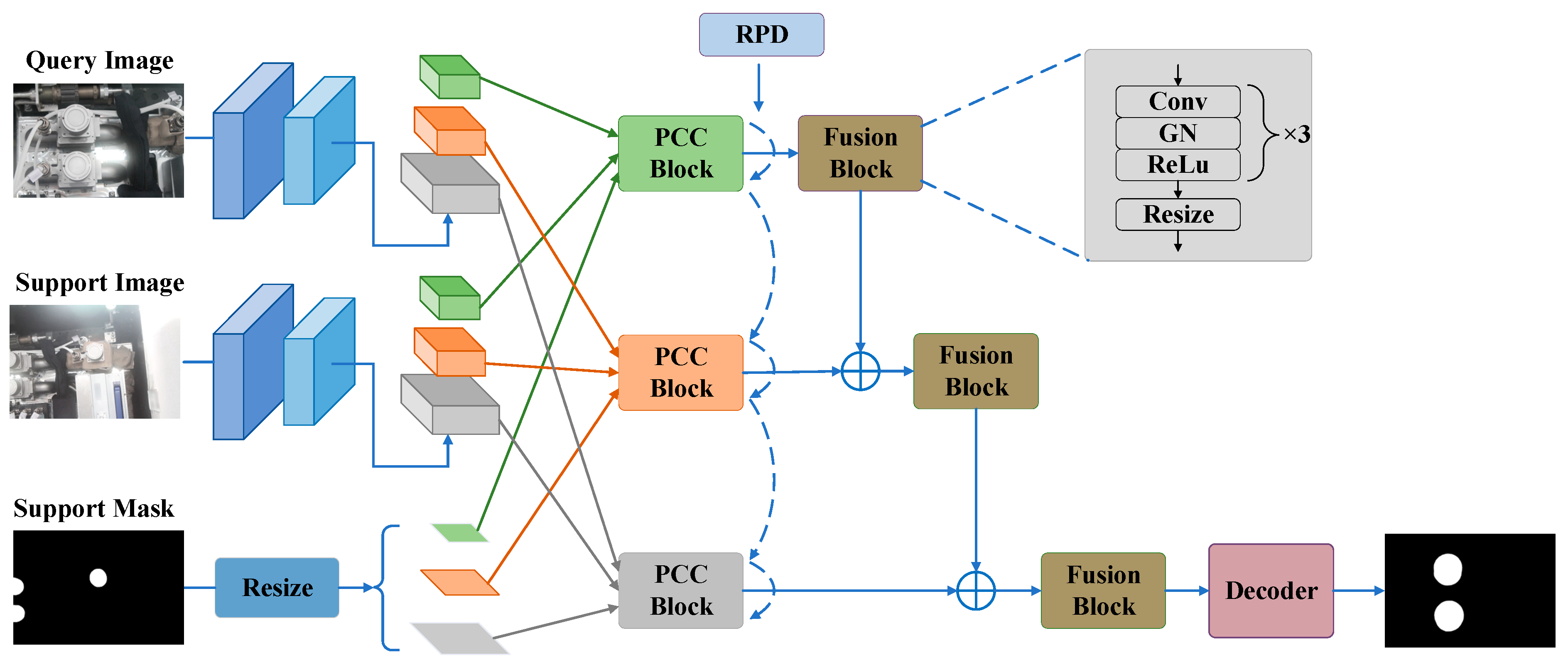
The overall architecture of our PCNet is illustrated in Figure 1. The input of PCNet is a query image and several support images with fine annotated masks. Segmentation of the query image is desired as the output. Firstly, the pre-trained ResNet50 [48] is selected as the shared feature extractor between the support and query paths with frozen parameters. Secondly, in the last three blocks of the backbone, we design novel pixel-wise and class-wise correlation blocks (PCC blocks) for mining dense semantic relationships between support and query features. Specifically, we construct prototypes using support features and corresponding resized masks for each layer in each block. Abstract deep prototypes reverse global semantic cues to shallow layers through distillation (reverse prototype distillation, RPD), forcing shallow prototypes to learn more explicit semantic information. Thirdly, all features of each block are fused using a simple fusion module, and features from multiple blocks are combined by hierarchical fusion. Finally, the results are obtained through a decoder consisting mainly of convolutional and upsampling layers. We will explain our model in detail in the following sections, with a focus on PCC blocks and RPDs under the 1-shot setting.
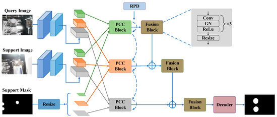
Figure 1.
The overall architecture of the proposed PCNet, including the shared backbone, PCC block, fusion block, RPD module, and a simple decoder. Different colors in the backbone indicate different blocks. Dashed arcs indicate inter-layer RPDs (short arcs) or inter-block RPDs (long arcs). is the pixel-wise addition.
3.3. Feature Preparation
To ensure the generalization of FSS, we follow the standard practice of freezing the backbone. Most published FSS works use features of the last layer of the backbone for post-processing. We are inspired by [42,44] to fully utilize the dense features within every block for feature extraction. The support features and query features are and , respectively, where is the index of blocks. For ResNet50, . The larger is, the deeper the block is. And is the index of layers in each block.
We actually perform the research with valued . In response, the number of layers to each block is , respectively. The scale of layers in the same block is the same, but the scales are different between different blocks. The scales corresponding to these three blocks are of the input image, respectively. For the support mask, we adjust it to the same scale as the features in each block, denoted as .
3.4. Rational Application of the Cross-Attention
Transformers capture contextual relationships between pixels and are widely used for feature extraction [46,47,49]. The core formula of the transformer is as follows:
where are tokens constructed from the feature map, and is the dimension of Q and K. is the affinity map [13], measuring the correlation between Q and K. When come from the same feature map, Equation (1) denotes the self-attention, which is widely used for feature extraction within an image.
One of the critical techniques in FSS is to find the association between the support feature and the query feature. Cross-attention is an effective pixel-wise association method that has been widely used in many studies [12,13,43,44]. The key to cross-attention is that in Equation (1) come from different feature maps. Methods in [12,13] use query features as Q and background-removed support features as K and V, while the support mask is used for background removal only. Such an approach is suitable for natural datasets such as COCO [14] and PASCAL VOC [50], which obtain images with significant inter-class differences and large foreground–background differences. Thus, removing the background before transformers indeed reduces the effect of irrelevant factors.
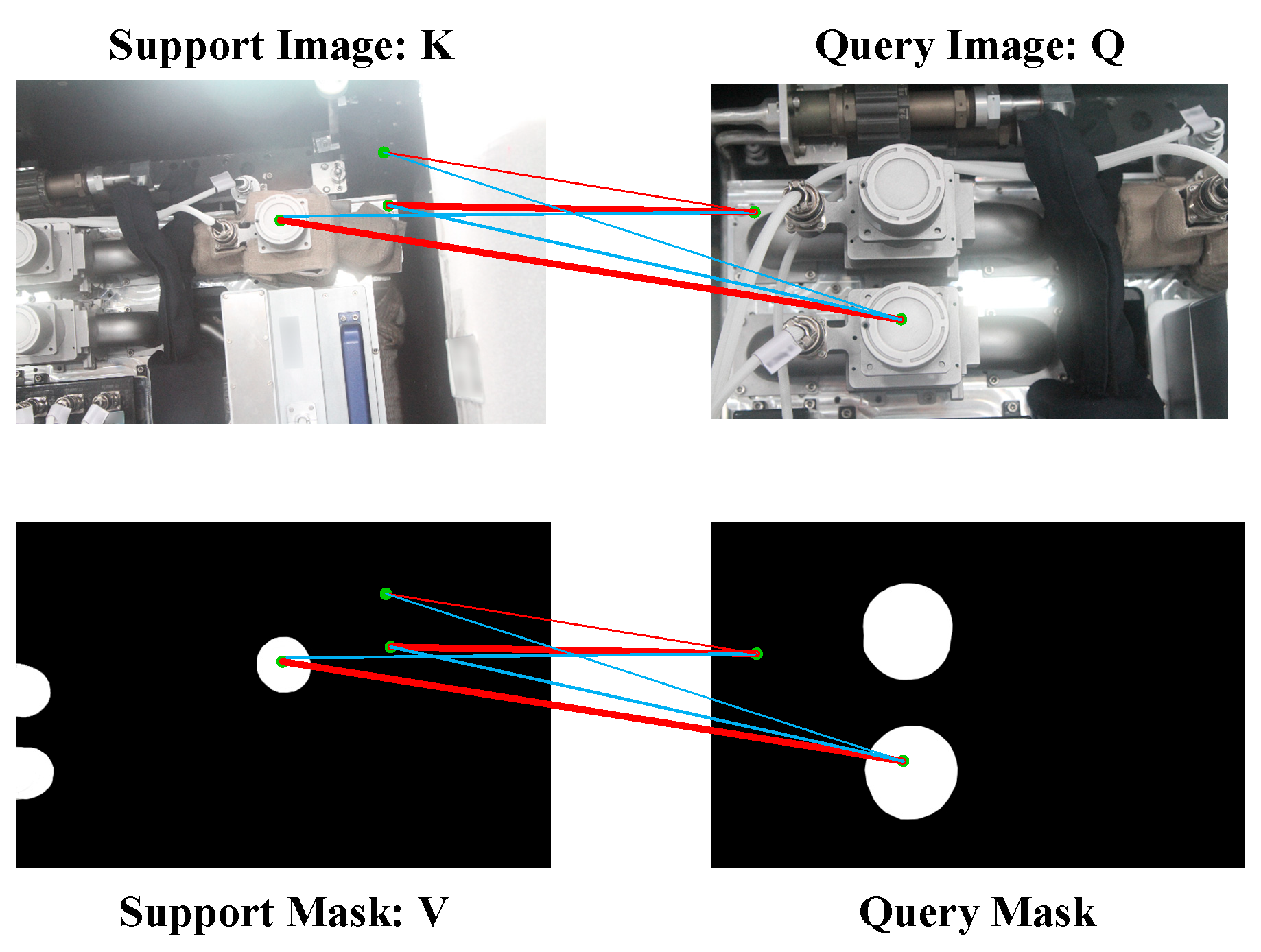
However, for AWS data, the similarity between different categories is significant. The FG and BG of images are easy to confuse. Cross-attention is achieved by flattening the feature map, where each pixel represents a token. The purpose of cross-attention is to find matching relationships on pixels. As shown in Figure 2, for a certain pixel in the support FG, there are similar pixels for both the FG and BG in the query. The cross-attention is calculated by point-wise multiplication. Similar query pixels are multiplied by support FG pixels to yield similar values. Query pixels are multiplied by the support BG to reach the value 0. Therefore, it is difficult to distinguish similar query pixels. The above characteristic of AWSs leads to false segmentation.
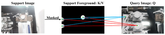
Figure 2.
False segmentation due to the similarity of FG-BG. The blue line indicates that the query BG is correlated with the support FG and is the cause of incorrect segmentation. The red line indicates the correct correlation.
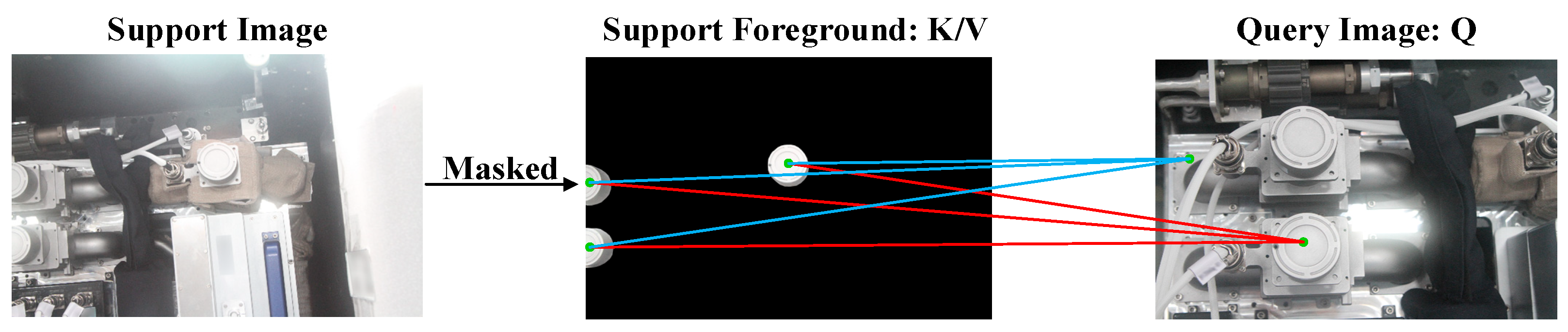
Inspired by DCAMA [44], we adopt another form of cross-attention. As shown in Figure 3, Q, K, and V are query features, support features, and support masks, respectively. We first compute the affinity matrix, , followed by softmax, i.e., , which represents the pixel-wise dense correlation in K and Q. Unlike [12,13], the BG of the support features is also involved in the computation. Therefore, combines the different feature values of FG and BG and their corresponding positional encodings to contain more information. A higher similarity between the support and query features leads to a stronger correlation. The thickness of the lines is used in Figure 3 to indicate the degree of correlation. A weaker correlation between dissimilar features helps to distinguish features that are semantically different but similar in appearance. In addition, we multiply with V, i.e., . The learned correlation is used to weight the support mask to obtain query masks.
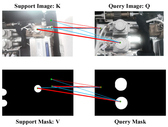
Figure 3.
Cross-attention in our method. The blue line indicates the false correlation. The red line indicates correct correlations. The thicker the line, the stronger the correlation. Correlations calculated between support and query features are transferred to the support mask to predict the query mask.
3.5. Pixel-Wise and Class-Wise Correlation Block (PCC Block)
PCC blocks are implemented in the last three blocks of the backbone. As shown in Figure 4, the 5th block is used as an example to illustrate the proposed module. Support features and query features are denoted as and , respectively. There are three layers inside the block, i.e., . All the layers are scaled to of the input image. We resize support masks to the same scale by linear interpolation to obtain .
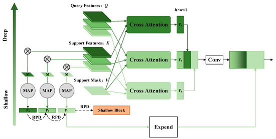
Figure 4.
PCC block modified from the 5th block of ResNet50. Darker colors indicate deeper layers. MAP denotes the masked average pooling. means the Hadamard product. M is the support mask. P is the prototype. RPD stands for reverse prototype distill. Conv includes convolution, group normalization, and ReLu.
We consider the query feature , the support feature , and the support mask of corresponding layers as Q, K, and V, respectively. The corresponding tensor dimensions are and , respectively. The multi-head form is used for computation according to Equation (1), i.e., learning the mapping , where . Then, we stack different layers of in the channel dimension, i.e., . These features are then fused using a convolution operation. With such dense cross-attention, each layer in each block is involved in computation, providing considerable pixel-wise semantic information.
In addition, we construct prototypes for each support layer according to the standard practice [51], which is formulated as follows:
where is the Hadamard product and is the average global pooling. As shown in Figure 4, in the 5th block, three prototypes are constructed to represent the class-wise semantic cues of a particular layer, i.e., the semantic information of the whole category is compressed into a high-dimensional vector. We distill deeper prototypes to shallower layers reversely (which will be explained in the next section). Then, we expand the shallowest prototype and connect it to to obtain the final feature of this block. The whole process is summarized as follows:
where . means concatenation in the channel dimension. includes dense pixel-wise and class-wise semantic cues in the ith block (i is 5 in this example), allowing for detail-to-global feature extraction. Similar operations are performed for features in each block.
3.6. Reverse Prototype Distillation (RPD)
Equation (2) computes the prototype of each layer, compressing the category cues at different stages. Prototypes are characterized by global abstraction and have been used in many studies [8,52,53]. However, some works [13,44] argue that prototypes suffer from information loss.
In this paper, such a class-wise feature is proved to be an effective complement to pixel-wise features, and the two features can realize complementary advantages. Unlike previous work where prototypes are extracted only once, in PCNet, dense prototypes are extracted. Several studies [20,22] point out that deeper features are more abstract and characterize global semantic information. Similarly, the deeper the prototype, the more precise its semantic information. The natural idea is to propagate the prototypes of deeper features to shallower ones, thus enhancing the semantic representation of shallow prototypes.
Specifically, for all prototypes , we first extend them to the same dimension using the fully connected layer, i.e., , where is a fixed value. Next, the softmax layer normalizes prototypes by the following:
where T is the distillation temperature, a hyperparameter which we set to 0.5. The effects caused by different T will be given in ablation studies.
The direction of distillation is opposite to the forward of the backbone, i.e., reverse distillation. The deeper the feature layer is, the stronger its prototype. The prototype of the last layer in the last block is the initial teacher and distills forward sequentially. The KL divergence loss [12] is utilized to supervise the process of distillation, which is formulated as follows:
where n denotes the number of layers in each block, and when . denotes the full distillation loss in each block, as shown by the short-dashed arcs in Figure 1 and the dashed arcs in Figure 4. denotes the full distillation loss from the first layer of the deeper block to the last layer of the shallower block, as shown by the long dashed arcs in Figure 1 and the straight dashed line in Figure 4. It should be noted that the distillation is only performed during training.
3.7. Feature Fusion and Decoder
We use a simple module to fuse pixel-wise and class-wise semantic cues from the PCC block. As shown in Figure 1, the fusion block consists of stacked convolution, group normalization, and ReLu. Then, the feature map is resized so that it has the same scale as the previous block. Inspired by [44], we merge the features of the last three blocks using the progressive union module, which is formalized as follows:
where denotes the fusion block. Finally, is processed by a simple decoder containing mainly convolutional and upsampling layers to obtain the query mask. The overall loss of PCNet is formulated as follows:
where is the binary cross-entropy loss, which is a commonly used loss in many studies [8,12,44]. is set to 1 since we do not find a large improvement in performance with different values.
3.8. Extension to K-Shot Setting
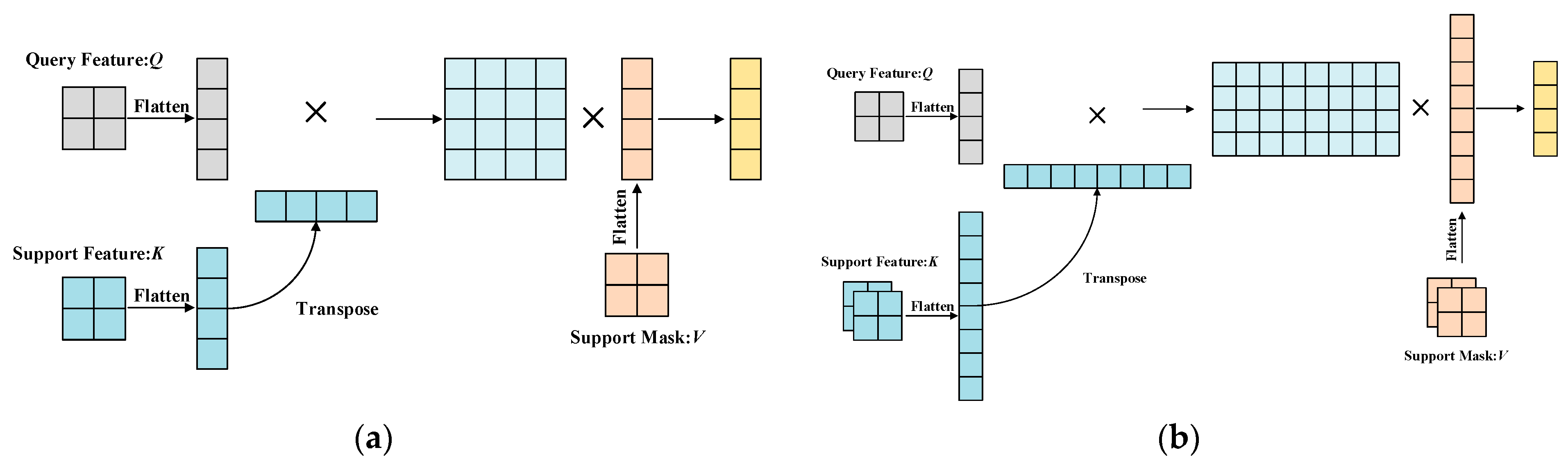
PCNet can be extended to a K-shot (K > 1) model without retraining. As shown in Figure 5a, we flatten the feature map before the cross-attention to obtain tokens. As shown in Figure 5b, under the K-shot setting, we connect the tokens of the K support feature maps to construct tokens. The same operation is applied to the K support masks. Equation (1) is computed using the dot product, which does not require learning and does not change the dimension of the final result. Therefore, this extension can be performed naturally. For K pairs of support data, we use Equation (2) to compute the prototypes at each level. Then, we find the average of the K prototypes. The formulation is calculated as follows:
where is a single prototype created from one support image and its corresponding mask.

Figure 5.
The calculation process of 1-shot and 5-shot settings. (a) The 1-shot setting. (b) The 5-shot setting.
4. Experimental Settings
4.1. Dataset
To meet the experimental needs, we create the semantic segmentation dataset of the CSS. Specifically, we rely on the simulator developed by the China Astronaut Research and Training Center (ACC) to acquire rich images. For objects inside the cabin, a camera is used to capture images of each object at different angles, distances, and scales. We want to simulate the astronauts working inside the CSS from various perspectives and to improve the richness of the dataset. For important objects outside the cabin, we utilize the virtual reality system developed by the ACC to simulate various perspectives outside the cabin in space.
We select 1000 images containing 28 real objects inside the cabin and 8 virtual objects outside the cabin as the final dataset for annotation. To further increase the richness and adaptability of data, the dataset is augmented with random rotation, random flip, random brightness, random exposure, and random saturation. Finally, we obtained 7255 pairs and named them Space Station 36 (SS-36). Among them, the training set contains 4836 images with corresponding masks, and the test set contains 2419 images with corresponding masks. To the best of our knowledge, this is the first AWS dataset applied to SS.
Some samples are shown in Figure 6. As shown in Figure 6a, the distinction between the categories of AWS images is unclear. The FG and BG are easily confused. The effects of light are intense. The FG has fewer textures and occupies a small proportion of pixels. Figure 6c shows the results obtained using the state-of-the-art (SOTA) method [12]. Issues like incomplete segmentation, FG/GB confusion, and missing segmentation are likely to happen. Mainstream FSS methods are unable to handle such complex images effectively.
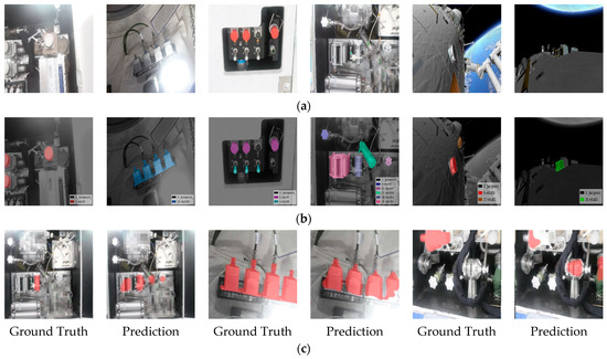
Figure 6.
Characteristics of AWSs. (a) Samples of the dataset. (b) Labels corresponding to the samples. (c) Some predictions using the method from HDMNet [12].
Furthermore, we construct SS-36 into the cross-validation format required by FSS. The training and test sets are divided into four splits. In order to balance the diversity and fairness among categories, each split contains seven in-cabin real objects and two out-of-cabin virtual objects, totaling nine categories. There is no category overlap between the four splits. We named this dataset SS-9i.
The training is performed on three of the splits, and the testing is performed on another split. Thus, four experiments need to be performed, which is known as the cross-validation in FSS.
4.2. Metrics
Two metrics [8,12] are used in our experiments:
Equation (11) is the mean intersection over union (mIoU), where is the number of categories. Equation (12) is the average of the IoU of the FG and the IoU of the BG.
4.3. Implementation Details
We normalize the input images to uniform 400 × 400 pixels and do not perform any further data enhancement, similar to previous works [42,44]. To ensure the generalization of the model, we fix the parameters of the backbone. It should be noted that using different backbones will result in different performances [13,43,52]. However, we mainly verify the performance of the proposed core modules. Therefore, only ResNet50 is chosen for our experiments. The same backbone is chosen for all the comparison models. We conduct experiments on 2080Ti GPUs using the PyTorch framework. For training, the batch size, initial learning rate, momentum, and weight decay are set to 8, 0.001, 0.9, and 0.0001, respectively. The SGD optimizer is used until the model converges. During testing, we randomly select 500 samples, and the average is the final result.
5. Results and Discussion
5.1. Comparison with the SOTA Methods
In this work, eight typical models from recent years are adopted for comparison. Two of them are based on prototypes [8,52], and six on pixel-wise semantic matching [12,13,42,43,44,45]. All models are based on ResNet50. All models are retrained on SS-9i with original settings until they converge. It is worth noting that the leading models, BAM [8] and HDMNet [12], use additional branches for base classes. Specifically, the base path is first trained, and then the backbone of the base branch is used for the second stage. However, using the backbone trained with the base branch is equivalent to fine-tuning it on the target dataset, unlike most models that fix the backbone. Therefore, it is not fair to use this approach for comparison. Among experiments, both results for this two-stage training and one-stage training with a fixed backbone are illustrated.
Table 1 shows the results of PCNet and some mainstream methods in comparison. The best results are highlighted in bold, while suboptimal results are underlined. It can be seen that PCNet achieves optimal results in almost all settings, and only Split3 achieves suboptimal results under the 1-shot setting. The closest match to PCNet is DCAMA [44], which achieves suboptimal results in most of the results. Our method outperforms DCAMA by 4.34% and 5.15% under the 1-shot and 5-shot settings, respectively.

Table 1.
Quantitative results on ss-9i. The metric used is mIoU (%). Best results are bolded, and sub-optimal results are underlined. “*” indicates that the backbone of the model is pre-trained by ImageNet.
For two special methods, BAM and HDMNet, the results obtained with the pre-trained backbone are significantly worse than those obtained by fine-tuning the backbone on SS-9i. BAM shows a reduction of 11.21% and 12.40% under 1-shot and 5-shot settings, respectively. HDMNet has decreases of 10.95% and 8.79%, respectively. The reason for such significant differences is that AWSs are very different from natural data. Therefore, the backbone fine-tuned by SS-9i is more suitable for AWSs. It is not fair to compare with other models using such a trick. Even with the pre-trained backbone, our proposed method greatly outperforms BAM and HDMNet. Compared with HDMNet, the SOTA method on nature data, the mIoU of PCNet is 24.50% and 31.34% higher under 1-shot and 5-shot settings, respectively.
From another perspective, class-based methods [8,52] are inferior to pixel-wise methods [12,13,42,44,45,54]. In addition, pixel-wise methods are further divided into three categories: methods based on 4D convolutions [42,45], methods using cross-attention between the query image and support images [12,13,43] only, and methods taking masks into cross-attention [44]. PCNet belongs to the third category. The second category gives the worst results, while the third category gives the best results, which proves the effectiveness of the method proposed.
In addition, we calculate the FB-IOU and inference speed of various models. As shown in Table 2, our model still shows the highest accuracy, outperforming DCAMA by 1.03% and 2.01% under 1-shot and 5-shot settings, respectively. The inference speed of pixel-wise methods is much lower than that of class-wise methods due to the intensive computation consumption by the pixel-wise form. PCNet ranks fourth among the pixel-wise methods, lower than BAM, DCAMA, and HSNet.
Table 2.
Quantitative results using FB-IoU and FPS as metrics. Best results are bolded, and sub-optimal results are underlined. “*” indicates that the backbone of the model is pre-trained by ImageNet.
5.2. Qualitative Results
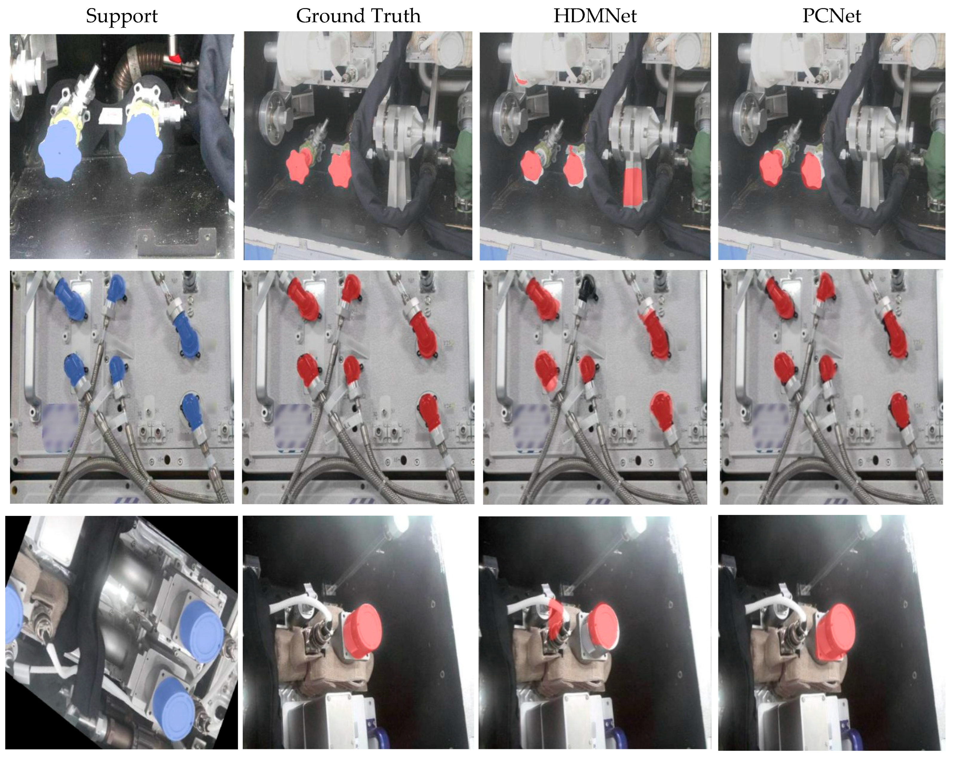
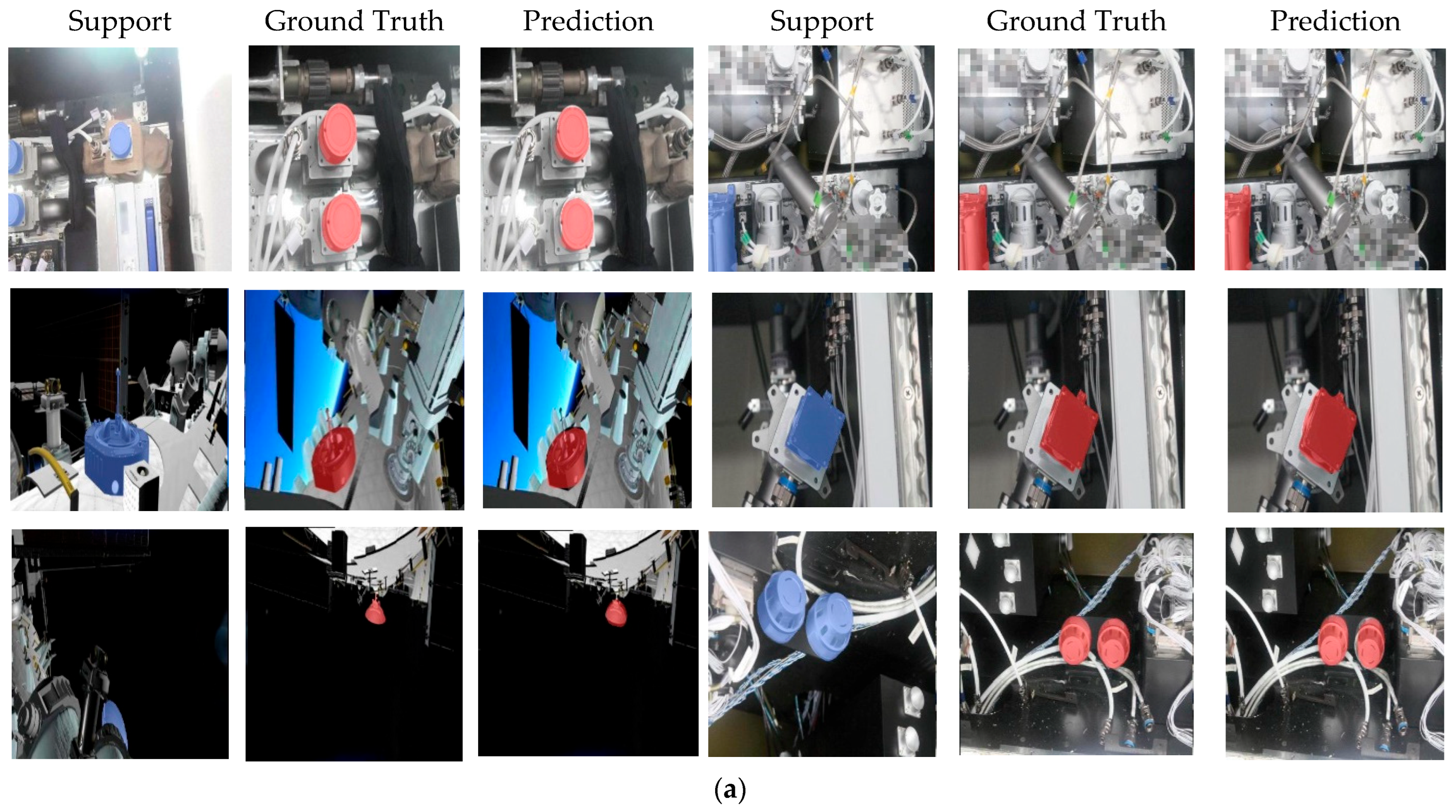
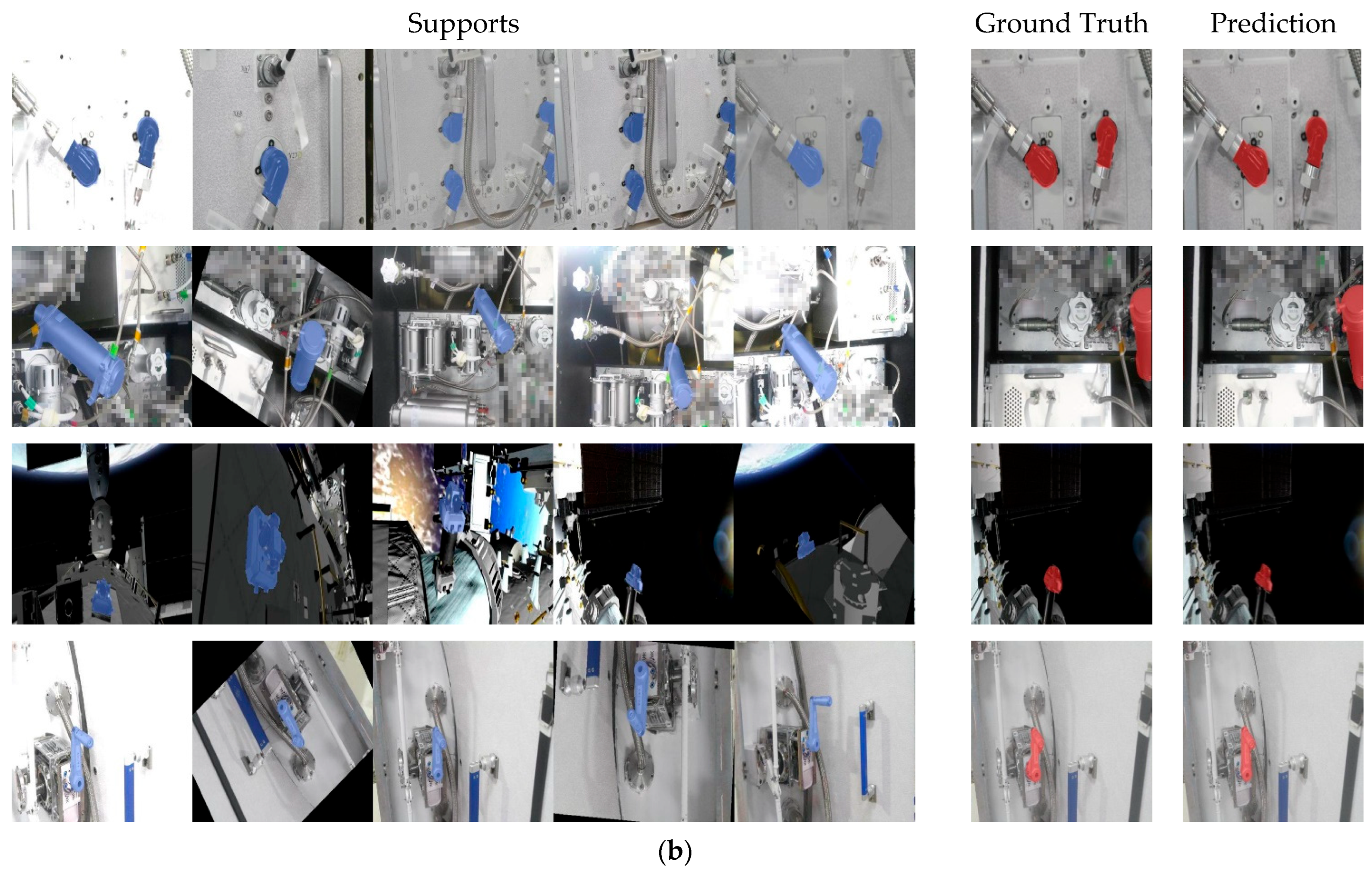
Figure 7 shows a visual comparison between HDMNet and PCNet under the 1-shot setting. Although HDMNet is a SOTA method on natural datasets, it does not work well on AWS images, providing few correct and complete segmentations. In contrast, PCNet works much better because of its unique specifications for AWS data. Figure 8 shows the visualization of PCNet under 1-shot and 5-shot settings. Similar to most FSS methods, the segmentation becomes better as support cues increase in amount.
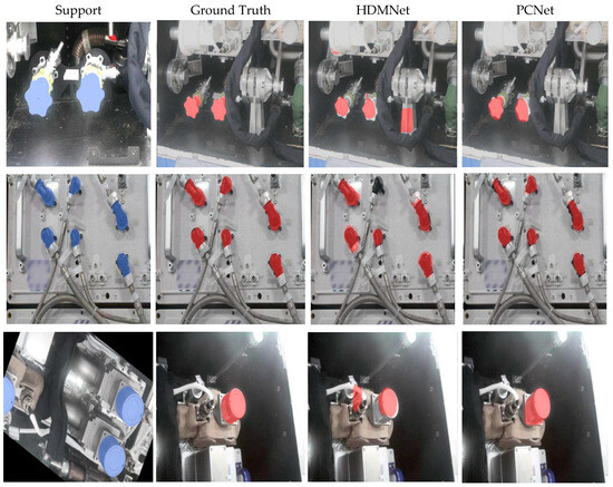
Figure 7.
Comparison of qualitative results between HDMNet and PCNet.
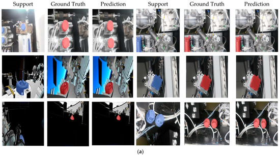
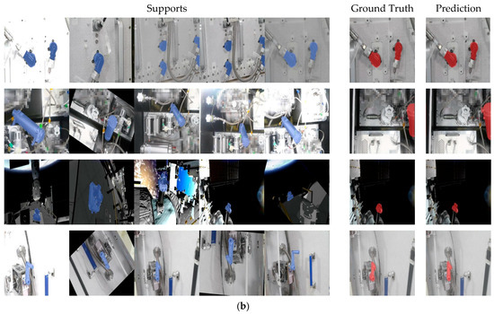
Figure 8.
Comparison of qualitative results with PCNet under different settings. (a) Results under the 1-shot setting. (b) Results under the 5-shot setting.
5.3. Ablation Studies
In order to demonstrate the effect of the proposed modules and hyperparameters used, we perform ablation studies. For brevity, the experiments are performed only under the 1-shot setting. Compared with FB-IoU, mIoU reflects the performance of the model more accurately. Therefore, we adopt mIoU as the metric in most of the experiments.
5.3.1. Effects of the Proposed Modules
As shown in Table 3, we validate the effect of the two main modules, PCC and RPD. The baseline is the architecture without dense prototypes and reverse prototype distillation, where the PCC module uses only dense cross-attention. No RPD means no prototype distillation. It can be seen that the average mIoU of all four splits increases by 4.34% with the usage of dense prototypes. In addition, the performance improves by 7.77% with the addition of RPD. These results demonstrate the effectiveness of using such class-wise semantic cues.
Table 3.
Ablation studies of the proposed modules. “Prototype” means using dense prototypes in cross-attention. “RPD” denotes the reverse prototype distillation. Best results are bolded, and sub-optimal results are underlined.
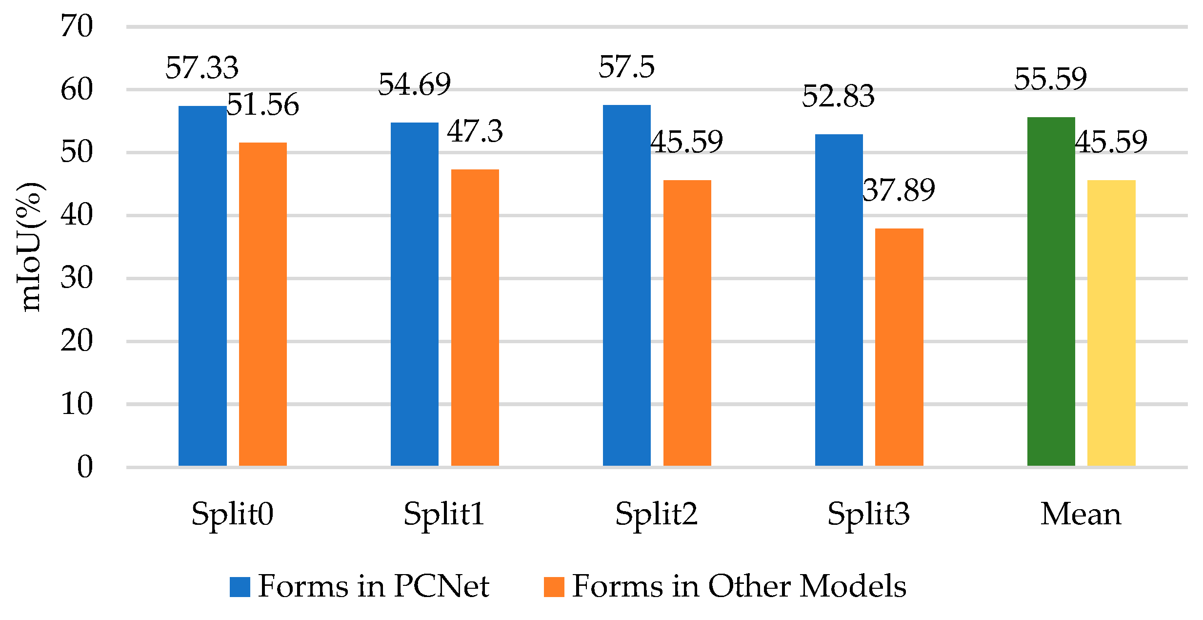
5.3.2. Effects of Different Forms of Cross-Attention
Some FSS methods [12,13,43] use cross-attention for pixel-wise matching between support features and query features. These methods first multiply support features with support masks. As explained in Chapter 2.3, removing the foreground yields the masked support features, which are used in cross-attention as K and V. It is worth noting that instead of using dense cross-attention inside the block, other methods [12,13,43] use cross-attention at the last layer of each block. For fairness, we modify their architecture to the same dense form as ours. As shown in Figure 9, our method outperforms the other methods significantly, improving the average accuracy by 21.93%. These results prove that the method proposed in our work is more applicable to AWS data.
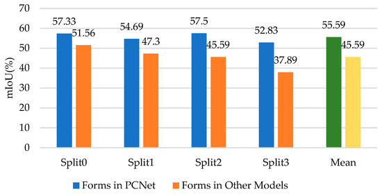
Figure 9.
Ablation studies of different forms of cross-attention.
5.3.3. Effects of the Distillation Temperature
The distillation temperature T in Equation (4) is a hyperparameter that affects the results. We choose T = {0.5, 1, 2, 3} for experiments. As shown in Table 4, when T equals 0.5, the average accuracy of all four splits is the highest. PCNet adopts the value 0.5. However, we can also find that the variation in T shows a weak influence on results, and the best result (T equals 0.5) is only 2.60% higher than the worst result (T equals 3).
Table 4.
Ablation studies of different distillation temperatures. Best results are bolded, and sub-optimal results are underlined.
5.3.4. SS vs. FSS
We compare the gap between FSS and SS. PSPNet is chosen as the SS method, a widely used model, which is used as the base branch in [8,12]. As support features increase, memory usage gradually increases. To lower computation consumption, we resize the size of input images to 350 × 350. For PSPNet, we use standard supervised learning to train and test each split. For FSS, we conduct cross-validation by selecting shot = {1, 5, 8, 10, 12, 13, 14, 15}.
As shown in Table 5, PSPNet has the highest accuracy in Split1 and Split2 but did not perform as well as in the other two splits. In Split0, the mIoU of PSPNet is only higher than that of PCNet under the 1-shot setting. With an increase in support data, PCNet’s mIoU is higher than PSPNet’s. In Split3, the accuracy of PSPNet is comparable to that of PSPNet under the 5-shot setting. Compared to FSS, PSPNet shows an unevenly distributed accuracy across the different groups due to the smaller categories in both Split0 and Split3. Traditional semantic segmentation has a weaker ability to deal with small objects. It is important to note that PSPNet [55] has an mIoU of 85.40 for PASCAL VOC and 80.20 for Cityscapes but only 65.91 for AWS data, proving that AWSs are challenging scenes.
Table 5.
Comparison between SS and FSS. Best results are bolded, and sub-optimal results are underlined.
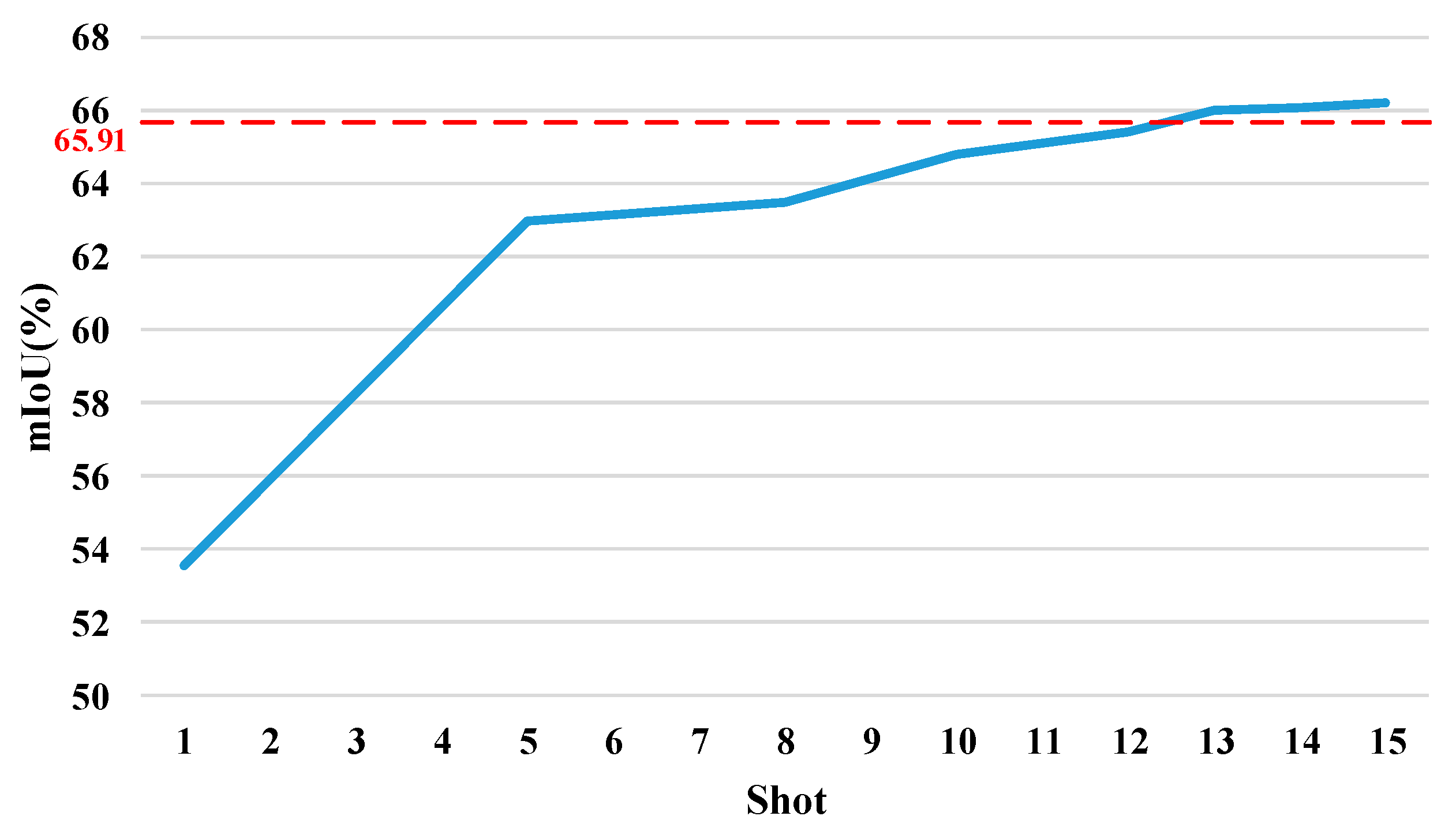
Figure 10 shows the average accuracy across all four splits with different amounts of support data. The red dotted line is the result of PSPNet. For FSS, the mIoU has increased significantly from the 1-shot to the 5-shot setting, increasing by 17.61%. However, the curve from the 5-shot to the 15-shot setting is relatively flat, with a growth rate of 5.14%. In particular, when the number of support features is greater than 10, the improvement in accuracy is slower. From the 10-shot to 15-shot setting, the accuracy increases by only 2.21%. While PCNet’s accuracy surpasses PSPNet after the 13-shot setting, the increment is small. The 15-shot setting is only 0.47% more accurate than PSPNet. After the 15-shot setting, it does not make much sense for FSS, so it can be assumed that the PCNet’s accuracy is stable at the same level as PSPNet.
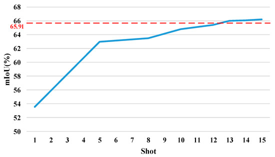
Figure 10.
Average mIoU over four splits under different settings. The red dotted line is the result of PSPNet. The blue line shows the results for PCNet with a different amount of support data.
SS-9i contains 100 to 137 samples per class. The accuracy achieved by PSPNet using more than 100 samples can be achieved with only 13 samples for PCNet. What is more, with PCNet, there is no need to train on unseen categories. This conclusion proves that the proposed method can reduce annotations in amount and can be applied to untrained classes.
6. Conclusions
The special layout of AWSs poses a great challenge to the segmentation supported by a small number of annotations. We propose a dedicated and efficient model, PCNet, to solve this issue. Specifically, PCNet is mainly composed of two modules: PCC and RPD. The former uses unique cross-attention and dense prototypes to extract complementary semantic associations between support and query features pixel-wise and class-wise, respectively. The latter reversely distills deep prototypes to shallow layers to improve the quality of their corresponding prototypes. To verify the effectiveness of our proposed method and facilitate the engineering application, we customize a dataset for AWSs. Experiments show that PCNet exceeds current leading FSS methods in accuracy. An accuracy increase is achieved as 4.34% and 5.15% more than the suboptimal model under 1-shot and 5-shot settings, respectively. Further experiments show that PCNet matches the traditional semantic segmentation method in accuracy under the 13-shot setting. It is noted that FSS methods, such as PCNet, can handle untrained classes, breaking the limitation of traditional semantic segmentation. In summary, PCNet shows both academic and engineering significance, accelerating the development of AWS intelligent parsing.
Author Contributions
Conceptualization, Q.S. and J.C.; methodology, Q.S. and W.L.; investigation, Z.X., D.W. and W.C.; writing—original draft preparation, Q.S.; writing—review and editing, D.W., W.C. and S.X.; visualization, Z.X. and S.X.; supervision, J.C.; funding acquisition, W.L. All authors have read and agreed to the published version of the manuscript.
Funding
This research was funded by the Work Enhancement Based on Visual Scene Perception.
Data Availability Statement
The data presented in this study are available on request from the corresponding author. The data are not publicly available due to privacy restrictions.
Conflicts of Interest
The authors declare no conflicts of interest.
References
- Bertrand, R. Conceptual design and flight simulation of space stations. Aerosp. Sci. Technol. 2001, 5, 147–163. [Google Scholar] [CrossRef]
- Li, D.; Liu, H.; Sun, Y.; Qin, X.; Hu, X.; Shi, L.; Liu, Q.; Wang, Y.; Cheng, T.; Yi, D.; et al. Active Potential Control Technology of Space Station and Its Space-ground Integrated Verification. J. Astronaut. 2023, 44, 1613–1620. [Google Scholar] [CrossRef]
- Wang, K.; Zhang, B.; Xing, T. Preliminary integrated analysis for modeling and optimizing space stations at conceptual level. Aerosp. Sci. Technol. 2017, 71, 420–431. [Google Scholar] [CrossRef]
- Shi, L.; Yao, H.; Shan, M.; Gao, Q.; Jin, X. Robust control of a space robot based on an optimized adaptive variable structure control method. Aerosp. Sci. Technol. 2022, 120, 107267. [Google Scholar] [CrossRef]
- Yuan, H.; Cui, Y.; Shen, X.; Liu, Y.; Wang, Z.; Zhang, L.; Zhang, C.; Shi, F. Technology and Development of Sub-System of Docking and Transposition Mechanism for Space Station Laboratory Module. Aerosp. Shanghai (Chin. Engl.) 2023, 40, 71–77. [Google Scholar] [CrossRef]
- Shelhamer, E.; Long, J.; Darrell, T. Fully Convolutional Networks for Semantic Segmentation. IEEE Trans. Pattern Anal. Mach. Intell. 2017, 39, 640–651. [Google Scholar] [CrossRef] [PubMed]
- Pan, Z.; Jiang, P.; Wang, Y.; Tu, C.; Cohn, A.G. Scribble-Supervised Semantic Segmentation by Uncertainty Reduction on Neural Representation and Self-Supervision on Neural Eigenspace. In Proceedings of the IEEE/CVF International Conference on Computer Vision (ICCV), Montreal, QC, Canada, 10–17 October 2021; pp. 7396–7405. [Google Scholar] [CrossRef]
- Lang, C.; Cheng, G.; Tu, B.; Han, J. Learning What Not to Segment: A New Perspective on Few-Shot Segmentation. In Proceedings of the IEEE/CVF Conference on Computer Vision and Pattern Recognition (CVPR), New Orleans, LA, USA, 18–24 June 2022; pp. 8047–8057. [Google Scholar] [CrossRef]
- Shaban, A.; Bansal, S.; Liu, Z.; Essa, I.; Boots, B. One-Shot Learning for Semantic Segmentation. arXiv 2017, arXiv:1709.03410. [Google Scholar]
- Vinyals, O.; Blundell, C.; Lillicrap, T.; Kavukcuoglu, K.; Wierstra, D. Matching Networks for One Shot Learning. In Proceedings of the International Conference on Neural Information Processing Systems (NeurlPS), Barcelona, Spai, 5–10 December 2016; pp. 3637–3645. [Google Scholar]
- Yang, B.; Liu, C.; Li, B.; Jiao, J.; Ye, Q. Prototype Mixture Models for Few-shot Semantic Segmentation. In Proceedings of the European Conference on Computer Vision (ECCV), Glasgow, UK, 23–28 August 2020. [Google Scholar] [CrossRef]
- Peng, B.; Tian, Z.; Wu, X.; Wang, C.; Liu, S.; Su, J.; Jia, J. Hierarchical Dense Correlation Distillation for Few-Shot Segmentation. In Proceedings of the IEEE/CVF Conference on Computer Vision and Pattern Recognition (CVPR), Vancouver, BC, Canada, 17–24 June 2023; pp. 23641–23651. [Google Scholar] [CrossRef]
- Zhang, G.; Kang, G.; Yang, Y.; Wei, Y. Few-Shot Segmentation via Cycle-Consistent Transformer. In Proceedings of the International Conference on Neural Information Processing Systems (NeurIPS), Online, 6–14 December 2021; pp. 21984–21996. [Google Scholar]
- Lin, T.-Y.; Maire, M.; Belongie, S.; Hays, J.; Perona, P.; Ramanan, D.; Dollár, P.; Zitnick, C.L. Microsoft COCO: Common Objects in Context. In Proceedings of the European Conference on Computer Vision (ECCV), Zurich, Switzerland, 6–12 September 2014; pp. 740–755. [Google Scholar] [CrossRef]
- Chen, L.-C.; Zhu, Y.; Papandreou, G.; Schroff, F.; Adam, H. Encoder-Decoder with Atrous Separable Convolution for Semantic Image Segmentation. In Proceedings of the European Conference on Computer Vision (ECCV), Munich, Germany, 8–14 September 2018; pp. 833–851. [Google Scholar] [CrossRef]
- Yuan, Y.; Chen, X.; Wang, J. Object-Contextual Representations for Semantic Segmentation. In Proceedings of the European Conference on Computer Vision (ECCV), Cham, Switzreland, 23–28 August 2020; pp. 173–190. [Google Scholar] [CrossRef]
- Badrinarayanan, V.; Kendall, A.; Cipolla, R. SegNet: A Deep Convolutional Encoder-Decoder Architecture for Image Segmentation. IEEE Trans. Pattern Anal. Mach. Intell. 2017, 39, 2481–2495. [Google Scholar] [CrossRef]
- Chen, J.; Lu, Y.; Yu, Q.; Luo, X.; Adeli, E.; Wang, Y.; Lu, L.; Yuille, A.L.; Zhou, Y. TransUNet: Transformers Make Strong Encoders for Medical Image Segmentation. arXiv 2021, arXiv:2102.04306. [Google Scholar]
- Howard, A.G.; Zhu, M.; Chen, B.; Kalenichenko, D.; Wang, W.; Weyand, T.; Andreetto, M.; Adam, H. MobileNets: Efficient Convolutional Neural Networks for Mobile Vision Applications. arXiv 2017, arXiv:1704.04861. [Google Scholar]
- Yu, C.; Wang, J.; Peng, C.; Gao, C.; Yu, G.; Sang, N. BiSeNet: Bilateral Segmentation Network for Real-Time Semantic Segmentation. In Proceedings of the European Conference on Computer Vision (ECCV), Munich, Germany, 8–14 September 2018; pp. 334–349. [Google Scholar] [CrossRef]
- Yu, C.; Gao, C.; Wang, J.; Yu, G.; Shen, C.; Sang, N. BiSeNet V2: Bilateral Network with Guided Aggregation for Real-Time Semantic Segmentation. Int. J. Comput. Vision 2021, 129, 3051–3068. [Google Scholar] [CrossRef]
- Fan, M.; Lai, S.; Huang, J.; Wei, X.; Chai, Z.; Luo, J.; Wei, X. Rethinking BiSeNet For Real-time Semantic Segmentation. In Proceedings of the IEEE/CVF Conference on Computer Vision and Pattern Recognition (CVPR), Nashville, TN, USA, 20–25 June 2021; pp. 9711–9720. [Google Scholar] [CrossRef]
- Hu, J.; Shen, L.; Albanie, S.; Sun, G.; Wu, E. Squeeze-and-Excitation Networks. IEEE Trans. Pattern Anal. Mach. Intell. 2020, 42, 2011–2023. [Google Scholar] [CrossRef]
- Woo, S.; Park, J.; Lee, J.-Y.; Kweon, I.S. CBAM: Convolutional Block Attention Module. In Proceedings of the Computer Vision—ECCV 2018, Cham, Switzerland, 8–14 September 2018; pp. 3–19. [Google Scholar] [CrossRef]
- Xie, E.; Wang, W.; Yu, Z.; Anandkumar, A.; Alvarez, J.M.; Luo, P. SegFormer: Simple and Efficient Design for Semantic Segmentation with Transformers. In Proceedings of the International Conference on Neural Information Processing Systems (NeurIPS), New Orleans, LA, USA, 6–14 December 2021; pp. 12077–12090. [Google Scholar]
- Li, W.; Wang, L.; Xu, J.; Huo, J.; Gao, Y.; Luo, J. Revisiting Local Descriptor Based Image-To-Class Measure for Few-Shot Learning. In Proceedings of the 2019 IEEE/CVF Conference on Computer Vision and Pattern Recognition (CVPR), Long Beach, CA, USA, 15–20 June 2019; pp. 7253–7260. [Google Scholar] [CrossRef]
- Qiao, L.; Shi, Y.; Li, J.; Tian, Y.; Huang, T.; Wang, Y. Transductive Episodic-Wise Adaptive Metric for Few-Shot Learning. In Proceedings of the 2019 IEEE/CVF International Conference on Computer Vision (ICCV), Seoul, Republic of Korea, 27 October–2 November 2019; pp. 3602–3611. [Google Scholar] [CrossRef]
- Wu, Z.; Li, Y.; Guo, L.; Jia, K. PARN: Position-Aware Relation Networks for Few-Shot Learning. In Proceedings of the 2019 IEEE/CVF International Conference on Computer Vision (ICCV), Seoul, Republic of Korea, 27 October–2 November 2019; pp. 6658–6666. [Google Scholar] [CrossRef]
- Ye, H.J.; Hu, H.; Zhan, D.C.; Sha, F. Few-Shot Learning via Embedding Adaptation With Set-to-Set Functions. In Proceedings of the 2020 IEEE/CVF Conference on Computer Vision and Pattern Recognition (CVPR), Seattle, WA, USA, 13–19 June 2020; pp. 8805–8814. [Google Scholar] [CrossRef]
- Li, H.; Eigen, D.; Dodge, S.; Zeiler, M.; Wang, X. Finding Task-Relevant Features for Few-Shot Learning by Category Traversal. In Proceedings of the 2019 IEEE/CVF Conference on Computer Vision and Pattern Recognition (CVPR), Long Beach, CA, USA, 15–20 June 2019; pp. 1–10. [Google Scholar] [CrossRef]
- Jamal, M.A.; Qi, G.J. Task Agnostic Meta-Learning for Few-Shot Learning. In Proceedings of the 2019 IEEE/CVF Conference on Computer Vision and Pattern Recognition (CVPR), Long Beach, CA, USA, 15–20 June 2019; pp. 11711–11719. [Google Scholar] [CrossRef]
- Chen, Z.; Fu, Y.; Wang, Y.X.; Ma, L.; Liu, W.; Hebert, M. Image Deformation Meta-Networks for One-Shot Learning. In Proceedings of the 2019 IEEE/CVF Conference on Computer Vision and Pattern Recognition (CVPR), Long Beach, CA, USA, 15–20 June 2019; pp. 8672–8681. [Google Scholar] [CrossRef]
- Zhang, C.; Lin, G.; Liu, F.; Yao, R.; Shen, C. CANet: Class-Agnostic Segmentation Networks With Iterative Refinement and Attentive Few-Shot Learning. In Proceedings of the IEEE/CVF Conference on Computer Vision and Pattern Recognition (CVPR), Long Beach, CA, USA, 15–20 June 2019; pp. 5212–5221. [Google Scholar] [CrossRef]
- Dong, N.; Xing, E.P. Few-Shot Semantic Segmentation with Prototype Learning. In Proceedings of the British Machine Vision Conference, Northumbria, UK, 3–6 September 2018; p. 79. [Google Scholar]
- Fan, Q.; Pei, W.; Tai, Y.-W.; Tang, C.-K. Self-support Few-Shot Semantic Segmentation. In Proceedings of the European Conference on Computer Vision (ECCV), Tel Aviv, Israel, 23–27 October 2022; pp. 701–719. [Google Scholar] [CrossRef]
- Luo, X.; Tian, Z.; Zhang, T.; Yu, B.; Tang, Y.Y.; Jia, J. PFENet++: Boosting Few-Shot Semantic Segmentation With the Noise-Filtered Context-Aware Prior Mask. IEEE Trans. Pattern Anal. Mach. Intell. 2023, 46, 1273–1289. [Google Scholar] [CrossRef] [PubMed]
- Tian, Z.; Lai, X.; Jiang, L.; Liu, S.; Shu, M.; Zhao, H.; Jia, J. Generalized Few-shot Semantic Segmentation. In Proceedings of the 2022 IEEE/CVF Conference on Computer Vision and Pattern Recognition (CVPR), New Orleans, LA, USA, 18–24 June 2022; pp. 11553–11562. [Google Scholar] [CrossRef]
- Wang, K.; Liew, J.H.; Zou, Y.; Zhou, D.; Feng, J. PANet: Few-Shot Image Semantic Segmentation With Prototype Alignment. In Proceedings of the 2019 IEEE/CVF International Conference on Computer Vision (ICCV), Seoul, Republic of Korea, 27 October–2 November 2019; pp. 9196–9205. [Google Scholar] [CrossRef]
- Li, G.; Jampani, V.; Sevilla-Lara, L.; Sun, D.; Kim, J.; Kim, J. Adaptive Prototype Learning and Allocation for Few-Shot Segmentation. In Proceedings of the 2021 IEEE/CVF Conference on Computer Vision and Pattern Recognition (CVPR), Nashville, TN, USA, 20–25 June 2021; pp. 8330–8339. [Google Scholar] [CrossRef]
- Zhang, C.; Lin, G.; Liu, F.; Guo, J.; Wu, Q.; Yao, R. Pyramid Graph Networks With Connection Attentions for Region-Based One-Shot Semantic Segmentation. In Proceedings of the 2019 IEEE/CVF International Conference on Computer Vision (ICCV), Seoul, Republic of Korea, 27 October–2 November 2019; pp. 9586–9594. [Google Scholar] [CrossRef]
- Lu, Z.; He, S.; Zhu, X.; Zhang, L.; Song, Y.Z.; Xiang, T. Simpler is Better: Few-shot Semantic Segmentation with Classifier Weight Transformer. In Proceedings of the IEEE/CVF International Conference on Computer Vision (ICCV), Montreal, QC, Canada, 10–17 October 2021; pp. 8721–8730. [Google Scholar] [CrossRef]
- Min, J.; Kang, D.; Cho, M. Hypercorrelation Squeeze for Few-Shot Segmenation. In Proceedings of the IEEE/CVF International Conference on Computer Vision (ICCV), Montreal, QC, Canada, 10–17 October 2021; pp. 6921–6932. [Google Scholar] [CrossRef]
- Xu, Q.; Zhao, W.; Lin, G.; Long, C. Self-Calibrated Cross Attention Network for Few-Shot Segmentation. In Proceedings of the IEEE/CVF International Conference on Computer Vision (ICCV), Paris, France, 1 August 2023; pp. 655–665. [Google Scholar] [CrossRef]
- Shi, X.; Wei, D.; Zhang, Y.; Lu, D.; Ning, M.; Chen, J.; Ma, K.; Zheng, Y. Dense Cross-Query-and-Support Attention Weighted Mask Aggregation for Few-Shot Segmentation. In Proceedings of the European Conference on Computer Vision (ECCV), Tel Aviv, Israel, 23–27 October 2022; pp. 151–168. [Google Scholar] [CrossRef]
- Liu, H.; Peng, P.; Chen, T.; Wang, Q.; Yao, Y.; Hua, X.S. FECANet: Boosting Few-Shot Semantic Segmentation with Feature-Enhanced Context-Aware Network. IEEE Trans. Multimed. 2023, 25, 8580–8592. [Google Scholar] [CrossRef]
- Vaswani, A.; Shazeer, N.; Parmar, N.; Uszkoreit, J.; Jones, L.; Gomez, A.N.; Kaiser, L.; Polosukhin, I. Attention Is All You Need. In Proceedings of the International Conference on Neural Information Processing Systems (NeurIPS), Red Hook, NY, USA, 4–9 December 2017; pp. 6000–6010. [Google Scholar]
- Liu, Z.; Lin, Y.; Cao, Y.; Hu, H.; Wei, Y.; Zhang, Z.; Lin, S.; Guo, B. Swin Transformer: Hierarchical Vision Transformer using Shifted Windows. In Proceedings of the 2021 IEEE/CVF International Conference on Computer Vision (ICCV), Montreal, BC, Canada, 10–17 October 2021; pp. 9992–10002. [Google Scholar] [CrossRef]
- He, K.; Zhang, X.; Ren, S.; Sun, J. Deep Residual Learning for Image Recognition. In Proceedings of the IEEE Conference on Computer Vision and Pattern Recognition (CVPR), Las Vegas, NV, USA, 27–30 June 2016; pp. 770–778. [Google Scholar] [CrossRef]
- Dosovitskiy, A.; Beyer, L.; Kolesnikov, A.; Weissenborn, D.; Zhai, X.; Unterthiner, T.; Dehghani, M.; Minderer, M.; Heigold, G.; Gelly, S.; et al. An Image is Worth 16x16 Words: Transformers for Image Recognition at Scale. arXiv 2020, arXiv:2010.11929. [Google Scholar]
- Everingham, M.; Gool, L.V.; Williams, C.K.; Winn, J.; Zisserman, A. The pascal visual object classes (voc) challenge. Int. J. Comput. Vis. 2010, 88, 303–338. [Google Scholar] [CrossRef]
- Zhang, X.; Wei, Y.; Yang, Y.; Huang, T.S. SG-One: Similarity Guidance Network for One-Shot Semantic Segmentation. IEEE Trans. Cybern. 2020, 50, 3855–3865. [Google Scholar] [CrossRef] [PubMed]
- Tian, Z.; Zhao, H.; Shu, M.; Yang, Z.; Li, R.; Jia, J. Prior Guided Feature Enrichment Network for Few-Shot Segmentation. IEEE Trans. Pattern Anal. Mach. Intell. 2022, 44, 1050–1065. [Google Scholar] [CrossRef] [PubMed]
- Lang, C.; Wang, J.; Cheng, G.; Tu, B.; Han, J. Progressive Parsing and Commonality Distillation for Few-Shot Remote Sensing Segmentation. IEEE Trans. Geosci. 2023, 61, 1–10. [Google Scholar] [CrossRef]
- Zhang, B.; Xiao, J.; Qin, T. Self-Guided and Cross-Guided Learning for Few-Shot Segmentation. In Proceedings of the 2021 IEEE/CVF Conference on Computer Vision and Pattern Recognition (CVPR), Nashville, TN, USA, 20–25 June 2021; pp. 8308–8317. [Google Scholar] [CrossRef]
- Zhao, H.; Shi, J.; Qi, X.; Wang, X.; Jia, J. Pyramid Scene Parsing Network. In Proceedings of the IEEE Conference on Computer Vision and Pattern Recognition (CVPR), Piscataway, NJ, USA, 21–26 July 2017; pp. 6230–6239. [Google Scholar] [CrossRef]


Disclaimer/Publisher’s Note: The statements, opinions and data contained in all publications are solely those of the individual author(s) and contributor(s) and not of MDPI and/or the editor(s). MDPI and/or the editor(s) disclaim responsibility for any injury to people or property resulting from any ideas, methods, instructions or products referred to in the content. |
© 2024 by the authors. Licensee MDPI, Basel, Switzerland. This article is an open access article distributed under the terms and conditions of the Creative Commons Attribution (CC BY) license (https://creativecommons.org/licenses/by/4.0/).