Article

RANS-Based Aerodynamic Shape Optimization of a Wing with a Propeller in Front of the Wingtip

by
Shamsheer S. Chauhan
* and
Joaquim R. R. A. Martins
Department of Aerospace Engineering, University of Michigan, Ann Arbor, MI 48109, USA
*
Author to whom correspondence should be addressed.
Aerospace 2024, 11(7), 512; https://doi.org/10.3390/aerospace11070512
Submission received: 23 April 2024 / Revised: 15 June 2024 / Accepted: 18 June 2024 / Published: 25 June 2024
(This article belongs to the Section Aeronautics)

Abstract

:
Accounting for propeller–wing interaction allows for the design of more efficient propeller aircraft through strategic propulsion integration. In this paper, the cruise drag of a wing with a propeller located in front of the wingtip is minimized using twist and airfoil-shape design variables. Reynolds-averaged Navier–Stokes computational fluid dynamics with an actuator-disk approach is used for the flow simulations, and a gradient-based algorithm is used for the optimization. Changing the rotation direction of the propeller and optimizing the twist and airfoil shapes of the wing are found to impact the aerodynamic performance significantly, as expected. However, optimizing the wing while accounting for the propeller slipstream during optimization provides little benefit over optimizing it without accounting for the propeller slipstream—a difference of less than one drag count.

1. Introduction

Recent electric aircraft development efforts have led to a renewed focus on the design and optimization of propeller aircraft [1,2,3,4,5,6,7,8,9,10,11,12,13,14,15,16,17]. Electric motors allow for easier distribution of the propulsion on an aircraft than combustion engines, allowing for the design of more efficient propeller aircraft through strategic propulsion integration [1,3].
When a propeller is located near a wing, the flow induced by it affects the lift and drag of the wing [18,19,20,21,22,23,24,25]. The effects change with the location and rotation direction of the propeller [18,21,22,23,24,25]. When a propeller is located directly in front of a wing, its axial and tangential induced-velocity components cause spanwise variations in the local angles of attack and effective freestream speeds of the wing sections. This affects the lift and drag of the sections immediately behind the propeller as well as of the rest of the wing [24,25]. The disturbed flow behind a propeller can also increase boundary-layer turbulence over the wing and cause cycling between laminar and turbulent transitional states [26]. The static-pressure gradients in the slipstream also influence boundary layer development. When a propeller is located directly behind a wing, its influence on the wing is significantly weaker because of lower propeller-induced velocities and the absence of propeller-induced swirl in front of the propeller [24,27]. Additionally, as Prandtl [18] concluded in an early study, when a propeller is vertically offset relative to a wing, the pressure and velocity distributions associated with streamtube contraction can also affect the wing’s performance.
The flow induced by a wing and other changes to the flow caused by viscous drag or blockage also affect the performance of the propeller [18,22,23,24,27]. This is primarily due to the altered inflow to the propeller and can result in a gain or loss in performance depending on the propeller’s location and rotation direction [18,22,23,24,27]. Generally, the impact on the performance of the propeller is more significant when it is located behind a wing.
Many approaches of varying complexity and fidelity have been used to model propeller–wing interaction [3,6,9,10,11,13,22,23,24,27,28,29,30,31,32,33,34,35,36,37,38,39,40,41]. One approach is to combine a vortex-lattice method (VLM) model for the wing with a propeller model that provides induced velocities, such as a blade-element momentum model [9,10,13,24,29,30,36]. This approach has limitations related to thickness and viscous effects and requires correction factors to accurately model the influence of a propeller’s slipstream on a wing [9,13,24,36]. Another approach, which captures these effects more directly, is to model a propeller as an actuator disk in a steady computational fluid dynamics (CFD) simulation by distributing time-averaged propeller forces over a disk using force terms (momentum source terms) or boundary conditions [3,6,24,27,28,32,34,37,39,40,42]. Another related approach is to use rotating actuator lines that represent the blades in an unsteady CFD simulation [37]. To capture more detail, another approach is to use unsteady CFD with resolved three-dimensional blade geometry [27,33,34,37,38]. However, these unsteady approaches result in a significantly higher computational cost, which is prohibitive for optimization.
The approach of using steady CFD with an actuator disk has been shown to provide accurate time-averaged predictions for a wing located behind a propeller [17,24,32,34,37]. Although the flow induced by a propeller is fundamentally unsteady, unsteady CFD approaches provide little additional accuracy for time-averaged lift and drag, assuming that accurate propeller loading distributions are available [24,32,34,37,38]. Therefore, a steady actuator-disk approach is a suitable and more tractable option for RANS-based design optimization.
There are a small number of prior published studies on optimizing wings while accounting for propeller–wing interaction. Kroo [22] presented a study on lift-distribution optimization to minimize the induced losses of a wing with an inboard propeller. The optimized lift distributions deviate from the elliptical shape that is ideal for an isolated wing. Additionally, the optimized lift distributions for inboard-up, outboard-up, and counter-rotating propellers differ significantly. Kroo [22] also concluded that losses associated with swirl may be recovered with equal increases in efficiency for both tractor and pusher configurations. The limitations of the approach used by Kroo [22] include the low fidelity of the models (a lifting-line approach with an idealized helical propeller wake), neglecting viscous effects, and optimizing the lift distribution instead of geometric design parameters.
Veldhuis and Heyma [31] presented optimization results for a rectangular wing with an inboard tractor propeller with the objective of minimizing drag subject to a lift constraint using wing-twist design variables. They used a lifting-line approach with a viscous-drag estimation method for the wing and induced-velocity models for the propeller. Their results show negligible differences in drag between minimizing only the induced drag and minimizing the sum of the induced and viscous drag, as expected, because only twist design variables were used. They also optimized a wing based on the Fokker 50 (inboard tractor propeller) at a cruise condition and predicted induced-drag reductions of 13 drag counts for inboard-up rotation and 8 drag counts for outboard-up rotation relative to an optimized wing with no propeller. Their optimized wings have increased twist behind the down-going-blade region and decreased twist behind the up-going-blade region. The limitations of their approach include the low fidelity of the models and the limited design freedom. Rakshith et al. [35] used a similar approach to carry out chord and twist optimization studies for a wing with an inboard tractor propeller. They concluded that it is beneficial to reduce the chord lengths behind the propeller, and they predicted drag reductions between 2% and 12% for varying combinations of flight conditions, constraints, and number of design variables.
Alba et al. [9] developed a model for coupled propeller–wing interaction and optimized a wing with planform and airfoil-shape design variables. They modeled the wing using a quasi-3-D VLM approach and the propeller using XROTOR. They included weight and performance models for a multidisciplinary study. For an aircraft based on the Tecnam P2012 (inboard tractor propeller), their results predict fuel savings of up to 7% relative to the baseline design. They concluded that modifying wing twist and camber to align the wing sections with the propeller swirl is beneficial. The limitations of their approach include the use of low-fidelity models and the limited number of design variables. Epema [36] also presented chord and twist optimization studies for a wing using similar models for the propeller–wing interaction, and they conducted wind tunnel experiments to validate their simulation approaches.
Pedreiro [42] presented an optimization study for a wing with an inboard tractor propeller, based on the Embraer EMB-120, using RANS CFD with an actuator-disk approach and a blade-element model for the propeller loads. Six design variables were used with a design-of-experiments (DOE) approach to optimize the twist and airfoil shapes of the wing segment behind the propeller, and a drag reduction of 3 drag counts was predicted for a cruise condition. Unlike the previous studies, the lowest-drag design obtained by Pedreiro [42] does not have a lower twist behind the up-going-blade region and a higher twist behind the down-going-blade region. A limitation of the approach used by Pedreiro [42] is that the number of design variables and the ability to carry out a large number of optimization studies are severely limited because of the poor scaling of DOE approaches with the number of design variables.
To address the aforementioned limitations of the prior work with regard to the fidelity of the models and the ability to explore the design space, we previously developed the capability to perform gradient-based aerodynamic shape optimization using RANS CFD with an actuator-disk approach [17] using the MACH framework [43]. In a previous paper [17], we presented a series of aerodynamic shape optimization results for a wing with an inboard tractor propeller using gradient-based optimization to answer how important optimizing the wing while accounting for the propeller slipstream is. We found that optimizing the wing while accounting for the propeller slipstream provides little benefit over optimizing it without accounting for the propeller slipstream (a difference of less than one drag count). This paper presents the second part of that work, in which we investigate the same for a wing with a propeller located in front of the wingtip. When a propeller is located in front of a wingtip instead of inboard, it interacts more directly with the flow around the wingtip, resulting in a greater influence on the induced velocities on the wing and, consequently, the induced drag. However, only one half of the wingtip propeller’s streamtube impinges on the trailing wing. Therefore, there are differences in the propeller–wing interaction that motivate this separate study for them.
More recently, after the present work was completed, Koyuncuoglu and He [39] continued this project and developed the capability to carry out gradient-based optimization studies using both wing and propeller-model design variables with the same optimization framework as this work but with a different CFD tool, DAFoam, which supports unstructured meshes. They used the same baseline geometry and a similar actuator-disk approach as this work and found that simultaneously optimizing the wing twist, wing airfoil shapes, propeller diameters, and propeller locations provided up to 11% additional drag reduction relative to optimizing only the wing. Their optimized propellers for both twin-propeller and quad-propeller configurations are smaller, closer to the wingtip, and farther in front of the wing relative to the initial design. The majority of the additional drag reductions are due to changes to the spanwise locations of the propellers.
In this paper, we present a series of aerodynamic shape optimization results for a wing with a propeller located in front of the wingtip. We use RANS CFD and gradient-based optimization to answer how important it is to account for the propeller slipstream while optimizing the wing twist and airfoil shapes for such a configuration. We use the same approach that we used previously for an inboard-propeller configuration [17].

2. Computational Tools

Numerical optimization with RANS CFD and a large number of design variables (about 200 in this work) requires a multidisciplinary framework that is both computationally efficient and gradient-based to make the problem tractable. Therefore, we use the open-source MDO of Aircraft Configurations with High Fidelity (MACH) framework [43] (https://github.com/mdolab/MACH-Aero; accessed on 20 April 2024) for this work.

2.1. Flow Solver

For this study, we use the open-source RANS CFD solver ADflow [44,45] (version v2.2.0) and modify it to implement an actuator-disk propeller model. ADflow is a second-order-accurate finite-volume CFD solver that solves the RANS equations on structured multiblock meshes, and it supports overset meshes by using implicit hole cutting [46,47,48]. ADflow uses the Green–Gauss approach for viscous fluxes, and we select the Jameson–Schmidt–Turkel scheme with scalar dissipation [49] for inviscid fluxes. We carry out steady simulations with the Spalart–Allmaras (SA) [50] turbulence model. The SA implementation used here is the SA-noft2 variant described in the NASA Turbulence Modeling Resource (https://turbmodels.larc.nasa.gov/spalart.html; accessed on 20 April 2024), and the production term is computed using a strain formulation. To solve the governing equations, we use the approximate Newton–Krylov solver [44] as the startup strategy before switching to the Newton–Krylov solver, and we converge the total residual norm by eight or more orders of magnitude.
ADflow uses a discrete adjoint implementation via automatic differentiation to efficiently compute the derivatives of the functions of interest with respect to large numbers of design variables [51]. This has enabled RANS-based optimization studies for a wide range of applications [17,45,52]. For this work, we re-differentiate the ADflow code using the automatic differentiation tool Tapenade [53,54] (version 3.10) to account for the variables and computations added for the actuator-disk propeller model. Even though the propeller-model inputs do not depend on the flow variables and are not used as design variables in this study, it is necessary to re-differentiate the code because they appear in the partial derivatives needed to compute the total derivatives.

2.2. Geometry Parameterization

We use MACH’s geometry manipulation module pyGeo [55] (version v1.2.0) to parameterize and modify the wing shape using a free-form deformation (FFD) approach. In this approach, the surface of the wing is embedded in a grid of control points that map to the surface using a B-spline mapping. This allows the surface to be deformed in a continuous manner that gives the optimizer control over the twist and airfoil shapes. For this study, we specify a maximum spline order of four, which means that fourth-order splines are used if the dimensions allow.

2.3. Mesh Movement

We use MACH’s mesh warping module IDWarp [52] (version v2.2.0) to deform the volume mesh as the surface geometry changes during optimization. IDWarp uses an inverse distance weighting method [56] that helps preserve the quality of the mesh as the surface is deformed.

2.4. Optimizer

We use SNOPT [57] (version 7.2-5) to solve the optimization problems. SNOPT is a gradient-based optimizer that uses a sequential quadratic programming algorithm and is designed to handle large-scale nonlinear optimization problems with thousands of constraints and design variables. It has been shown to be effective at solving RANS-based aerodynamic shape optimization problems [17,45,52,58]. SNOPT is wrapped with the open-source package pyOptSparse [59,60] (version v2.1.3) for use with the MACH framework. The major optimality and feasibility tolerances for SNOPT are set to 10 5 for all the optimization cases in this paper, and all the optimization cases finished successfully. To put these tolerances into perspective, for these optimization cases, the objective function changes by less than 0.1% over the last order of convergence of the optimality.

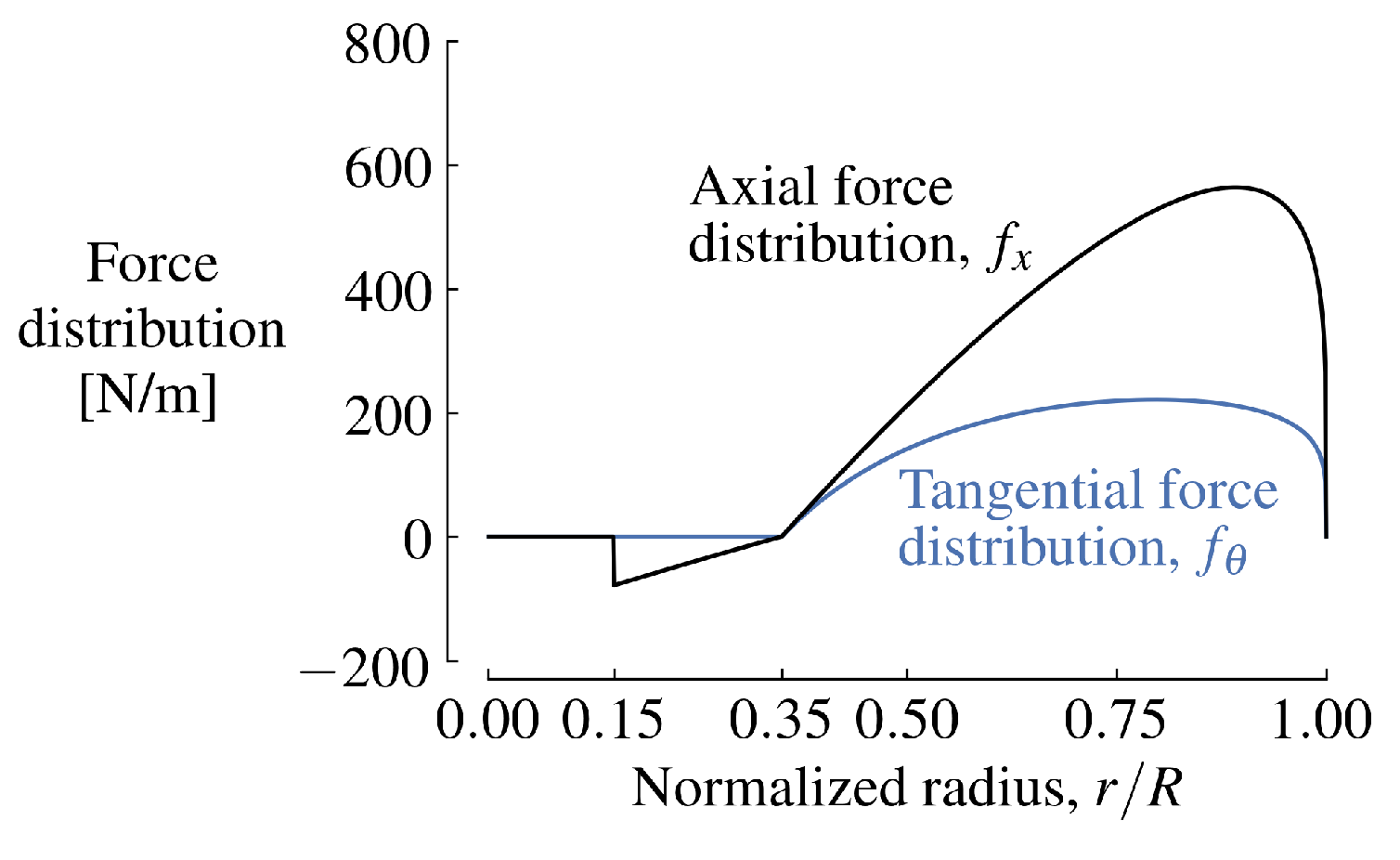
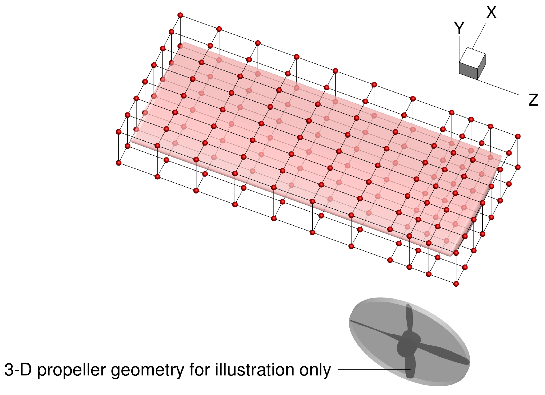
2.5. Propeller Model

We model the propeller using an actuator-disk approach in which forces equal and opposite to time-averaged propeller loads are applied to volume cells in a specified region in the same manner as body forces [17,28]. The model adds terms to both the momentum and energy equations.
Propeller loads can be obtained from various sources, such as analytical models [61,62], blade-element methods [34], or CFD simulations [37]. We use the following models [61] for the distributions of the axial and tangential loading. The radial distribution of the axial force is given by
f x = F r ^ ( 1 r ^ ) n ,
where f x is the axial force per unit radius, r ^ is defined by Equation (2), n is a parameter that is used to adjust the shape of the distribution, and F is a value computed by integrating this distribution over the radius and equating it to the total thrust. Decreasing n shifts the location of maximum thrust towards the tip. The normalized radius r ^ is defined as
r ^ = r r in R r in ,
where r is the radial distance from the axis of rotation, r in is the inner radius of the blades, and R is the outer radius of the propeller. The radial distribution of the tangential force is given by
f θ = f x P / D π ( r / R ) ,
where f θ is the tangential force per unit radius, and P / D is the propeller pitch-to-diameter ratio.
Since Equations (1) and (3) provide continuous distributions, we calculate the forces for each cell in the specified region using their volumes and the distances of their cell centers to the specified propeller axis (i.e., r). The axial and tangential forces per unit volume used for this are given by f x / ( 2 π r t ) and f θ / ( 2 π r t ) , where t is the total thickness of the disk of volume cells to which the forces are applied.

3. Validation Cases

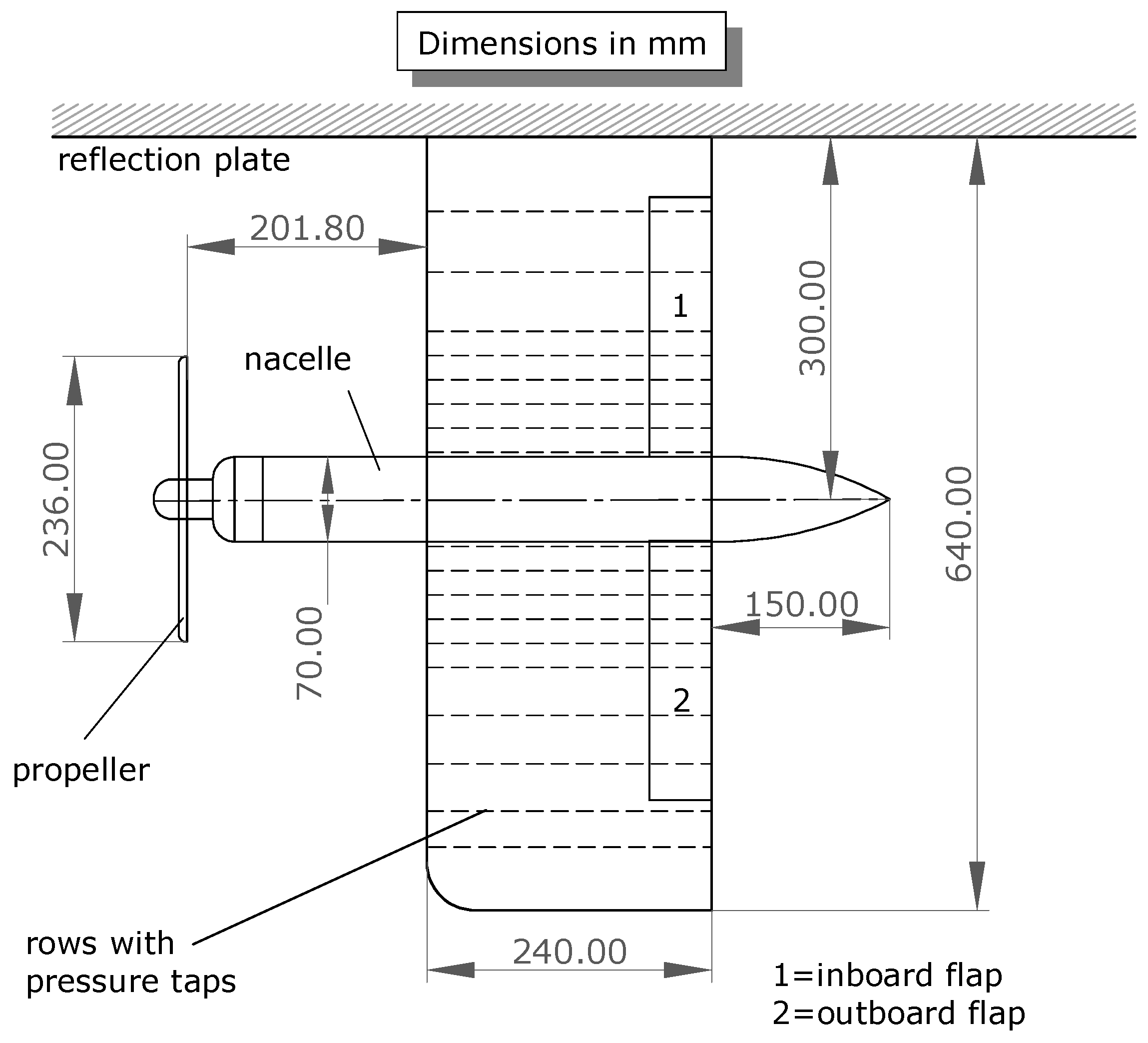
3.1. Geometry and Specifications

We use two experimental cases from Veldhuis [24] to validate our implementation of the propeller model. The configuration is a rectangular wing with a tractor propeller mounted near the midspan, as shown in Figure 1. The wing is not swept, twisted, or tapered. The propeller axis is aligned with the wing section’s chordline and has no vertical offset. The wing airfoil is NACA 642-A015, and we use coordinates from the online UIUC database (https://m-selig.ae.illinois.edu/ads/coord/n64015a.dat; accessed on 1 March 2019). pySpline and pyGeo modules (version v1.2.0 for both) to generate the surface geometry, which is shown in Figure 2a. We do not model the nacelle, nor do we round the leading edge of the wingtip.
We compare our CFD results with experimental data for 0 ° and 4 ° angle-of-attack cases. For these validation simulations, we change the angle of attack by changing the direction of the freestream velocity, so the relative orientations of the actuator disk and the wing are maintained. The Reynolds number and freestream dynamic pressure reported for these cases are 0.8 · 10 6 and 1500 Pa, respectively [24]. For the fluid properties, we use standard sea-level values. The propeller operates with an inboard-up rotation at an advance ratio of J = V / ( ν D ) = 0.85 and a thrust coefficient of T C = T / ( ρ V 2 D 2 ) = 0.168 [24]. Here, V is the freestream speed, ν is the rotation rate, D is the propeller diameter, ρ is the freestream density, and T is the propeller thrust. Veldhuis [24] noted that T C is estimated using a bookkeeping approach (i.e., measuring forces with and without the propeller on) as well as pressure measurements.
We previously presented validation results for this model in an earlier paper [17]. However, we later discovered that we had used an incorrect definition for T C and, consequently, incorrect propeller settings for the results presented there. Updated validation results using the correct T C definition are presented here.

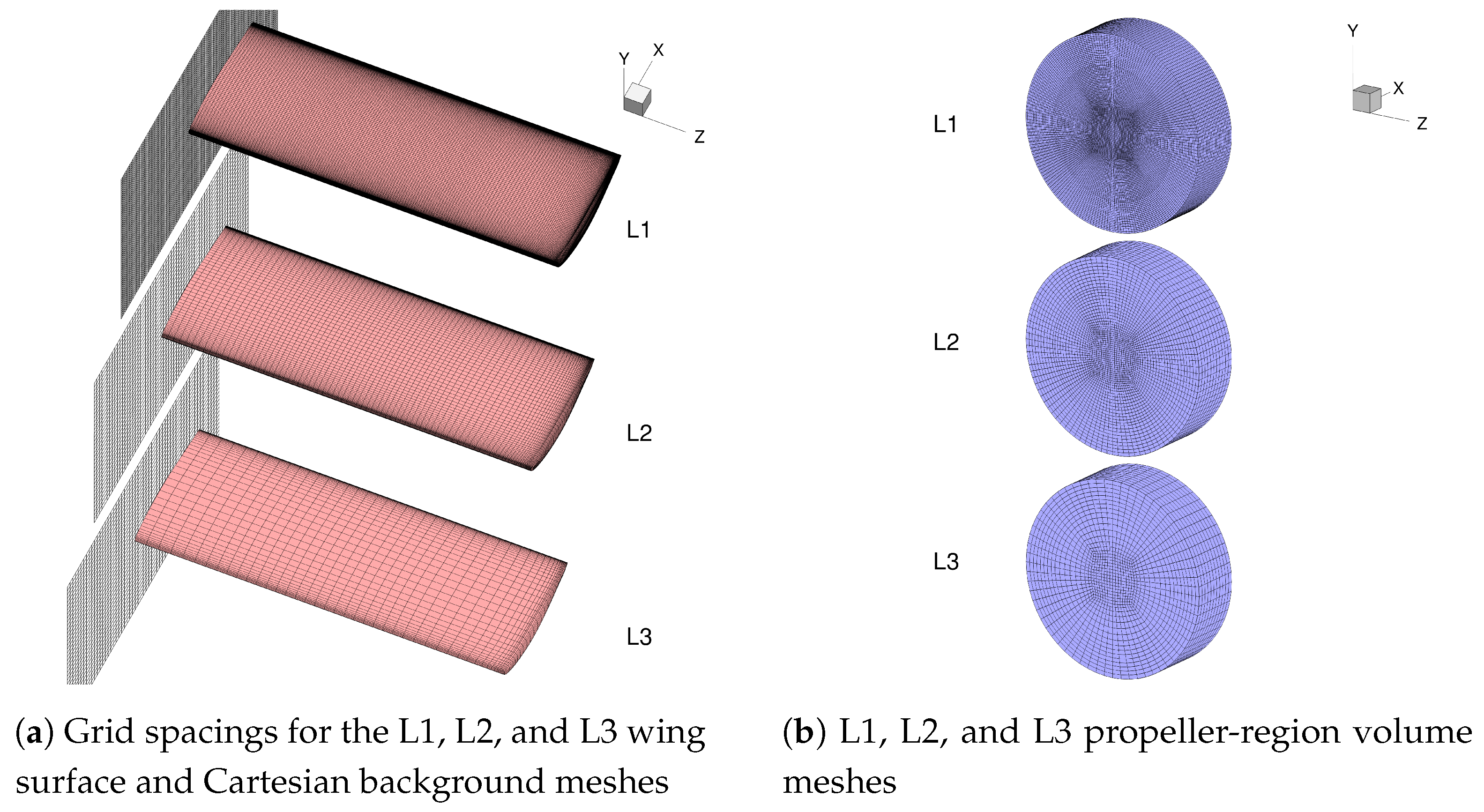
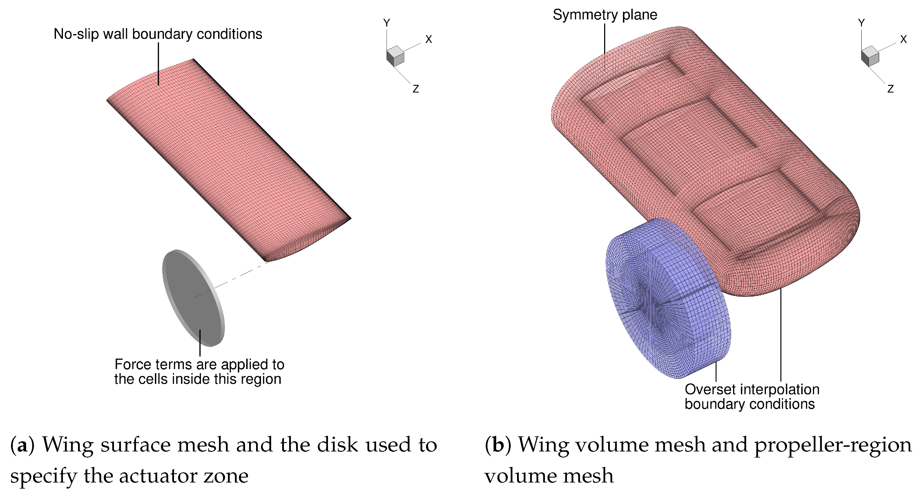
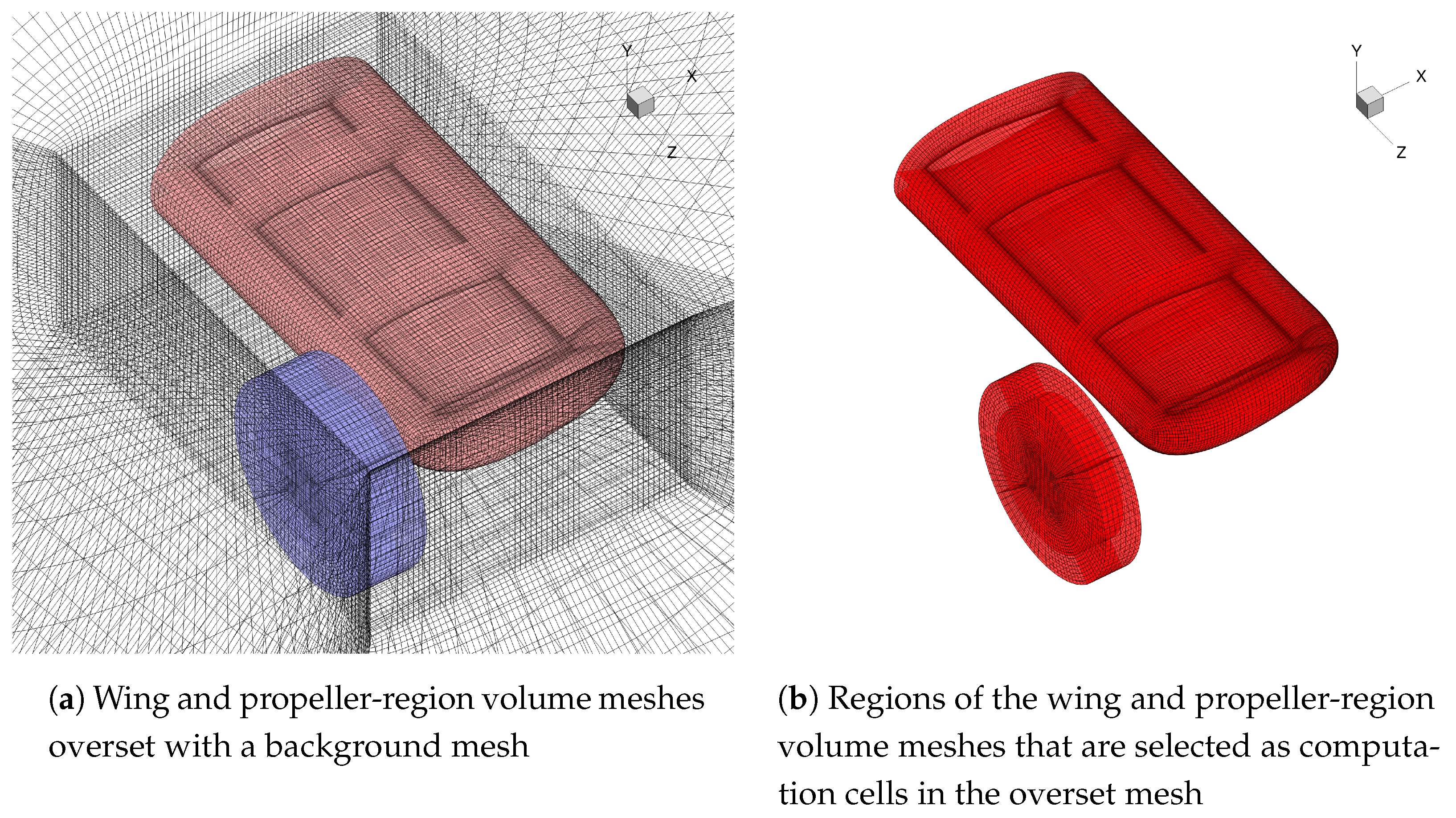
3.2. CFD Volume Meshes

We use three mesh refinement levels named Level 1 (L1), Level 2 (L2), and Level 3 (L3), where the L1 mesh is the finest. For the propeller region, we use a structured multiblock cylindrical volume mesh. The outlines of the blocks of this cylindrical volume mesh are shown in Figure 2b for the L2 refinement. Forces are applied to the cells in this cylindrical mesh that lie inside the disk shown in Figure 2a. The wing surface mesh for the L2 refinement, generated using the commercial package ICEM-CFD, is also shown in Figure 2a. The wing also has a structured multiblock volume mesh, as shown in Figure 2b. The wing volume meshes are generated by extruding the wing surface meshes using MACH’s pyHyp [52] module (version v2.2.0).
The wing and propeller-region volume meshes are overset with a background mesh (Figure 3a). The background mesh consists of a Cartesian volume mesh encapsulating the wing and propeller-region meshes. The outer surfaces of this Cartesian grid are extruded by 45 chord lengths to yield a hemispherical domain. We use far-field boundary conditions for the outer hemispherical surface of this domain and symmetry boundary conditions for the plane coincident with the root of the wing. The propeller-region volume mesh is larger than the disk to which the actuator forces are applied (Figure 2) to allow it to be overset with this background mesh. ADflow uses an implicit hole cutting method for assembling the overset meshes [46,47,48]. The computation cells (i.e., the cells used for the CFD solution and not as fringe cells for interpolation) for the wing and propeller-region volume meshes are shown in Figure 3b for the L2 refinement.
The midplane of the cells that are selected for the actuator zone is located 0.2 m in front of the wing. The radius of the actuator zone is the propeller radius of 0.12 m, and its thickness is 9 mm. A circular disk of cells one layer thick is selected for the L2 and L3 meshes, and a circular disk of cells two layers thick is selected for the L1 mesh. These disks have the same radius and total thickness.
We generate the wing surface mesh for the L2 refinement by removing every other node of the L1 surface mesh, and we generate the L3 surface mesh by doing the same to the L2 surface mesh. Figure 4a shows these surface meshes and the grid spacings of the Cartesian regions of the background meshes. Figure 4b shows the corresponding propeller-region volume meshes.
We generate the wing volume meshes by extruding the wing surface meshes by 0.4 chord lengths using pyHyp. The L1, L2, and L3 wing volume meshes have 80, 40, and 30 extruded layers of cells, respectively. The L1, L2, and L3 background meshes have 60, 30, and 15 layers of cells in the far-field extrusion, respectively. The maximum growth ratios in the off-wall directions of the wing volume-mesh layers range from 1.1 to 1.3, 1.2 to 1.3, and 1.3 for the L1, L2, and L3 meshes, respectively. The cell thicknesses of the first off-wall layers for the L1, L2, and L3 meshes are set to flat-plate y + values of 0.5, 1, and 2, respectively. Table 1 lists the total numbers of cells in the overset meshes.

3.3. Propeller Model Inputs

For the experimental configuration’s propeller, P / D ranges from 0.9 at r = 0.45  R to 1.1 at r = 0.95  R [63]. For the propeller model, we use P / D = 1.05 , which corresponds to r = 0.75  R. Equation (3) is based on the assumptions that the propeller has a radially constant pitch and that the forces on the blade are locally perpendicular to the blade chords, which are approximations. For the adjustable parameter n, we use n = 0.2 , which gives a thrust distribution with the peak near the tip.
CFD simulations by Stokkermans et al. [37] for this propeller show that the root portion from r = 0.15  R to r = 0.35  R generates negative thrust due to thick profiles and flow separation. Therefore, we set r in = 0.35  R and use the axial force distribution from Equation (1) between r = 0.15  R and r = R , which gives negative thrust values between r = 0.15  R and r = 0.35  R. Additionally, for the region between r = 0.15  R and r = 0.35  R, we multiply the axial forces given by Equation (1) by 0.25, as the results of Stokkermans et al. [37] show a reduction in slope after the axial force becomes zero at approximately r = 0.35  R. For the spinner portion ( r < 0.15  R), we set the axial forces to zero. The portion of the propeller generating negative thrust also roughly coincides with the cross-section of the nacelle ( r < 0.3  R).
For the tangential force distribution, we use Equation (3) between r = 0.35  R and r = R and set the forces to zero for r < 0.35  R. The parameter F is calculated and set to a value that makes the total axial force applied to the region outside r in equal to the specified thrust. We use the region outside r in because Veldhuis [24] noted that the thrust coefficients were computed using a bookkeeping approach and pressure measurements. We assume that these thrust coefficients represent the thrust generated by the propeller region outside the nacelle radius of r = 0.3 R . The resulting distributions using Equations (1) and (3) are compared with each other in Figure 5. We also compare normalized thrust and torque distributions with the full-blade unsteady RANS CFD simulation results of Stokkermans et al. [37] for this propeller in Figure 6.

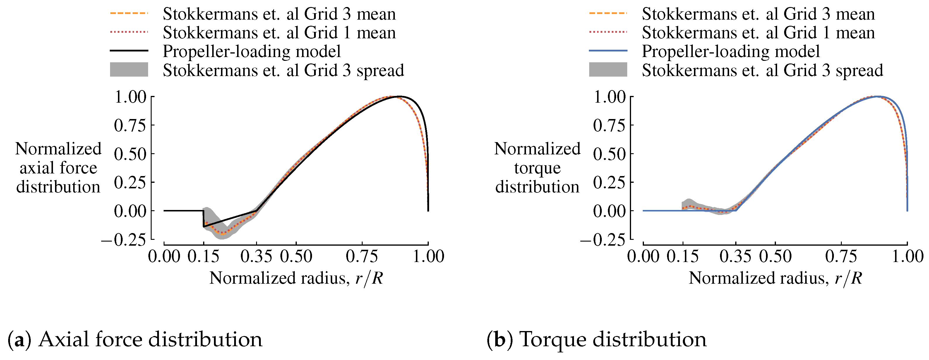
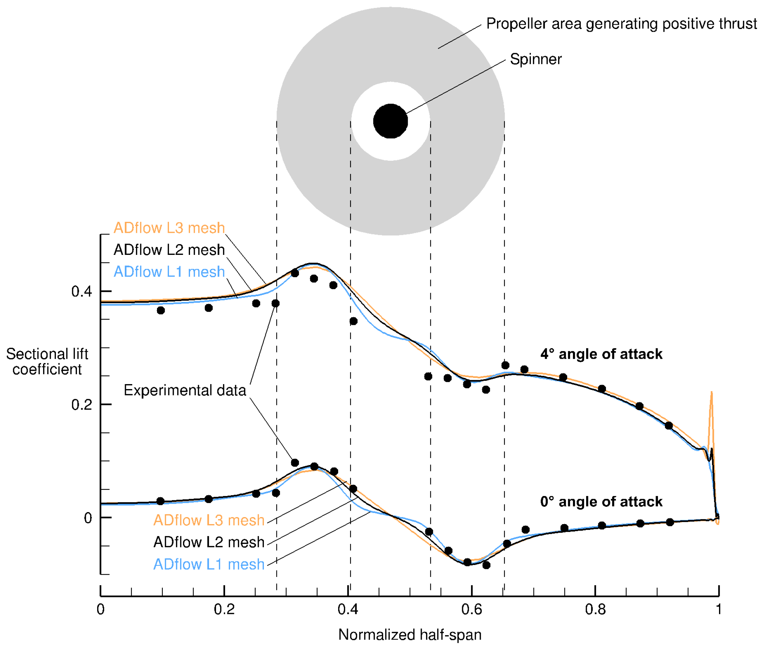
3.4. Validation Results

Sectional lift coefficients from ADflow and experimental data for the 0 ° and 4 ° validation cases are compared in Figure 7. The results match the experimental data well, with the 4 ° case having slightly more noticeable discrepancies. The pressure coefficient ( C p ) distributions of two wing sections behind the propeller are compared with experimental data in Figure 8 for the 4 ° case. The shapes match well, with some offsets. Numerous sources of error exist, including the absence of the nacelle in our simplified geometry and the axisymmetric propeller model’s inability to capture non-axisymmetric propeller loading due to propeller incidence and wing upwash. Figure A1 and Figure A2 in Appendix A show grid-convergence plots for the integrated lift coefficient C L and drag coefficient C D of the wing.

4. Optimization Problem Descriptions

4.1. Geometry and Parameterization

We use 10X-scaled versions of the wing and propeller geometry that were used for the validation cases for the optimization cases (i.e., a 2.4 m × 6.4 m half-wing with a 2.4 m diameter propeller). This scale is representative of the size of typical twin-propeller general-aviation (GA) and commuter-aircraft wings. We relocate the propeller in the spanwise direction such that its rotation axis is at the wingtip (i.e., 6.4 m from the root instead of 3 m from the root). We reuse the L2 propeller-region and wing surface meshes that were used for the validation cases by scaling them 10X. As shown by the validation results, the L2 meshes provide a good balance of resolution and computational cost. The wing volume mesh is re-generated with the thickness of the first off-wall layer set to a flat-plate y + value of 1 and with the maximum off-wall growth ratios of the layers ranging primarily between 1.2 and 1.3. Because the location of the propeller-region volume mesh is not the same as for the validation cases, we generate a new background mesh using the same approach that was used for the validation cases. These meshes are shown in Figure 9 and Figure 10.
We use the grid of FFD control points shown in Figure 11 to modify the geometry. The positions of these control points are the design variables. The grid has 11 sections along the span and 8 sections along the chord. There are 88 control points above the wing and 88 below it (176 in total). The control points of each section along the span can be rigidly rotated together to twist the wing, and all the control points can be moved individually in the vertical direction (y-direction) to change the airfoil shapes of the wing. The planform area and planform shape of the wing are not optimized in the cases presented in this paper. We place control points closer together for the portion of the wing behind the propeller disk for greater control. We optimize only the wing, and the optimizations begin with the wing being untwisted and with both the wing and the propeller at an angle of attack of 0 ° . The actuator disk keeps its inclination of 0 ° and does not follow the wing as the wing’s inclination changes.

4.2. Flight Conditions

We use flight conditions representative of a cruise condition for general aviation (GA) and urban air mobility (UAM). We specify a cruise C L of 0.6 at a Mach number of 0.3 and an altitude of 1500 ft. We assume that the hypothetical twin-propeller aircraft has a cruise lift-to-drag ratio of 10, and we set the propeller thrust equal to the half-aircraft drag based on these numbers (i.e., 5.5 kN, or C T = T / ( ρ ν 2 D 4 ) = 0.20 ). Assuming a rotational tip speed of Mach 0.6 (typical for turboprop aircraft at cruise), the corresponding advance ratio J is 1.6. This thrust coefficient is on the higher side of the range for typical GA and commuter aircraft at cruise [64,65,66]. Based on the efficiency charts of typical propellers [64,65,67], the pitch angle at 0.75  R for this advance ratio will likely be in the 35 ° to 40 ° range. Therefore, for the optimization cases, we use a P / D value of 1.7, which corresponds to a pitch angle of 36 ° . For the propeller-model shape parameter n, we use the same value used for the validation cases ( n = 0.2 ). These flight conditions and propeller settings are summarized in Table 2 and Table 3, respectively.

4.3. Optimization Problem Formulations

Table 4 summarizes the optimization problem formulation for the first optimization case: Case wP+T. In Case wP+T, we optimize the wing twist (T) with the propeller (wP) model included in the simulations during optimization. The twist is controlled by rigidly rotating the FFD control points of each of the 11 FFD sections along the span about their respective quarter-chord points. We optimize the wing twist using all 11 FFD sections, including the root section. Therefore, the twist design variables can also rotate the entire wing and effectively change its angle of attack without changing the angle of attack of the propeller disk. The optimization objective is to minimize C D , subject to a lift constraint of C L = 0.6 . These coefficients are only for the wing and are computed by integrating the forces on the wing surface. They do not include components of the propeller’s thrust vector, which remains at an inclination of 0 ° . These coefficients also do not include any contributions from other components of the hypothetical aircraft.
Table 5 summarizes the optimization problem formulation for the second optimization case: Case wP+T+S. In Case wP+T+S, we optimize the wing twist (T) and wing airfoil shapes (S) with the propeller (wP) model included in the simulations during optimization. The twist is controlled by rigidly rotating the FFD control points of each section, as described earlier, and the airfoil shapes along the wing are controlled by vertically displacing the individual FFD control points. The optimization objective is again to minimize C D , subject to a lift constraint of C L = 0.6 .
Because structural and internal-volume tradeoffs are not modeled in this work, we use thickness constraints to prevent the thickness of the wing from decreasing. The thickness constraints are set up by creating a uniformly spaced 2-D grid of points that lie within the wing and projecting them in the normal direction to the 2-D grid onto the upper and lower surfaces of a triangulated surface representation of the wing. The distances between the upper and lower projected points are used as the thicknesses. During optimization, these projected points are moved by the FFD control points in the same manner as the wing surface and are used to calculate the thicknesses for the new designs. For this work, we use a 10 × 10 grid to enforce these constraints.
Additionally, we apply constraints on the leading-edge and trailing-edge airfoil-shape design variables to prevent them from moving the leading and trailing edges vertically and from creating a shear twist. This is achieved by ensuring that the airfoil-shape design variables only move the FFD control points on the leading and trailing edges by equal distances in opposite directions within each vertical pair. By doing this, the twist and airfoil-shape design variables remain independent without restricting the optimizer’s ability to add camber, giving a well-posed optimization problem.

4.4. Baseline Optimization Cases for Comparison

For comparison, we also optimize the wing without accounting for propeller effects. The first baseline optimization case, Case T, has the same formulation as Case wP+T, except that no forces are applied to the actuator disk. The second baseline optimization case, Case T+S, has the same formulation as Case wP+T+S, except that no forces are applied to the actuator disk. The FFD grid used for these baseline cases is the same grid used for the wP cases (Figure 11). After optimization, the resulting wings from these baseline cases are re-simulated with the propeller forces applied to the actuator disk and the wing angle of attack adjusted to achieve the specified C L of 0.6. This angle-of-attack adjustment is performed using the FFD grid and the optimizer. This gives one-to-one comparisons that allow quantifying the benefit of optimizing a wing while accounting for propeller effects.

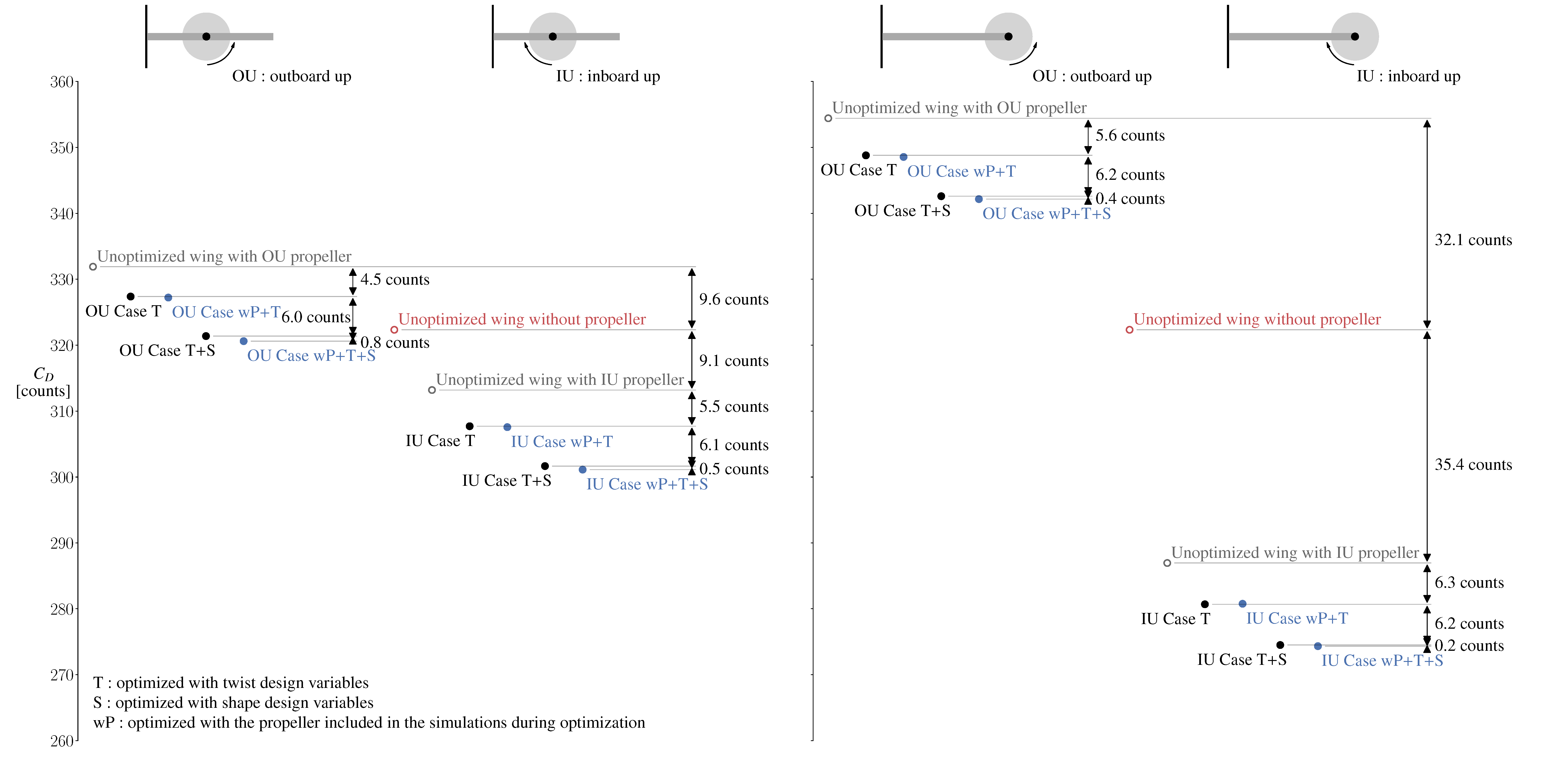
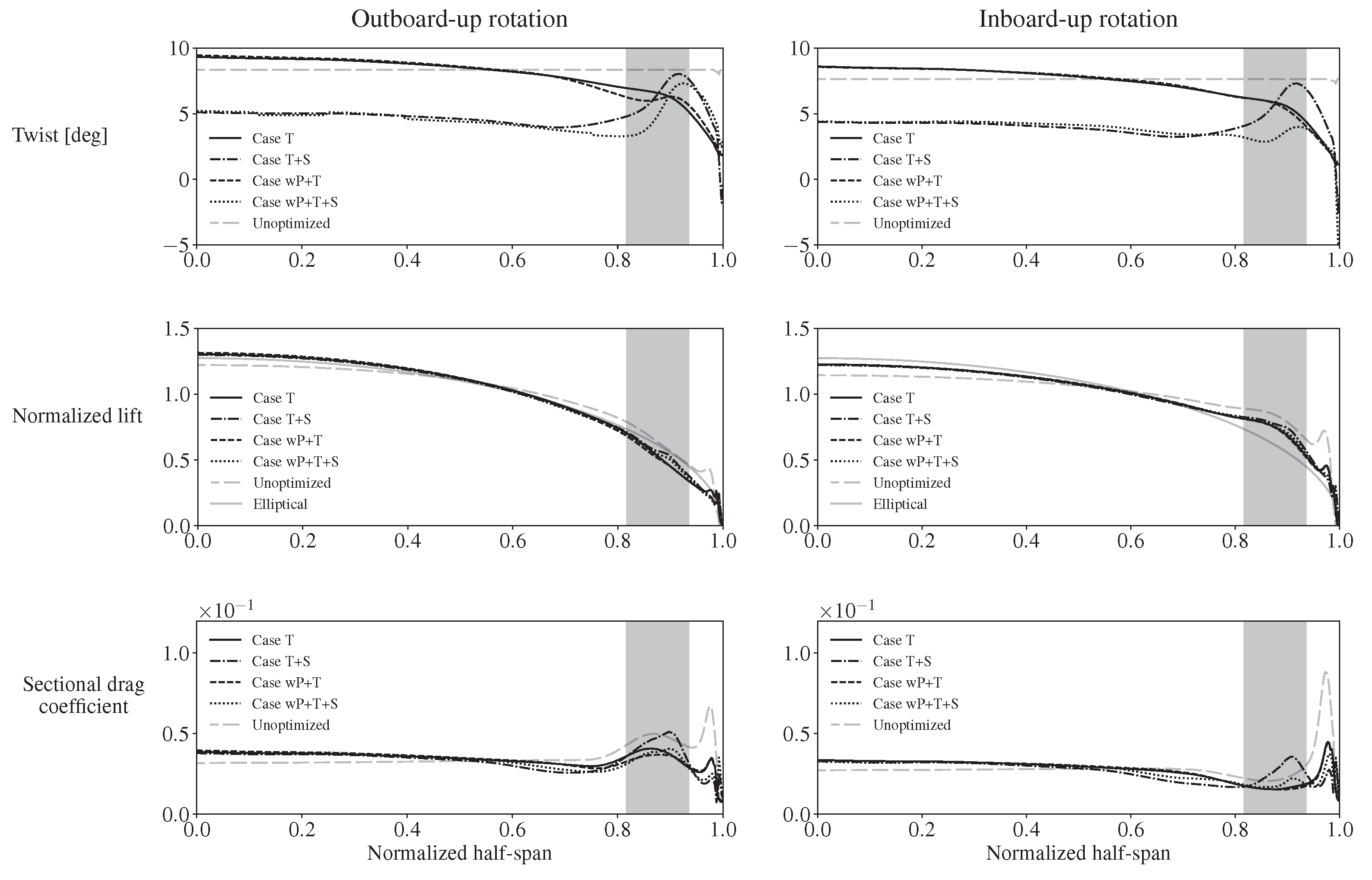
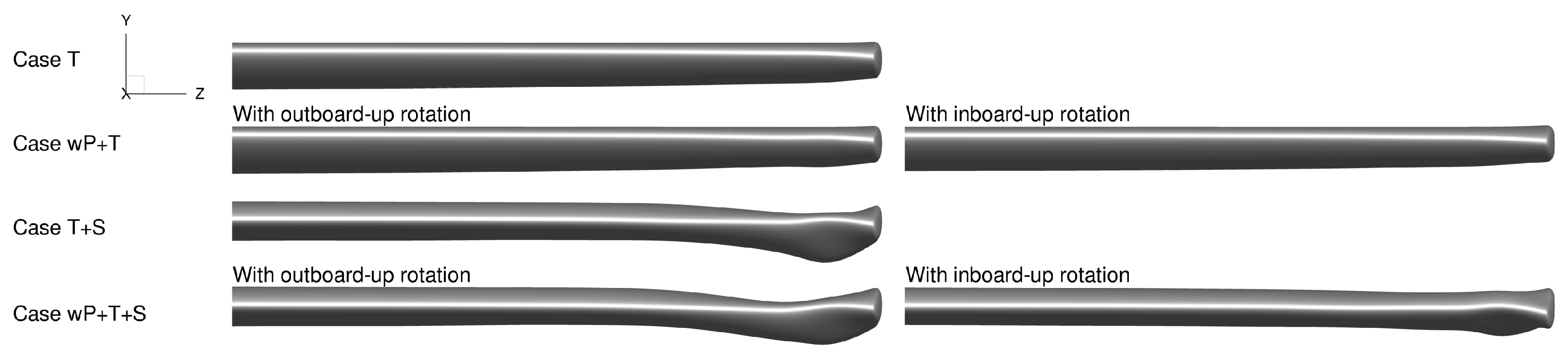
5. Optimization Results

The final drag coefficients from this work’s optimization cases, as well as from our previous work [17] for the same wing with an inboard propeller (same flight conditions, propeller settings, and optimization problem formulation but different propeller location), are plotted in Figure 12. Although the drag reductions from changing the propeller rotation direction from outboard-up to inboard-up (∼67 counts) and optimizing the wing twist and airfoil shapes (∼12 counts) are significant, the additional drag reductions obtained by optimizing the wing while accounting for the propeller slipstream during optimization are negligible (less than one drag count). This is the same conclusion we reached in previous work for a wing with an inboard propeller, despite the propeller slipstream’s significantly greater influence on the wing’s drag when located at the wingtip. The wings optimized without the propeller (Case T and Case T+S) are re-simulated with the propeller model after optimization, and the wing angle of attack is adjusted again using the optimizer to achieve the target C L of 0.6 for the final drag coefficients shown in Figure 12. Optimization convergence plots for the wing’s C L and C D are included in Appendix B.
When the propeller model is included in the simulations during optimization (Cases wP+T and wP+T+S), the optimizer decreases the twist angle behind the propeller for both the inboard-up and outboard-up cases, as shown in Figure 13. The twist distributions shown here are computed using the deformed wing surface and are not the twist parameter values of the FFD sections. There are also small related reductions in lift behind the propeller and increased lift inboard to compensate, as shown in Figure 13. When airfoil-shape design variables are added (Cases T+S and wP+T+S), the twist angles over most of the wing decrease because the optimizer adds camber. The nonplanar wingtips (Figure 14 and Figure 15) can be attributed to induced-drag reductions from a reduction in average wing downwash as the shed vorticity is moved away from the wing plane [68]. When the propeller’s rotation direction is the opposite of that of the wing-induced flow around the wingtip, we obtain a less-deformed wingtip (Figure 14 and Figure 15). The shapes and corresponding C p distributions for two wing sections directly behind the propeller (at 85 % b / 2 and 90 % b / 2 ) and for a wing section away from the propeller (at 50 % b / 2 ) are compared in Figure 16 and Figure 17. Nonplanar wingtips are obtained both with and without accounting for propeller effects. Similar nonplanar wingtips from twist optimization for wings without propellers were obtained by Bons et al. [69] and Reist et al. [70]. The designs presented here are not suitable for a production aircraft for multiple reasons, including the absence of nacelles. However, our goal in this study is to bracket the potential for drag reduction with twist and airfoil-shape design variables.
Figure 12. Reference and optimized drag coefficients show that the additional drag reductions obtained by optimizing the wing while accounting for the propeller slipstream during optimization are negligible. Results for an inboard-propeller configuration are included for reference [17] ( C L = 0.6 for all).
Aerospace 11 00512 g012
The lift distributions of the optimized wings are not elliptical (Figure 13), as expected [22]. From a lifting-line perspective, induced drag can be expressed as the span integral of the product of circulation, downwash, and density. Therefore, it is advantageous to have more lift (i.e., more circulation) behind the propeller when the propeller induces an upwash (i.e., negative downwash) and less lift behind the propeller when the propeller induces a downwash.
Figure 13 also shows that for each propeller rotation direction, the resulting lift distributions do not have significant differences when the wing is optimized while accounting for the propeller slipstream. The drag coefficient curves show that when the propeller model is included during optimization, the optimizer decreases the drag behind the propeller (for reference, breakdowns of the drag coefficient into pressure and shear components are shown in Figure A5 in Appendix C). However, there are also associated reductions in lift behind the propeller, and the adjustments required to satisfy the lift requirement cause these drag reductions to come with drag penalties inboard that reduce the overall benefit. This indicates that at least for similar configurations and operating conditions (i.e., low-sweep, low-taper, moderate-aspect-ratio wings with propeller diameter-to-wing-chord ratios, disk loadings, and operating conditions typical for twin-engined GA and commuter aircraft), a wing optimized without considering the propeller slipstream can recover swirl as effectively as a wing optimized while accounting for the propeller slipstream. Propeller-induced tangential velocities can be shown to be approximately proportional to disk loading and inversely proportional to tip speed and fluid density [62]. Additionally, from momentum theory, propeller-induced axial velocities are a function of the flight speed, fluid density, and disk loading. Therefore, this conclusion should be applicable to smaller and larger configurations that operate with similar disk loadings at flight conditions and tip Mach numbers typical for GA aircraft.

6. Conclusions

In this work, we implemented an actuator-disk propeller model in a CFD solver and performed RANS-based aerodynamic shape optimization studies for a wing with a propeller located in front of the wingtip using the open-source aerodynamics modules of the MACH framework. We solved eight optimization problems using gradient-based optimization enabled by efficient adjoint gradient computation. The objective is to minimize the drag for a cruise condition representative of GA and commuter operations using twist and airfoil-shape design variables.
The drag reductions from changing the propeller rotation direction from outboard-up to inboard-up (∼67 counts) and optimizing the wing twist and airfoil shapes (∼12 counts) are significant. However, the additional drag reductions obtained by optimizing the wing while accounting for the propeller slipstream are negligible (less than one drag count) when compared with optimizing the wing without accounting for the propeller and then simulating the optimized design with the propeller model and with the wing angle of attack adjusted to achieve the target C L .
The wings that were optimized without considering the propeller slipstream recover swirl as effectively as the ones optimized while accounting for the propeller slipstream. This means that it is not worthwhile to account for propeller–wing interaction while optimizing the wing twist and airfoil shapes to minimize cruise drag, at least for similar configurations and operating conditions (i.e., low-sweep, low-taper, moderate-aspect-ratio wings with propeller diameter-to-wing-chord ratios, disk loadings, and operating conditions typical for twin-engined GA and commuter aircraft).
The results show that it is more important to strategically select the propeller location and rotation direction. This is the same conclusion we reached in previous work for a wing with an inboard propeller, despite the propeller slipstream’s significantly greater influence on the wing’s drag when located at the wingtip.
A recommendation for future work is to couple a propeller-loading model, such as a blade-element model, to the CFD model in a manner that uses the flowfield from the CFD solution as the inflow for computing the propeller loading distributions. This will allow modeling changes in the performance of the propeller due to wing-design and propeller-inclination changes and also allow studying pusher-propeller configurations, for which the wing’s influence on the propeller due to induced velocities and blockage effects is more significant.

Author Contributions

Conceptualization, S.S.C. and J.R.R.A.M.; methodology, S.S.C. and J.R.R.A.M.; software, S.S.C.; validation, S.S.C.; investigation, S.S.C.; resources, J.R.R.A.M.; writing—original draft preparation, S.S.C.; writing—review and editing, S.S.C. and J.R.R.A.M.; visualization, S.S.C.; supervision, J.R.R.A.M.; project administration, J.R.R.A.M.; funding acquisition, J.R.R.A.M. All authors have read and agreed to the published version of the manuscript.

Funding

This research was funded by the Hyundai Motor Company.

Institutional Review Board Statement

Not applicable.

Informed Consent Statement

Not applicable.

Data Availability Statement

All publicly available data are within the manuscript.

Acknowledgments

The authors thank the Hyundai Motor Company for sponsoring this work. The authors also thank Charles Mader, Nicolas Bons, Anil Yildirim, Yingqian Liao, Eirikur Jonsson, Ella Wu, and Ping He for their helpful suggestions and invaluable support with the various computational tools used for this work. This research was also supported in part through computational resources and services provided by Advanced Research Computing at the University of Michigan, Ann Arbor.

Conflicts of Interest

The authors declare that this study received funding from the Hyundai Motor Company. The funder was not involved in the study design, collection, analysis, interpretation of data, the writing of this article, or the decision to submit this article for publication.

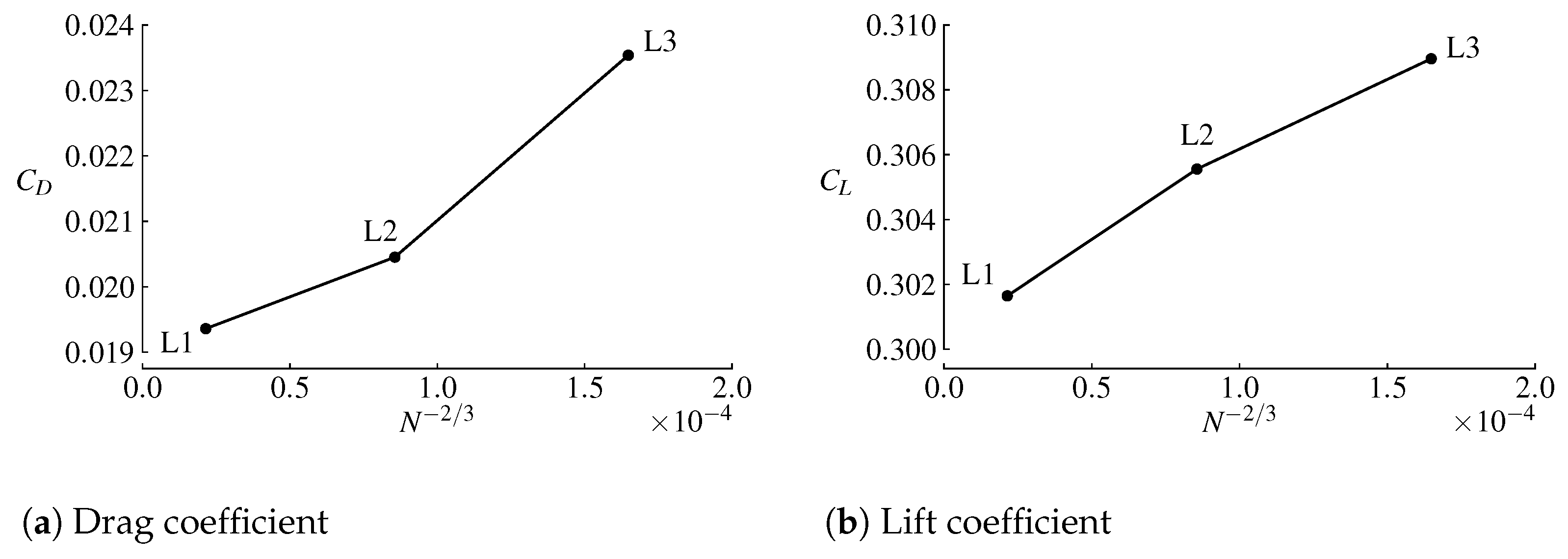
Appendix A. Mesh Refinement Study

Figure A1 and Figure A2 plot the C L and C D of the wing for the validation cases. The CFD solver settings and angle of attack are kept the same for all of the meshes within each of these cases. These coefficients are for only the wing and are computed by integrating the forces on the wing surface. We plot the coefficients with respect to N 2 / 3 , where N is the number of computation cells, because the inverse of the cube root of the number of cells gives a metric for the grid spacing and because ADflow uses a second-order-accurate finite-volume approach for the spatial discretization.
Figure A1. Mesh refinement plots for the 0 ° validation case (N is the number of computation cells).
Aerospace 11 00512 g0a1
Figure A2. Mesh refinement plots for the 4 ° validation case (N is the number of computation cells).
Aerospace 11 00512 g0a2

Appendix B. Optimization Convergence Plots

Figure A3 shows the C L and C D optimization convergence histories for Case wP+T and Case wP+T+S. The cases without airfoil shape design variables (Case wP+T) pose an easier optimization problem and require fewer iterations to converge.
Figure A4 shows the C L and C D optimization convergence histories for the second step for Case T and Case T+S. In this second step, the optimized wings are re-simulated with the propeller model, and the optimizer is again used to change the wing angle of attack to achieve the target C L of 0.6.
Figure A3. C L and C D optimization convergence histories for Case wP+T and Case wP+T+S.
Aerospace 11 00512 g0a3
Figure A4. C L and C D optimization convergence histories for the second step for Case T and Case T+S.
Aerospace 11 00512 g0a4

Appendix C. Spanwise Drag-Coefficient Breakdowns for Optimization Results

Figure A5 breaks down the optimized drag coefficient distributions into shear and pressure components. The propeller has a noticeably greater influence on the pressure drag than on the shear drag.
Figure A5. Optimized drag coefficient breakdowns for the primary and baseline optimization cases (the portion behind the propeller’s positive-thrust region is shaded).
Aerospace 11 00512 g0a5

References

  1. Moore, M.D.; Fredericks, B. Misconceptions of Electric Aircraft and their Emerging Aviation Markets. In Proceedings of the 52nd Aerospace Sciences Meeting, National Harbor, MD, USA, 13–17 January 2014; Number AIAA 2014-0534. AIAA: Reston, VA, USA, 2014; p. 2014-0535. [Google Scholar] [CrossRef]
  2. Patterson, M.D.; German, B. Conceptual Design of Electric Aircraft with Distributed Propellers: Multidisciplinary Analysis Needs and Aerodynamic Modeling Development. In Proceedings of the 52nd Aerospace Sciences Meeting, National Harbor, MD, USA, 13–17 January 2014; Number AIAA 2014-0534. AIAA: Reston, VA, USA, 2014. [Google Scholar] [CrossRef]
  3. Stoll, A.M.; Bevirt, J.; Moore, M.D.; Fredericks, W.J.; Borer, N.K. Drag Reduction Through Distributed Electric Propulsion. In Proceedings of the 14th AIAA Aviation Technology, Integration, and Operations Conference, Atlanta, GA, USA, 16–20 June 2014; Number AIAA 2014-2851. AIAA: Reston, VA, USA, 2014. [Google Scholar] [CrossRef]
  4. Stoll, A.M.; Bevirt, J.; Pei, P.P.; Stilson, E.V. Conceptual Design of the Joby S2 Electric VTOL PAV. In Proceedings of the 14th AIAA Aviation Technology, Integration, and Operations Conference, Atlanta, GA, USA, 16–20 June 2014; Number AIAA 2014-2407. AIAA: Reston, VA, USA, 2014. [Google Scholar] [CrossRef]
  5. Duffy, M.J.; Wakayama, S.R.; Hupp, R.; Lacy, R.; Stauffer, M. A Study in Reducing the Cost of Vertical Flight with Electric Propulsion. In Proceedings of the 17th AIAA Aviation Technology, Integration, and Operations Conference, Denver, CO, USA, 5–9 June 2017; Number AIAA 2017-3442. AIAA: Reston, VA, USA, 2017. [Google Scholar] [CrossRef]
  6. Deere, K.A.; Viken, S.A.; Carter, M.B.; Viken, J.K.; Derlaga, J.M.; Stoll, A.M. Comparison of High-Fidelity Computational Tools for Wing Design of a Distributed Electric Propulsion Aircraft. In Proceedings of the 35th AIAA Applied Aerodynamics Conference, Denver, CO, USA, 5–9 June 2017; Number AIAA 2017-3925. AIAA: Reston, VA, USA, 2017. [Google Scholar] [CrossRef]
  7. Fredericks, W.J.; McSwain, R.G.; Beaton, B.F.; Klassman, D.W.; Theodore, C.R. Greased Lightning (GL-10) Flight Testing Campaign; Technical Memorandum NASA-TM-2017-219643; NASA: Washington, DC, USA, 2017. [Google Scholar]
  8. Antcliff, K.R.; Capristan, F.M. Conceptual Design of the Parallel Electric-Gas Architecture with Synergistic Utilization Scheme (PEGASUS) Concept. In Proceedings of the 18th AIAA/ISSMO Multidisciplinary Analysis and Optimization Conference, Denver, CO, USA, 5–9 June 2017; Number AIAA 2017-4001. AIAA: Reston, VA, USA, 2017. [Google Scholar] [CrossRef]
  9. Alba, C.; Elham, A.; German, B.J.; Veldhuis, L.L.M. A surrogate-based multi-disciplinary design optimization framework modeling wing-propeller interaction. Aerosp. Sci. Technol. 2018, 78, 721–733. [Google Scholar] [CrossRef]
  10. Hwang, J.T.; Ning, A. Large-scale multidisciplinary optimization of an electric aircraft for on-demand mobility. In Proceedings of the 2018 AIAA/ASCE/AHS/ASC Structures, Structural Dynamics, and Materials Conference, Kissimmee, FL, USA, 8–12 January 2018; Number AIAA 2018-1384. AIAA: Reston, VA, USA, 2018. [Google Scholar] [CrossRef]
  11. Droandi, G.; Syal, M.; Bower, G. Tiltwing Multi-Rotor Aerodynamic Modeling in Hover, Transition and Cruise Flight Conditions. In Proceedings of the AHS International Forum 74, Phoenix, AZ, USA, 14–17 May 2018; Paper 74-2018-1267. VFS: Fairfax, VA, USA, 2018. [Google Scholar]
  12. Brelje, B.J.; Martins, J.R.R.A. Electric, Hybrid, and Turboelectric Fixed-Wing Aircraft: A Review of Concepts, Models, and Design Approaches. Prog. Aerosp. Sci. 2019, 104, 1–19. [Google Scholar] [CrossRef]
  13. Moore, K.R.; Ning, A. Takeoff and Performance Trade-Offs of Retrofit Distributed Electric Propulsion for Urban Transport. J. Aircr. 2019, 56, 1880–1892. [Google Scholar] [CrossRef]
  14. De Vries, R.; Brown, M.; Vos, R. Preliminary Sizing Method for Hybrid-Electric Distributed-Propulsion Aircraft. J. Aircr. 2019, 56, 2172–2188. [Google Scholar] [CrossRef]
  15. Chauhan, S.S.; Martins, J.R.R.A. Tilt-Wing eVTOL Takeoff Trajectory Optimization. J. Aircr. 2020, 57, 93–112. [Google Scholar] [CrossRef]
  16. Hoogreef, M.; de Vries, R.; Sinnige, T.; Vos, R. Synthesis of Aero-Propulsive Interaction Studies Applied to Conceptual Hybrid-Electric Aircraft Design. In Proceedings of the AIAA Scitech 2020 Forum, Orlando, FL, USA, 6–10 January 2020; Number AIAA 2020-0503. AIAA: Reston, VA, USA, 2020. [Google Scholar] [CrossRef]
  17. Chauhan, S.S.; Martins, J.R.R.A. RANS-Based Aerodynamic Shape Optimization of a Wing Considering Propeller-Wing Interaction. J. Aircr. 2021, 58, 497–513. [Google Scholar] [CrossRef]
  18. Prandtl, L. Mutual Influence of Wings and Propeller; Technical Note NACA-TN-74, NACA; An English translation of an extract from the First Report of the Göttingen Aerodynamic Laboratory; NACA: Hampton, VA, USA, 1921. [Google Scholar]
  19. Kuhn, R.E.; Draper, J.W. An Investigation of a Wing-Propeller Configuration Employing Large-Chord Plain Flaps and Large-Diameter Propellers for Low-Speed Flight and Vertical Take-Off; Technical Note NACA-TN-3307; NACA: Hampton, VA, USA, 1954. [Google Scholar]
  20. Kuhn, R.E.; Draper, J.W. Investigation of the Aerodynamic Characteristics of a Model Wing-Propeller Combination and of the Wing and Propeller Separately at Angles of Attack up to 90°; Technical Report NACA-TR-1263; NACA: Hampton, VA, USA, 1956. [Google Scholar]
  21. Snyder, M.H., Jr.; Zumwalt, G.W. Effects of Wingtip-Mounted Propellers on Wing Lift and Induced Drag. J. Aircr. 1969, 6, 392–397. [Google Scholar] [CrossRef]
  22. Kroo, I. Propeller-Wing Integration For Minimum Induced Loss. J. Aircr. 1986, 23, 561–565. [Google Scholar] [CrossRef]
  23. Miranda, L.R.; Brennan, J.E. Aerodynamic Effects of Eingtip-Mounted Propellers and Turbines. In Proceedings of the 4th Applied Aerodynamics Conference, San Diego, CA, USA, 9–11 June 1986; Number AIAA 1986-1802. AIAA: Reston, VA, USA, 1986. [Google Scholar] [CrossRef]
  24. Veldhuis, L.L.M. Propeller Wing Aerodynamic Interference. Ph.D Thesis, Delft University of Technology, Delft, The Netherlands, 2005. [Google Scholar]
  25. Sinnige, T.; van Arnhem, N.; Stokkermans, T.C.A.; Eitelberg, G.; Veldhuis, L.L.M. Wingtip-Mounted Propellers: Aerodynamic Analysis of Interaction Effects and Comparison with Conventional Layout. J. Aircr. 2019, 56, 295–312. [Google Scholar] [CrossRef]
  26. Miley, S.J.; Howard, R.M.; Holmes, B.J. Wing Laminar Boundary Layer in the Presence of a Propeller Slipstream. J. Aircr. 1988, 25, 606–611. [Google Scholar] [CrossRef]
  27. Stokkermans, T.; Veldhuis, L.; Soemarwoto, B.; Fukari, R.; Eglin, P. Breakdown of aerodynamic interactions for the lateral rotors on a compound helicopter. Aerosp. Sci. Technol. 2020, 101, 105845. [Google Scholar] [CrossRef]
  28. Whitfield, D.L.; Jameson, A. Euler Equation Simulation of Propeller-Wing Interaction in Transonic Flow. J. Aircr. 1984, 21, 835–839. [Google Scholar] [CrossRef]
  29. Witkowski, D.P.; Lee, A.K.H.; Sullivan, J.P. Aerodynamic Interaction Between Propellers and Wings. J. Aircr. 1989, 26, 829–836. [Google Scholar] [CrossRef]
  30. Ardito Marretta, R.M.; Davi, G.; Milazzo, A.; Lombardi, G. Wing Pitching and Loading with Propeller Interference. J. Aircr. 1999, 36, 468–471. [Google Scholar] [CrossRef]
  31. Veldhuis, L.L.M.; Heyma, P.M. Aerodynamic optimisation of wings in multi-engined tractor propeller arrangements. Aircr. Des. 2000, 3, 129–149. [Google Scholar] [CrossRef]
  32. Moens, F.; Gardarein, P. Numerical Simulation of the Propeller/Wing Interactions for Transport Aircraft. In Proceedings of the 19th AIAA Applied Aerodynamics Conference, Anaheim, CA, USA, 11–14 June 2001; Number AIAA 2001-2404. AIAA: Reston, VA, USA, 2001. [Google Scholar] [CrossRef]
  33. Roosenboom, E.W.M.; Stürmer, A.; Schröder, A. Advanced Experimental and Numerical Validation and Analysis of Propeller Slipstream Flows. J. Aircr. 2010, 47, 284–291. [Google Scholar] [CrossRef]
  34. Gomariz-Sancha, A.; Maina, M.; Peace, A.J. Analysis of propeller-airframe interaction effects through a combined numerical simulation and wind-tunnel testing approach. In Proceedings of the 53rd AIAA Aerospace Sciences Meeting, Kissimmee, FL, USA, 5–9 January 2015; Number AIAA 2015-1026. AIAA: Reston, VA, USA, 2015. [Google Scholar] [CrossRef]
  35. Rakshith, B.R.; Deshpande, S.M.; Narasimha, R.; Praveen, C. Optimal Low-Drag Wing Planforms for Tractor-Configuration Propeller-Driven Aircraft. J. Aircr. 2015, 52, 1791–1801. [Google Scholar] [CrossRef]
  36. Epema, K. Wing Optimisation for Tractor Propeller Configurations. Master’s Thesis, Delft University of Technology, Delft, The Netherlands, 2017. [Google Scholar]
  37. Stokkermans, T.C.A.; van Arnhem, N.; Sinnige, T.; Veldhuis, L.L.M. Validation and Comparison of RANS Propeller Modeling Methods for Tip-Mounted Applications. AIAA J. 2019, 57, 566–580. [Google Scholar] [CrossRef]
  38. Van Arnhem, N.; de Vries, R.; Sinnige, T.; Vos, R.; Veldhuis, L.L.M. Aerodynamic Performance and Static Stability Characteristics of Aircraft with Tail-Mounted Propellers. J. Aircr. 2022, 59, 415–432. [Google Scholar] [CrossRef]
  39. Koyuncuoglu, H.U.; He, P. Simultaneous wing shape and actuator parameter optimization using the adjoint method. Aerosp. Sci. Technol. 2022, 130, 107876. [Google Scholar] [CrossRef]
  40. Russo, O.; Aprovitola, A.; de Rosa, D.; Pezzella, G.; Viviani, A. Computational Fluid Dynamics Analyses of a Wing with Distributed Electric Propulsion. Aerospace 2023, 10, 64. [Google Scholar] [CrossRef]
  41. Alvarez, E.J.; Ning, A. Meshless Large-Eddy Simulation of Propeller–Wing Interactions with Reformulated Vortex Particle Method. J. Aircr. 2024, 61. [Google Scholar] [CrossRef]
  42. Pedreiro, L.N. Estudo e otimização de uma asa sob efeito de hélice na configuração tractor para redução de arrasto. Master’s Thesis, Universidade Federal de Minas Gerais, Belo Horizonte, MG, Brazil, 2017. [Google Scholar]
  43. Martins, J.R.R.A. Aerodynamic Design Optimization: Challenges and Perspectives. Comput. Fluids 2022, 239, 105391. [Google Scholar] [CrossRef]
  44. Yildirim, A.; Kenway, G.K.W.; Mader, C.A.; Martins, J.R.R.A. A Jacobian-free approximate Newton–Krylov startup strategy for RANS simulations. J. Comput. Phys. 2019, 397, 108741. [Google Scholar] [CrossRef]
  45. Mader, C.A.; Kenway, G.K.W.; Yildirim, A.; Martins, J.R.R.A. ADflow: An Open-Source Computational Fluid Dynamics Solver for Aerodynamic and Multidisciplinary Optimization. J. Aerosp. Inf. Syst. 2020, 17, 508–527. [Google Scholar] [CrossRef]
  46. Lee, Y.; Baeder, J. Implicit hole cutting—A new approach to overset grid connectivity. In Proceedings of the 16th AIAA Computational Fluid Dynamics Conference, Orlando, FL, USA, 23–26 June 2003; Number AIAA 2003-4128. AIAA: Reston, VA, USA, 2003. [Google Scholar] [CrossRef]
  47. Landmann, B.; Montagnac, M. A highly automated parallel Chimera method for overset grids based on the implicit hole cutting technique. Int. J. Numer. Methods Fluids 2011, 66, 778–804. [Google Scholar] [CrossRef]
  48. Kenway, G.K.W.; Secco, N.; Martins, J.R.R.A.; Mishra, A.; Duraisamy, K. An Efficient Parallel Overset Method for Aerodynamic Shape Optimization. In Proceedings of the 58th AIAA/ASCE/AHS/ASC Structures, Structural Dynamics, and Materials Conference, AIAA SciTech Forum, Grapevine, TX, USA, 9–13 January 2017; Number AIAA 2017-0357. AIAA: Reston, VA, USA, 2017. [Google Scholar] [CrossRef]
  49. Jameson, A.; Schmidt, W.; Turkel, E. Numerical Solution of the Euler Equations by Finite Volume Methods Using Runge–Kutta Time Stepping Schemes. In Proceedings of the 14th Fluid and Plasma Dynamics Conference, Palo Alto, CA, USA, 23–25 June 1981; Number AIAA 1981-1259. AIAA: Reston, VA, USA, 1981. [Google Scholar] [CrossRef]
  50. Spalart, P.; Allmaras, S. A One-Equation Turbulence Model for Aerodynamic Flows. In Proceedings of the 30th Aerospace Sciences Meeting and Exhibit, Reno, NV, USA, 6–9 January 1992; Number AIAA 1992-439. AIAA: Reston, VA, USA, 1992. [Google Scholar] [CrossRef]
  51. Kenway, G.K.W.; Mader, C.A.; He, P.; Martins, J.R.R.A. Effective Adjoint Approaches for Computational Fluid Dynamics. Prog. Aerosp. Sci. 2019, 110, 100542. [Google Scholar] [CrossRef]
  52. Secco, N.; Kenway, G.K.W.; He, P.; Mader, C.A.; Martins, J.R.R.A. Efficient Mesh Generation and Deformation for Aerodynamic Shape Optimization. AIAA J. 2021, 59, 1151–1168. [Google Scholar] [CrossRef]
  53. Hascoët, L. TAPENADE: A tool for Automatic Differentiation of programs. In Proceedings of the 4th European Congress on Computational Methods, ECCOMAS’2004, Jyvaskyla, Finland, 24–28 July 2004. [Google Scholar]
  54. Hascoët, L.; Pascual, V. The Tapenade automatic differentiation tool: Principles, model, and specification. Acm Trans. Math. Softw. 2013, 39, 1–43. [Google Scholar] [CrossRef]
  55. Kenway, G.K.W.; Kennedy, G.J.; Martins, J.R.R.A. A CAD-Free Approach to High-Fidelity Aerostructural Optimization. In Proceedings of the 13th AIAA/ISSMO Multidisciplinary Analysis Optimization Conference, Fort Worth, TX, USA, 13–15 September 2010; Number AIAA 2010-9231. AIAA: Reston, VA, USA, 2010. [Google Scholar] [CrossRef]
  56. Luke, E.; Collins, E.; Blades, E. A Fast Mesh Deformation Method Using Explicit Interpolation. J. Comput. Phys. 2012, 231, 586–601. [Google Scholar] [CrossRef]
  57. Gill, P.E.; Murray, W.; Saunders, M.A. SNOPT: An SQP Algorithm for Large-Scale Constrained Optimization. Siam Rev. 2005, 47, 99–131. [Google Scholar] [CrossRef]
  58. Osusky, L.; Buckley, H.; Reist, T.; Zingg, D.W. Drag Minimization Based on the Navier–Stokes Equations Using a Newton–Krylov Approach. AIAA J. 2015, 53, 1555–1577. [Google Scholar] [CrossRef]
  59. Perez, R.E.; Jansen, P.W.; Martins, J.R.R.A. pyOpt: A Python-Based Object-Oriented Framework for Nonlinear Constrained Optimization. Struct. Multidiscip. Optim. 2012, 45, 101–118. [Google Scholar] [CrossRef]
  60. Wu, N.; Kenway, G.; Mader, C.A.; Jasa, J.; Martins, J.R.R.A. pyOptSparse: A Python framework for large-scale constrained nonlinear optimization of sparse systems. J. Open Source Softw. 2020, 5, 2564. [Google Scholar] [CrossRef]
  61. Hoekstra, M. A RANS-based analysis tool for ducted propeller systems in open water condition. Int. Shipbuild. Prog. 2006, 53, 205–227. [Google Scholar]
  62. Chauhan, S.S. Estimating propeller-induced tangential velocities by hand. 2023. preprint. Available online: http://doi.org/10.13140/RG.2.2.26021.88801 (accessed on 1 January 2024).
  63. Sinnige, T.; de Vries, R.; Corte, B.D.; Avallone, F.; Ragni, D.; Eitelberg, G.; Veldhuis, L.L.M. Unsteady Pylon Loading Caused by Propeller-Slipstream Impingement for Tip-Mounted Propellers. J. Aircr. 2018, 55, 1605–1618. [Google Scholar] [CrossRef]
  64. Biermann, D.; Hartman, E.P. Full-Scale Tests of 4- and 6-Blade, Single- and Dual-Rotating Propellers; Special Report NACA-SR-157; NACA: Hampton, VA, USA, 1940. [Google Scholar]
  65. Anonymous. Generalized Method of Propeller Performance Estimation; Technical Report PDB 6101 Revision A; Hamilton Standard: Windsor Locks, CT, USA, 1963. [Google Scholar]
  66. Raymer, D.P. Aircraft Design: A Conceptual Approach, 5th ed.; AIAA: Reston, VA, USA, 2012. [Google Scholar]
  67. McCormick, B.W. Aerodynamics of V/STOL Flight, 1st ed.; Academic Press: San Diego, CA, USA, 1967. [Google Scholar]
  68. Kroo, I.M. Drag due to Lift: Concepts for Prediction and Reduction. Annu. Rev. Fluid Mech. 2000, 33, 587–617. [Google Scholar] [CrossRef]
  69. Bons, N.P.; He, X.; Mader, C.A.; Martins, J.R.R.A. Multimodality in Aerodynamic Wing Design Optimization. AIAA J. 2019, 57, 1004–1018. [Google Scholar] [CrossRef]
  70. Reist, T.A.; Koo, D.; Zingg, D.W.; Bochud, P.; Castonguay, P.; Leblond, D. Cross Validation of Aerodynamic Shape Optimization Methodologies for Aircraft Wing-Body Optimization. AIAA J. 2020, 58. [Google Scholar] [CrossRef]
Figure 1. Geometry of the experimental configuration used for validation (half-wing planform area is 0.15 m2; aspect ratio is 5.3; reproduced with permission from Veldhuis [24]).
Aerospace 11 00512 g001
Figure 2. Surfaces and volume meshes.
Aerospace 11 00512 g002
Figure 3. Overset meshes.
Aerospace 11 00512 g003
Figure 4. Comparing L1, L2, and L3 grids.
Aerospace 11 00512 g004
Figure 5. Distributions of the axial and tangential forces from the propeller-loading model for the validation cases ( J = 0.85 and T C = 0.168 ).
Aerospace 11 00512 g005
Figure 6. The propeller-loading model compared with unsteady CFD results from Stokkermans et al. [37] (Grid 3 has 7.4 · 10 6 cells, and Grid 1 has 21.4 · 10 6 cells).
Aerospace 11 00512 g006
Figure 7. Sectional lift coefficients from ADflow compared with experimental data from Veldhuis [24].
Aerospace 11 00512 g007
Figure 8. Airfoil C p distributions from ADflow compared with experimental data from Veldhuis [24] for the 4 ° validation case (b is the wingspan, c is the chord length, and x and y are spatial coordinates).
Aerospace 11 00512 g008
Figure 9. Surfaces and volume meshes for the wingtip-propeller cases.
Aerospace 11 00512 g009
Figure 10. Overset meshes for the optimization cases.
Aerospace 11 00512 g010
Figure 11. FFD grid ( 8 × 2 × 11 control points) around the wing.
Aerospace 11 00512 g011
Figure 13. Optimized twist, lift, and drag distributions for the primary and baseline optimization cases (the portion behind the propeller’s positive-thrust region is shaded).
Aerospace 11 00512 g013
Figure 14. Front view of the optimized wings.
Aerospace 11 00512 g014
Figure 15. Rear view of the optimized wings.
Aerospace 11 00512 g015
Figure 16. Optimized wing C p distributions for outboard-up propeller rotation.
Aerospace 11 00512 g016
Figure 17. Optimized wing C p distributions for inboard-up propeller rotation.
Aerospace 11 00512 g017
Table 1. Total numbers of cells in the overset meshes.
MeshTotal Number of CellsTotal Number of Computation Cells, N
L110,621,44010,085,277
L21,343,5201,263,010
L3509,152472,605
Table 2. Flight conditions and aircraft specifications.
C L Mach NumberAltitudeAssumed Aircraft Lift-to-Drag RatioPropeller Tip Mach Number
0.60.31500 ft100.6
Table 3. Propeller specifications and nondimensional parameters.
Advance Ratio, V / ( ν D ) Thrust Coefficient, T / ( ρ ν 2 D 4 ) Thrust, TPitch-to-Diameter Ratio, P / D
1.60.205.5 kN1.7
Table 4. Case wP+T optimization problem formulation.
Function or VariableDescriptionQuantity
Minimize C D Drag coefficient
by varying  0 τ 10.0 Twist of each FFD section [ ° ]11
Total design variables11
subject to C L = 0.6 Lift constraint1
Total constraint functions1
Table 5. Case wP+T+S optimization problem formulation.
Function or VariableDescriptionQuantity
Minimize C D Drag coefficient
by varying 0 τ 10.0 Twist of each FFD section [ ° ]11
14.4 Δ y 14.4 Vertical displacements of the FFD control points for airfoil-shape
control ( ± 40 % of the airfoil maximum thickness) [cm]176
Total design variables187
subject to C L = 0.6 Lift constraint1
t a / t a , initial 1.0 Constraints to prevent airfoil thicknesses at locations on a uniform
10 × 10 grid from decreasing100
Δ y LE , upper = Δ y LE , lower Constraints to prevent the airfoil-shape design variables from
vertically displacing the leading edge11
Δ y TE , upper = Δ y TE , lower Constraints to prevent the airfoil-shape design variables from
vertically displacing the trailing edge11
Total constraint functions123
Disclaimer/Publisher’s Note: The statements, opinions and data contained in all publications are solely those of the individual author(s) and contributor(s) and not of MDPI and/or the editor(s). MDPI and/or the editor(s) disclaim responsibility for any injury to people or property resulting from any ideas, methods, instructions or products referred to in the content.

