1. Introduction
Many systems in the aviation industry work synchronously and need to be constructed after very detailed studies. One of these systems is the fuel system, which consists of many subsystems, such as storage, distribution, and indication [
1]. The fuel system of an airplane is a complex and crucial component that serves multiple purposes to guarantee the aircraft’s reliability, safety, and desired performance [
2,
3]. The storage system has limitations based on defined aircraft specifications, requiring an adjustment of tank geometry [
4]. Training aircraft fuel tanks have various custom geometries based on international aviation restrictions and requirements. The covering of the airframe to create a fuel tank is the limitation that determines this geometry [
5]. Thus, every tank geometry should be designed with detailed studies under this custom geometry [
6]. Constructing a fuel tank geometry in a volume that meets the fuel needs and related requirements is the first step in designing a fuel tank [
7].
A sufficient amount of fuel is required for predefined missions of training aircraft. Depending on the weight of aircraft and the required mission range, the necessary amount of fuel must be stored in aircraft tanks [
8]. Specifically, to increase an aircraft’s range, an additional fuel tank is mounted on both the fuselage and the wing structure [
9]. In addition, fuselage and wing tanks can be used as external tanks, and even vertical stabilizers can be used as fuel tanks. However, for the clean configuration of training aircraft, only wing tanks are considered, instead of fuselage, conformal, and external tanks [
10]. Wing tanks play a critical role in providing sufficient fuel to the engine. However, an excessive amount of fuel causes some problems in proportion to its mass [
11]. ‘Sloshing’ is the term used to describe unsteady movement of fuel within a tank, which significantly impacts flight mechanics during a mission. Due to this impact, wing tank geometry and fuel mass must be considered for aircraft stability [
12]. The CG deviation and retreat time are considered primary targets for evaluation to examine the effects of sloshing on stability. Deviation of CG is a situation caused by fluid flow in a fuel tank [
13]. During flight missions, aircraft perform various maneuvers. As a result of these maneuvers, external forces are applied to the aircraft structure, and these maneuvers also affect fluids in the fuel tank in terms of acceleration [
14]. Fluid movement occurs due to the accelerations acting on the fluid. Consequently, fuel motion in the wing tank of an aircraft leads to strict engineering problems [
15].
Depending on the volume fraction of fuel, it is assumed that there are two fluid phases in the fuel tank. Sloshing is the term for multiphase flow that occurs in a control volume [
16]. Measurements can be made to evaluate the sloshing effect on flight mechanics by establishing experimental test setups. Both commercial and military aircraft use these test rigs designed for sloshing [
17]. Test studies can give specific results for relevant tank geometry under certain external effects. Furthermore, the effects of this fluid flow can also be calculated using numerical analysis [
18]. Numerical calculations for sloshing analysis in a specific tank geometry give results parallel to experimental results. Considering the cost and measurement time, numerical calculations are preferred to observe the sloshing effects of the fuel tank [
19]. The aircraft’s flight mechanics and stability controls are evaluated based on CG deviation with 1D simulations and CFD calculations.
Deviations in an aircraft’s center of gravity can be managed thanks to the internal design of a wing fuel tank. Baffles are commonly used in wing fuel tanks to improve the structure further [
20]. The prominent role of baffles is to dampen sloshing effects with the help of cutout holes on them. Damping of sloshing phenomena is a solution to prevent aircraft from undergoing unsteady flight conditions caused by CG instabilities [
21]. Different baffle designs in the wing fuel tank compose various solutions to damp sloshing effects. The interior volume and baffle structures designed for wing fuel tanks in a training aircraft depend on many parameters. With these parameters, fuel tanks can be designed to absorb fuel-sloshing effects at different performances and contain enough fuel to meet aviation requirements. When analyses are performed for each design proposal of the fuel tank, the resulting amount will be numerous and examined one by one.
Managing vast amounts of data is a new challenge, as the number of outputs and inputs increases. The manual examination of each analysis to establish a logic between inputs and outputs becomes nearly impossible. However, this challenge can be overcome by connecting inputs and outputs with an artificial neural network. A sufficient number of analysis results are required for the learning algorithm of the ANN structure. Constructing a logic with an ANN opens the door to new and improved design proposals. Various types of ANN can be set up to process many results [
22]. In studies with artificial neural networks, a logical bound can be established between the program input parameters and the outputs [
23]. This logical bound between input parameters and outputs empowers the neural network to make predictions [
24]. The outputs obtained from 1D simulation data can be used as data to be taught for these neural networks. Thus, existing simulation outputs provide an input source for the ANN algorithm [
25].
In the current study, a novel and original method was developed for the evaluation of tank baffle design through numerous 1D analyses integrated with ANN to highlight the dominant parameters for further investigations with CFD analyses. Ultimately, it is vital to identify the parameters that affect fuel sloshing in a wing tank. When processed by ANN, the simulation results can identify the most influential parameters, enhancing the understanding of fuel tank dynamics.
The study is organized as follows. In the first part, a literature survey is written to highlight the novelty and originality of the current study. In the second part, the problem definition is given along with the geometric details of the baffles. The methodology section outlines the road map and engineering methods to be employed, detailing numerical explanations. The results section categorizes and details the numerical outputs obtained from 1D and 3D analyses and provides comments on selected cases based on parameter changes. Finally, in the conclusion section, the benefits and innovations of the study on the subject are summarized.
2. Problem Definition
While an aircraft is in the cruise flight condition, there is no acceleration acting on the aircraft. However, when an aircraft performs any maneuver, acceleration suddenly affects the entire aircraft’s body. However, fuel does not move immediately like the rigid body of an aircraft because of the fluid behavior of a partially filled fuel tank. Then, due to the inertial effects of the partially filled tank, a difference occurs between initial and transient CG location of the aircraft body. That difference is called CG deviation. When acceleration ends, and the aircraft returns to cruise flight conditions, the CG location will attempt to retreat from the momentary deviated location to its initial location. The time it takes for the CG value to return is called the retreat time. Depending on aerospace requirements, it is acceptable for CG locations to retreat to a point defined as a certain distance away from its initial location. The main goal of this study is to achieve the lowest CG deviation and the shortest retreat time values with the aid of 1D simulations, CFD calculations, and artificial intelligence algorithms.
Retreat time and CG deviation compose outputs of analyses, and these are the values affected by similar design parameters. However, while the variation of these parameters affects one output positively, it affects the other output oppositely. Optimization of analyses is required to handle conflicting parameter problems for outputs. Thus, large amounts of analysis are required during the optimization phase of outputs. Geometry modeling is conducted using CAD (Computer-Aided Design) modeling tools. This CAD modeling is created with commercial modeling tools to generate solid models of designs that are ready for use as input. The fuel tank’s structure and entire aircraft are modeled geometrically within the study’s scope. Modeling and allocation of tanks require a reference coordinate system. This coordinate system is a global datum that synchronizes the study’s methodology with aviation standards. The YZ-datum plane is placed 0.85 m in front of the propeller’s tip to allocate geometry [
26].
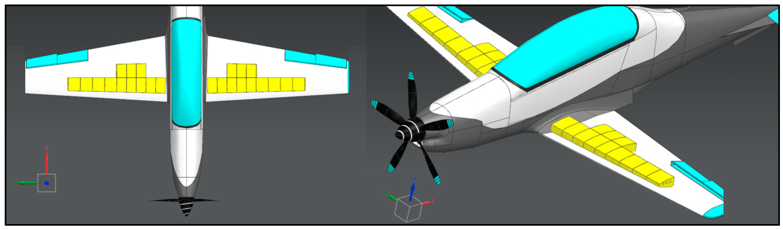
In the stage of tank modeling, storage and fuel distribution in wings are considered. According to the XZ plane, landing gears are assumed to be symmetrically located on both wings. The structural boundaries of wing tanks consist of upper and lower skins of the wing. As a result of the physical restrictions of wing structure, the fuel tank must be allocated with limited shape options. The location of landing gear components is an example of one of these restrictions. Hydraulic and avionics components of the landing gear system cause the fuel tank to have a smaller volume than the entire wing structure. The fuel tanks are allocated on both sides of the aircraft, as shown in
Figure 1.
In the stage of baffle design, fully constrained parametric modeling is conducted to make further changes to the study under control. Fully constrained parametric modeling is mandatory to establish a parameter matrix. That parameter matrix generates a simulation set. There are many holes in the baffles. Gaseous and liquid phases of fluids can flow across the holes. In the current study, cutout divergences, cutout numbers, barrier usage, and diameter of cutouts are taken as geometric design parameters. Additionally, different filling rates are also considered as operational parameters. On the other hand, all fuel tanks also have mouse holes, ventilation holes, and spar holes as a mandatory design feature. However, these mandatory holes have fixed dimensions and do not need to be taken into consideration for parametric studies. Meanwhile, openings for fuel passage, known as mouse holes, are required and should be positioned at the wing’s lower surface corners for each baffle. The term “barrier” refers to a design that has no cutout holes on a baffle but includes all other fixed holes. Fixed holes can provide an advantage in making the 1D model simpler in the following stages. The specific names of features of both baffle and spar design are explained in
Figure 2. This figure is taken for one of the triplet cutout designs as a representation.
For triplet cutout holes, the mid-hole distance
is defined as half of the entire baffle length
. The values
and
represent distances of cutout hole centers from lower points of the front spar and main spar along the
z-axis. For twin cutout hole construction, the baffle gap and distances from two sides of the baffle are equal to each other and also equal to one-third of the
dimension. For a variation of designs of cutout hole allocations, all holes are diverted together when the divergence parameter of
is changed. The single-hole design always centers on cutout location at the beginning of simulations.
Figure 3 shows one sample baffle for all cutout hole amounts. Circular holes and notations of all necessary dimensions are plotted on that baffle sample. This figure is also considered valid for entire baffles on the wing tank.
The
and
notations represent cutout hole diameter and ventilation hole diameter, respectively.
is used for the general notation of cutout hole diameter. The “
ith” baffle in 1D simulations is represented with upper indices of “
i”. From the hub to the tip of the wing, baffle indices are denoted by 1 to 8. The analysis of baffle hole diameters is classified using the grouping method. In this case, the baffle numbering is shown in
Figure 4.
Different designs obtained by changing various parameters require different numerical calculation cases. In this case, numerous analysis outputs are obtained depending on the parameter type and the number of parameters. The amount of CG deviation and retreat time are studied as objective functions concerning hole divergence, barrier usage, cutout quantity, and diameter of circular cutout holes. Divergent cutout holes are created by sliding their centers in the z-direction, as shown in
Figure 4. Only baffles located on the longer side of the tank are considered in this study.
For a mathematical definition of CG, the time-dependent
function is defined by continuous distribution of center of mass formulation. The definition of CG displacement contains only liquid mass because of negligible air density compared to the liquid in this case. The CG of differential mass is integrated over the entire liquid mass along the
y-axis, and the center of mass is achieved for the whole region. The proportion of center of mass to total mass gives CG displacement from the global datum. Consequently, Equation (1) gives a time-dependent center of gravity function along the
y-axis. It is calculated by integrating each element’s CG location and proportion to the entire mass. For each case, the term
is chosen as a maximum deviation in CG and as an output parameter. Another term,
, represents retreat time, which is also selected as another parameter. This assumes that retreat time is the amount of time needed to recover CG divergence 0.20 m away from its initial location after achieving maximum CG. The term
represents peak time, which is assumed to be constant in all cases, equivalent to 10 s, as these values are described in Equation (2). The term
represents time taken to reach 0.20 m from beginning of the analysis, which varies depending on case. Additionally, the mathematical definition of CG deviation is shown in Equation (3). The terms
and
represent fuel’s total and differential mass, respectively.
All the center of gravity deviations are evaluated along the y-axis due to the wing tank shape and bank-to-bank maneuver behavior, and other directions can be neglected for this study. Only a left-wing tank is sufficient to obtain meaningful results due to the symmetry, and all calculations are managed at this tank. Consequently, the CG function is obtained after analyses for the left-wing tank of the aircraft to evaluate CG deviation along the y-axis and retreat time parameters.
3. Methodology
Aircraft have six degrees of freedom when maneuvering because of the nature of flight mechanics and aviation. Therefore, three linear and three angular parameters should be used to define accelerations. All study assumptions are for level flight, except for the roll angle and a specific maneuver known as ‘bank-to-bank maneuver’, which involves a lateral movement of the aircraft’s center of gravity. When no linear accelerations exist, flight is considered in cruise conditions. Fuel travel and sloshing between subsections are triggered during level flight by applying a bank-to-bank maneuver to the entire body. According to Equation (4), initial conditions for Φ (roll), θ (pitch), and Ψ (yaw) angles are taken to be zero for an ideal level flight.
Roll angle gradient is the only tool used for bank-to-bank maneuvering. The input for this maneuver is considered to be a peak roll angle of π/4 radians for 10 s, as represented by the function in
Figure 5. This discrete function is defined to determine the time-dependent equation for roll angle. This function gives angle versus time in radians, as shown in Equation (5).
Pitch and yaw angles remain constant, so their gradients are equal to zero for the entire maneuver, as shown in Equation (6). Compared to the gravitational force acting on fuel mass, centrifugal effects caused by yaw velocity are small enough to be neglected. Initial linear acceleration components and centrifugal forces during maneuver are also assumed to be zero for ideal level flight conditions, as shown in Equation (7). In the equations, the terms
,
, and
represent linear accelerations along x, y, and z axes.
After defining initial values and basic assumptions of mechanics, design and operational parameters are determined. The filling ratios of 30%, 45%, and 60% are considered three different operational parameters for entire simulations, and it is called volume fraction represented by the
term. The parameter matrix is generated by adding design parameters to the volume fraction. These parameters comprise cutout hole diameter, allocation, barrier usage, and cutout hole amount. To make the entire study independent of flow area parameters, twin and single cutout designs are set to calibrated diameters corresponding to the same flow area as the triplet design for each baffle. Because of this calibration, single, twin, and triplet types of cutout holes have different diameter sets of cutout holes. The term
represents cutout hole amount, which is composed of single, twin, and triplet types throughout the study.
Table 1 shows parameter matrices according to these parameter sets. When these parameters are combined, 243 different designs are obtained.
Additional designs with fixed diameter values in all baffle groups are included in this design set. Fixed cutout hole diameters are 50 mm, 60 mm, and 70 mm for these additional designs. The design suggestions include structures without barriers and hole divergence for all three volume fractions. Thus, nine more designs are included, and 1D simulations are carried out for 252 cases. All design cases are provided in “
Appendix A”. These cases are run to reveal the temporal behavior of CG along the
y-axis.
After defining the design matrix, the simulation method and processes are determined. As a 1D modeling tool, the Siemens Amesim solver is chosen to establish a 1D model of the wing fuel tank. Each design feature to be used during 1D modeling represents a mathematical equation. For this reason, all cutout holes, mouse holes, ventilation holes, tank subsections, fuel, and air properties are defined synchronously with each other. Between corresponding subsection control volumes, each hole is represented in the model as an individual orifice equation [
27]. During the calculation stage, these holes are varied to obtain different cases with different designs. The remaining mouse and ventilation holes do not require variation. These non-circular holes are defined with the aid of the CAD Import module of the Amesim program. The advantage of this module is that mouse and ventilation holes are always constant, which reduces computational costs during calculations. In the tank subsections, circular cutout holes, non-circular holes, global fluid parameters, and dynamic parameters are constructed with corresponding constraints in
Figure 6. Bounds between each element represent different submodules of the relevant elements. These bounds are required to build a model at the compilation stage of Amesim. The software manages this step automatically, so choosing the correct bound is enough to construct a 1D model.
When the construction of the 1D model of the entire system is finished, the cases are calculated with relevant input parameters. After achieving the results of 1D simulations, a specific algorithm is required to process output data. The DNN (deep neural network) algorithm is used instead of Multilayer ANN due to the complexity of input parameters. Three hidden layers and six nodes (which can be called neurons) for each hidden layer are programmed as a DNN algorithm for calculations. The primary purpose of examining the results of 1D simulations with the DNN algorithm is to determine the dominance of input parameters on outputs. As a result of this calculation, a numerical result of weights is obtained for each node bound. These weight values indicate the effectivity of bound between relevant nodes. Then, the importance of input parameters over CG deviation behavior is evaluated with specific processes on these weights. Thus, with the help of a suitable DNN algorithm, the importance of input parameters for both CG deviation and retreat time is determined.
To construct an algorithm for DNN structure, specifications of neural networks are defined, such as node numbers, activation functions, input layer, output layer, and hidden layer structures. A suitable DNN algorithm is programmed with Python syntax to solve the outputs of 1D simulations. At the beginning of DNN calculations, inputs and outputs are known for each case. All nodes of hidden layers are also defined as specific functions, and they remain constant for all cases. Weight values must reached specific values after a certain number of iterations with a predefined error rate. All input parameters, weight tensors, hidden layers, function names, and outputs are named, as seen in
Figure 7. Dashed lines and spherical elements represent weights and nodes, respectively.
Nodes of the input layer are composed of operational and design parameters, as mentioned before. On the other hand, the output layer contains maximum CG deviation and retreat time. As stated in “
Appendix B”, the weight tensors of the 1st, 2nd, 3rd, and 4th groups are represented with
,
,
, and
, respectively. Each tensor has weight elements represented by
, and indices of
,
, and
k represent the number of target nodes, departure nodes, and weight groups. Three different activation functions are chosen for each hidden layer individually. The sigmoid function, hyperbolic tangential function, and ReLU (Rectified Linear Unit) function are chosen for the first, second, and third hidden layer nodes, respectively. Activation functions are defined in Equations (8)–(10).
Calculation inputs and results are implemented into the DNN algorithm. Then, learning iterations become ready to start with learning rate, epoch number, and batch size, which are set at 0.0012, 10,000, and 25, respectively. These values are determined by targeting the difference between predicted and learned values as 1% at maximum.
After weight calculations, weight values must be interpreted. By interpreting weight values, the direct dominances between input parameters and outputs are obtained numerically. Garson’s interpretation algorithm can be used for this modification process [
28]. This algorithm is conducted with all weight values, and the importance of input values is evaluated with Equation (11).
In Equation (11), the terms “
”, “
”, and “
” represent the number of input neurons, number of hidden neurons, and dominance of relevant input layers, respectively. The weight terms are denoted by
and written as a tensor form in “
Appendix B”. This operation is processed for each input parameter, and as a result of this calculation, five dominance values are obtained individually.
There must be a single-layer ANN structure instead of the complex structure of DNN. In this case, the hidden layer structures should be modified into a single hidden layered structure. Kamimura’s study mentions that a specific compression algorithm converts the DNN structure into a temporary single-layer ANN [
29]. Thanks to the relevant compression algorithm, this temporary ANN structure can be considered equivalent to the main DNN structure in terms of the impact of inputs. For the compression process, the weight matrix of the layers of
and
is multiplied and then summed for each node. By carrying out this step, the weight matrix between the first compressed hidden layer and an output layer of
is generated. After the first compressing step, the recently obtained weight matrix of
is the new weight matrix between the output layer and hidden layer before the output layer. The same step is applied again between
and
to advance the compression process one step more. After the second compression step, the weight matrix
is obtained as a weight structure between the output layer and the layer before it. The compression of hidden layer operations can be expressed mathematically for all steps, respectively, as shown in Equations (12) and (13).
After two steps of compression, the process yields a compressed single-layer ANN with weight matrices of and . This compressed ANN structure is chosen to interpret weights using Garson’s algorithm. The interpretation of weights is obtained using Equation (11), which gives the importance of each input parameter individually. In light of the importance of the results, the dominance of input parameters on results is evaluated.
A detailed numerical calculation is conducted after calculating 1D simulations and weight importance values. In light of results obtained from 1D simulations and ANN calculations, certain cases are chosen to be examined in detail. Cases selected for these examinations are managed with 3D calculations. The CFD methods are used to process these calculations. Conducting CFD simulations for these cases aims to obtain detailed outcomes and compare them with the 1D results and parameter dominances of the same cases. At the stage of CFD calculations, the Siemens StarCCM+ flow solver program is used to construct and run calculation cases. Similar to the 1D simulations, solution intervals of 100 s are assumed as a transient domain of calculation. Calculation processes are managed with an HPC (High-Performance Computer) server, and this hardware has provided the ability to handle high computational costs for many a grid structure.
Model construction of the entire calculation is carried out with certain assumptions. The whole study is conducted under isothermal conditions, and all regions are assumed to have cruise conditions of 250 K temperature. Heat dissipation and bubble generation effects are small enough to be neglected at the phase interaction region. The fluid’s liquid phase is JP8 (Jet Propellant 8), and the gaseous phase of fluid is defined as air. The software material library already includes properties of ideal gas air, and JP8 is manually defined with specific properties such as density and dynamic viscosity, 840 kg/m
3 and 0.003 Pa.s, respectively. The remaining model construction attributes are briefly charted in
Table 2.
Additionally, phases have an interaction of free surfaces between each other, which must be defined. Specific definitions are imported into the program to model phase interaction between fluids. The surface tension force definition is chosen to determine the interaction behavior between both phases, and it is defined as equal to 0.025 N/m. On the other hand, the AMR function is programmed to perform periodically at every 20 ms of physical time. When this function is triggered, the free surface mesh structure is updated in parallel with the change of free surface. In addition, the adaptive time step is programmed according to certain limits. These limits are maximum CFL (Courant–Friedrichs–Lewy) conditions for interior flow and free surface. According to the maximum CFL condition limits, the Courant number of interior and free surface flows is forced to remain less than Co = 0.75. Thus, adaptive time step programming prevents the transient solution from behaving as unstable.
After case construction, a reference model is determined to check if it is progressing without any calculation divergence. Additionally, a reference case is used to finalize the mesh structure of the wing tank interior volume with the aid of a mesh independence study. “Case 3”, stated in “
Appendix A”, is selected as a reference case to control calculation case functionality and conduct mesh independence. Specifications of the chosen case are briefly written down in
Table 3.
When the appropriate case is created and the mesh independence study is completed, other analyses can be organized through this case structure. At this step, a base CFD case file is obtained and preserved to generate other CFD calculation cases with only the required parameter variation. After the results of 1D simulations and DNN calculations are obtained, additional CFD solutions are planned to be conducted. Thus, the precision of 1D simulations and the accuracy of DNN results are controlled with additional CFD results.
4. Results
The results were obtained in planned order, the same as the progressing queue of the methodology. The queue is first to complete 1D simulations and record the results, then to analyze these results with the DNN algorithm, and finally to verify chosen cases in CFD calculations.
4.1. The 1D Simulation Results
The 1D analyses were carried out sequentially from case 1 to case 252. Retreat time and maximum CG deviation parameters were extracted from the transient CG function obtained from 1D simulations. The results were obtained relative to the initial CG displacement of each case. Thus, the initial value of CG deviation in all results was 0 m. Transient CG functions
are shown in
Figure 8. In this graph, one of the horizontal axes represents the physical time from the initial value to the end of simulations, which are t = 0 s and t = 100 s, respectively. The other horizontal axis shows case numbers from 1 to 252. The vertical axes and chart legend represent the amount of CG deviation depending on time.
The graph is useful to observe changes in CG behavior depending on parameter variations. However, the definition of retreat time and maximum CG deviation require numerical values from the results of analyses. All case numbers, parameter attributes of these cases, and case results are stated in “
Appendix A” individually. An alternative representation was used to make values on the chart easier to examine. The output data were nondimensionalized to use this alternative representation. Both parameters were created in non-dimensional form in order to observe results in one 2D graph. Maximum CG deviation and retreat time were nondimensionalized, as in Equations (14) and (15), respectively. The terms of
and
represent nondimensional values of maximum CG deviation and retreat time, respectively. These nondimensional definitions were achieved by normalizing them with the values
and
, which represent maximum
and maximum
for all cases, respectively.
The results close to 1 mean a higher maximum CG deviation and retreat duration, and results close to 0 imply the opposite. The dimensionless CG deviation and retreat time results were obtained for 252 cases, as shown in
Figure 9, and values close to zero for each output are determined as targets for both output parameters.
As can be seen from the results of 1D simulations, CG deviation and retreat time outputs are acting as conflicting parameters. Input parameters that increase the CG deviation value show the effect of shortening retreat duration. Similarly, parameters that act to reduce CG deviation value also extend retreat duration. Volume fraction has a significant impact on the behavior of CG deviation, as it is directly related to the weight of fuel. It is observed that a lower volume fraction of fuel causes greater maximum CG deviation. Barrier usage is also another cause of variations in CG behavior. Because barriers have only ventilation and mouse holes instead of additional cutout holes, barriers cause greater resistance against flow between subsections. Increasing cutout hole diameters causes the CG deviation to increase as well, because this change reduces the pressure drop of orifices in the transition between subsections. When the divergence of the cutout hole is negative, the CG deviation value increases and the retreat time value decreases. The reason for the decreasing position of the cutout hole along the z-axis is that it changes the hydrostatic pressure difference between two sides of the cutout hole.
4.2. DNN Results
Input parameter effects were evaluated briefly from 1D simulation results. However, a detailed evaluation was performed in order to examine the parameter dominance of inputs over results. Because the dominances are required to determine parameters, they should be changed primarily in order to obtain better results from the design. The outputs obtained from 1D simulations were analyzed with the DNN algorithm. The aim is to obtain weight values of the whole neuron bounds of the DNN structure related to the 1D results.
Relative error monitoring was performed to verify the precision of results after iterations. The difference between results from 1D simulations and the results learned by the DNN algorithm was calculated. By comparing these differences, relative error values were calculated. Individual relative error values were defined as and for CG deviation and retreat time, respectively. When the relative error rate between these results reached 1%, iterations of the DNN algorithm were terminated. Relative errors were calculated as 0.56% for and 1.00% for values.
In all 1D simulations, results for each parameter and results taught to the DNN algorithm are compared as shown in
Figure 10. Trendlines of cumulative results are represented with
and
functions for deviation results and retreat time results, respectively. The reason why results obtained for retreat time are more scattered than CG deviation is the criterion determined for this parameter. This criterion is the time taken to reach 15 cm CG distance from the initial location for all cases. This was chosen as a constant rather than a ratio of maximum CG deviation to be an independent parameter.
The results have shown that the estimated outputs of 1D simulations were correctly predicted by the DNN algorithm. The effect of all parameter combinations on results was obtained with an acceptable error rate. The number of analyses used as input was determined as 252. Increasing the number of analyses would enable the algorithm used to reach desired results with a lower number of iterations or a simpler ANN algorithm. As noted in “
Appendix B”, the weight values of each neuron bound were obtained from calculations.
Before the weight interpretation step, a DNN compression process was carried out. As a result of DNN compression, a temporary ANN structure has been achieved. Weight interpretation processes were conducted with the aid of MATLAB in order to handle hundreds of sequential iterations. The dominance of each input on outputs was obtained and the results of the importance of inputs are shown in
Figure 11.
As a result of the weight interpretation of the neural network, it has been clearly shown that the barrier usage of the tank has the strongest importance for both CG deviation and retreat time. Additionally, volume fraction, cutout hole diameter, and cutout hole divergence parameters were shown as second, third, and fourth dominant inputs on both outputs, respectively. Lastly, the hole number was shown to be the parameter with the least impact. On the other hand, the parameters had a similar effect on both outputs. This situation can be explained by the fact that the amount of CG deviation has a significant effect on the behavior of retreat duration. As a consequence, barrier usage was a design parameter that was observed as the most dominant parameter in both CG deviation and retreat time. However, the volume fraction was an operational parameter that has been calculated as the second most dominant parameter. Unlike the operational parameter, the design parameters are suitable for optimization in order to obtain better solutions during the design of the tank. Yet, the volume fraction cannot be constant in certain values as a result of engine fuel consumption during flight. Operational parameter results are useful for estimating sloshing effects on relevant volume fractions.
4.3. CFD Results
After 1D simulations and detailed parameter analyses were finished, CFD analyses started progressing. All cases were calculated with HPC, which has 640 core processors and 448 gigabytes of available memory. Whether there was any error in the analyses was checked simultaneously while the analysis was ongoing. The CG deviation function, which is controlled during the calculation, was manually implemented into the software according to Equation (1). CG deviation and retreat time values were extracted from the results of these functions.
By performing a mesh independence study, it was guaranteed that the analyses would not give diverged results due to the case grid structure. The grid structure obtained from this study was accepted as a mesh for all CFD analyses. The CG behavior was chosen as a control parameter to be used to check the reliability of different grid structures. The mesh independence study was conducted with six runs of these different grid structures. The approximate element numbers of related grid structures were 300 k, 600 k, 1.7 M, 3.0 M, 5.0 M, and 39.0 M, respectively. Additionally, the AMR method was used for cases that have 3.0 M, 5.0 M, and 39.0 M cells. The AMR was used for these cases in order to capture free surface turbulence while avoiding excessive increases in the number of elements of the entire volume.
For the reference case, a polyhedral grid structure generated with 5.0 M cells is shown in
Figure 12 as an example. In the figure, the section view of the meshed volume is named section A-A. In the section, the inflation of surface meshing and polyhedral structure are shown. Additionally, the grid structure initially refined by AMR around the free surface is seen in section A-A. Thus, the grid structure of the figure represents the volume mesh at t = 0 s. The volume fraction of the reference case is 60%, and the relevant free surface level is also shown.
Variations in grid structure resulted in numerical results. Only the interval between the 0th and 40th second of the temporal region was chosen because major differences were shown in this interval. The calculations showed negligible differences from grid structures larger than 5.0 M element count. The numerical results of mesh independence calculations for each grid structure are stated in
Figure 13.
As a consequence of this study, a grid structure constructed with 5.0 M cells was chosen as the main grid structure. Thus, ongoing CFD calculations using this grid structure were considered independent of the mesh.
After mesh independence calculations, mesh-independent CFD calculations were run. In order to evaluate the output difference between 1D and CFD results, a reference case has been chosen as an initial case run. It was deemed appropriate to examine the free surface structure to observe the differences between CFD and 1D results. The post-process outputs of reference cases with different solution times are shown in
Figure 14. In this figure, the left column contains CFD results, and the right column contains 1D simulation results.
The most obvious difference between these two types of solution method is shown in the free surface of the fuel volume. Free surface behavior is turbulent in CFD results; on the other hand, 1D simulation results show smooth planes with a certain altitude angle for each subsection.
In addition to the visual outputs, CG deviation functions of both 1D simulation and CFD calculations were obtained for numerical evaluation of the reference case. The reference case results of both 1D and CFD calculations are shown in
Figure 15.
As shown in the results of the reference case, CFD and 1D simulations of the reference case have slight differences. The evident differences between numerical results are observed around the peak point of the CG deviation function. This is an understandable result, because the differences between CFD and 1D simulation become easier to detect where turbulence increases. The interval where turbulence increases is the interval where the maneuver is applied. After the maneuver is finished and the flight condition returns to cruise conditions, the differences between CFD and 1D simulation outputs are dissipated.
In addition, according to the results in
Figure 9, three cases with the highest and three cases with the lowest nondimensional values were selected and analyzed. With these additional calculations, the aim was to evaluate the results of the best and worst cases and the effects of their input parameters on calculations. Determined cases and their parametric specifications are shown in
Table 4.
The analyses for these cases were made using exactly the same method as reference case calculation. The numerical results of the CG deviation function for these six cases are plotted in
Figure 16.
When the results were examined, it was seen that there were slight differences between 1D simulations and CFD analyses, similar to the results of the reference case. These variations are also mainly due to the difference in solution methods. Consequently, there are some differences between the free surface modeling of 1D and CFD solutions. In 1D simulations, each subsection of tank volume is filled with fluid theoretically using the control volume method. Although the visual outputs are generated with the Amesim v2019-2 software’s CAD import module, solutions are conducted only by solving the sequence of mathematical equations. On the other hand, the method of CFD solutions is processed by the finite volume method, which is generated by dividing the entire geometry into differential elements. Each cell of the grid structure represents a different control volume. As a result of these significant differences, these two solution methods produce different results of free surface behavior. The effect of turbulence considered on the free surface is not simulated in 1D analyses as a result of its solution method. This situation affects the orifice modeling between subsections with different hydrostatic pressure differences. This circumstance can explain different results obtained with maximum deviation amounts. On the other hand, it is observed that precise CFD results are achieved with the 1D solution method without any excessive error rates.
Other additional CFD analyses were planned to control the importance results obtained in the DNN calculations. These analyses were divided into groups to observe the effect of each input parameter individually. Case groups were created so that all parameters were kept constant except the parameter whose effect was under evaluation. In order to control the cutout hole amount parameters, the 10th, 91st, and 172nd cases were selected for calculation. Likewise, the 16th, 43rd, and 172nd cases for barrier usage, 3rd, 6th, and 9th cases for volume fraction, 4th, 5th, 6th, 19th, 22nd, and 25th cases for cutout hole diameter, and finally, 97th, 98th, and 99th, cases for cutout divergence control were selected. The results of CFD calculations of these cases were obtained.
According to the results obtained for barrier usage in
Figure 17, it is seen that the design using a barrier is quite effective for CG deviation behavior compared to the design without a barrier. However, if the barrier is used on different baffle elements, there are not any significant differences between results. Thus, it seems that the number of barriers is much more effective than the baffle number at which the barrier is applied.
The volume fraction is included in the calculations as an operational parameter, unlike other design parameters, as mentioned before. After the examination of results, the effect of the volume fraction parameter is clearly noticeable in
Figure 18. When the differences in results are examined, it is observed that the maximum CG amount increases as volume fraction value decreases. This situation can basically be explained as a result of the effect of the same maneuver on different masses of fuel.
A comparison of different cutout hole diameter values is conducted for this set of analyses. This comparison includes designs where the same diameter values are used throughout the entire wing, as well as cases where various diameter values are used in different baffle groups. The sensitivity of output parameters to the change in cutout hole diameters can be observed in
Figure 19. The effect of diameter values is seen as the most effective parameter after volume fraction and barrier usage parameters.
The effect of the divergence of the cutout hole parameter on outputs is not quite dominant, as shown in
Figure 20. However, it is still detected that maximum CG deviation and retreat duration outputs are affected by these parameters. Although it does not have as dominant an effect as other parameters, the cutout divergence effect cannot be neglected in light of these results.
As can be seen from the results in
Figure 21, the use of different numbers of cutout holes barely affects the results. The effects of the number of cutout holes on baffle performance can be neglected as long as the amount of flow area does not change. As a result, hole numbers are an important parameter for structural design restrictions instead of CG deviation behavior.
5. Conclusions
The study utilized the geometry of a training aircraft tank instead of a simplified tank geometry, considering the practical constraints in the industry. This article proposes the examination method of 1D and CFD simulations with the help of DNN, where different results are obtained with high amounts of input combinations. While determining this method, 1D and CFD simulations consist of fuel sloshing in an aircraft wing fuel tank. Numerous analyses are composed of the combination of different input parameters, including cutout hole amount, barrier usage, volume fraction of fuel, cutout hole diameter, and cutout hole divergence at the interior volume of tank structure. Analyses are conducted under the effect of certain maneuvers, and then two output parameters of maximum CG deviation and retreat time are calculated. The results of 1D simulations of 252 different parameter combinations compose the input data for detailed examination with the DNN structure. With the use of an artificial intelligence-based algorithm, the importance of input parameters over outputs is obtained numerically. Additionally, the double-checking of results of importance values is conducted with the aid of 3D calculation results of the CFD method.
The 1D simulations are compared with CFD calculations of relevant cases, and there is acceptable agreement between them. Thus, 1D simulations can be assumed to be reliable unless extreme maneuver conditions are implemented into analyses, such as barrel roll or wingover maneuvers of fighter jets, which have greater acceleration than 0.5 times the gravitational acceleration “g” along the y-axis. The unsteady behavior of CG deviation and retreat duration can be predicted from 1D simulations at a much lower computational cost. According to the results, the analysis amount can be increased in order to simulate the effects of additional parameters such as individual baffle design and variations of mouse holes. With the aid of the DNN algorithm, a higher amount of analysis can be processed, and even design proposals can be extracted from the enhanced DNN algorithm.
The provided investigations pertaining to the tank illustrate fuel slosh in the wing tank and demonstrate the effects of baffles on fluid dynamics in detail. According to the results of the study, it was observed that the input parameters affect the CG deviation and the retreat time similarly when designing a baffle for a wing tank; therefore, it is recommended that the barrier design be taken into consideration as a priority. Volume fraction has the second greatest dominance over both outputs as an operational parameter of the fuel tank. However, the volume fraction should not be viewed as a design parameter, but rather as an operational parameter. Cutout hole diameter, cutout divergence, and number of cutout holes as input parameters are listed in descending order of importance. In conclusion, the study presents a methodology to comprehensively examine a large number of simulations to analyze the effect of fuel sloshing in research on baffle design within a tank and will serve as baffle design proposals for simulations focusing on entire flight stability in future studies.


