
High-Resolution Wavenumber Bandpass Filtering of Guided Ultrasonic Wavefield for the Visualization of Subtle Structural Flaws

 ,
,  ,
,  and
and
Abstract
:1. Introduction
2. Materials and Methods
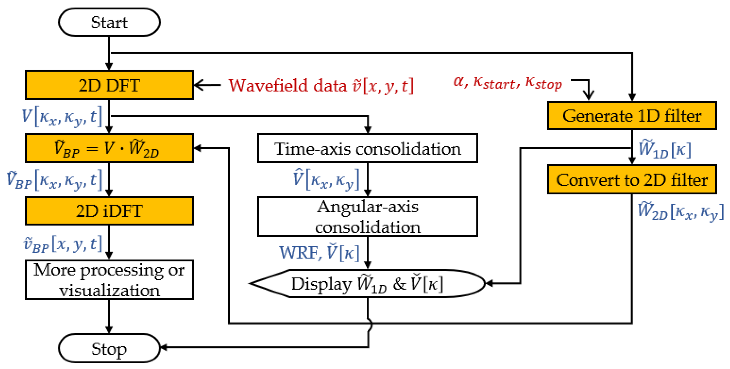
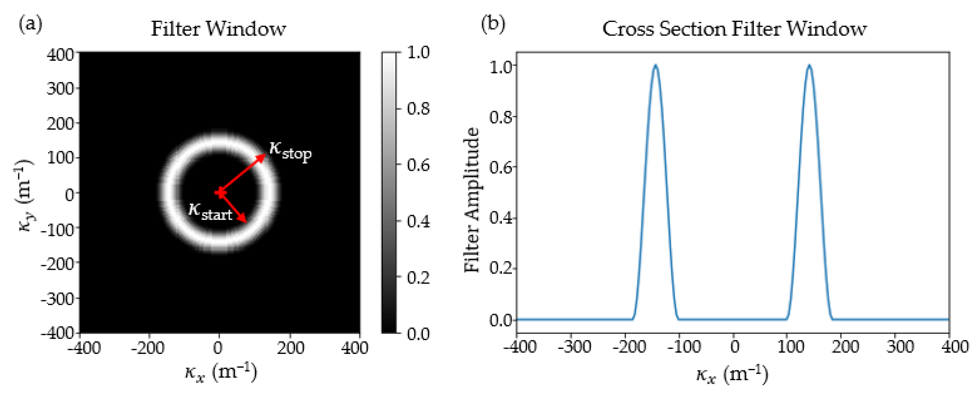
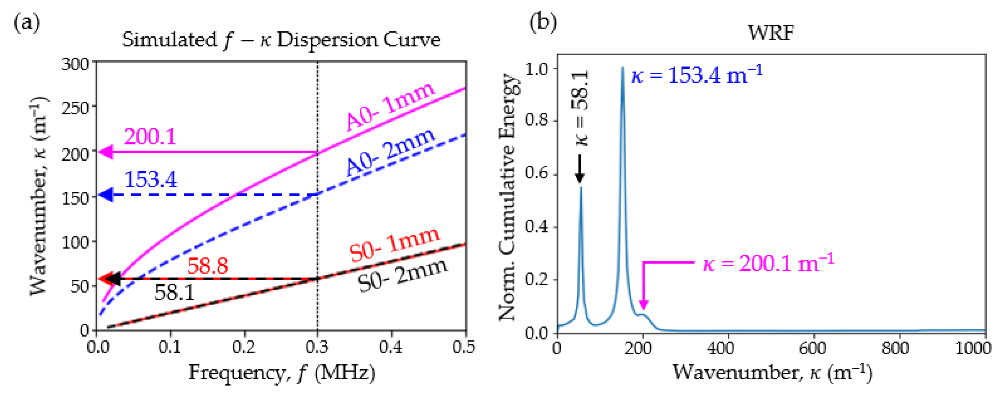
2.1. The Proposed Wavenumber Bandpass Filter
2.2. Specimens and Flaws
2.3. Data Acquisition
3. Results
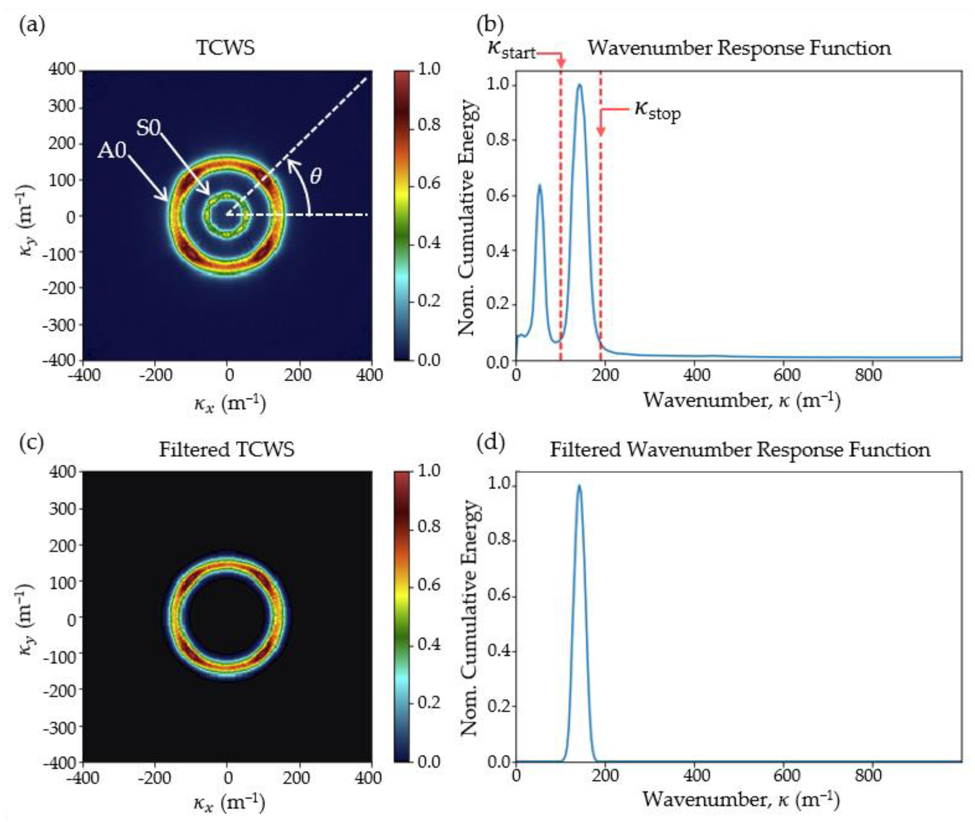
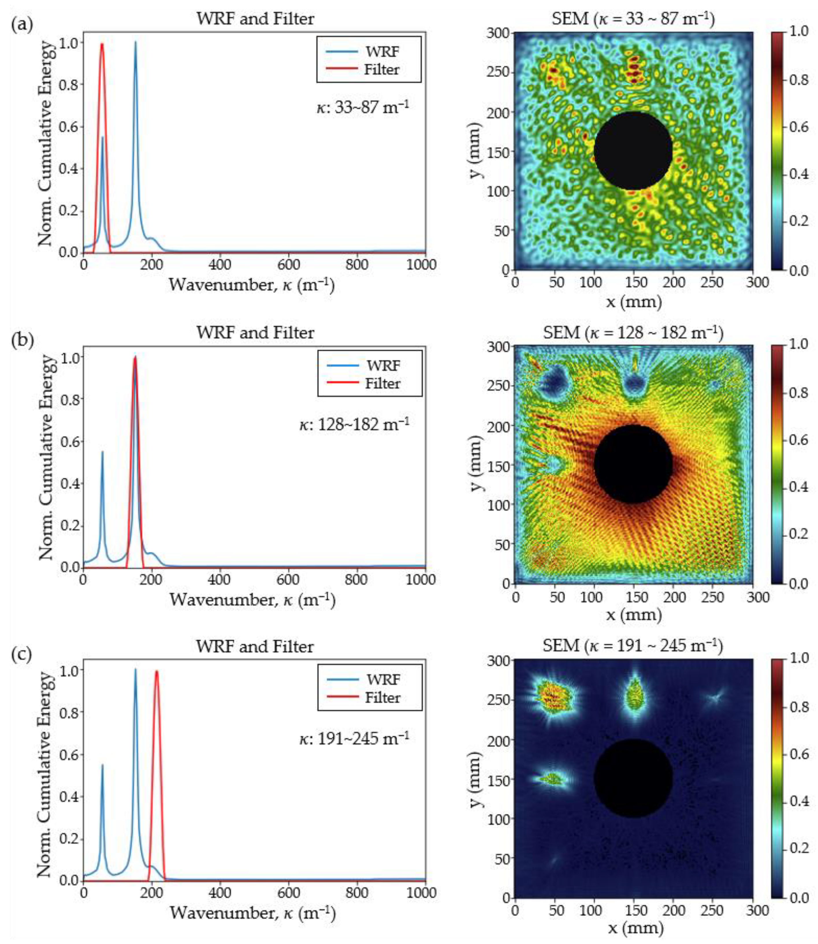
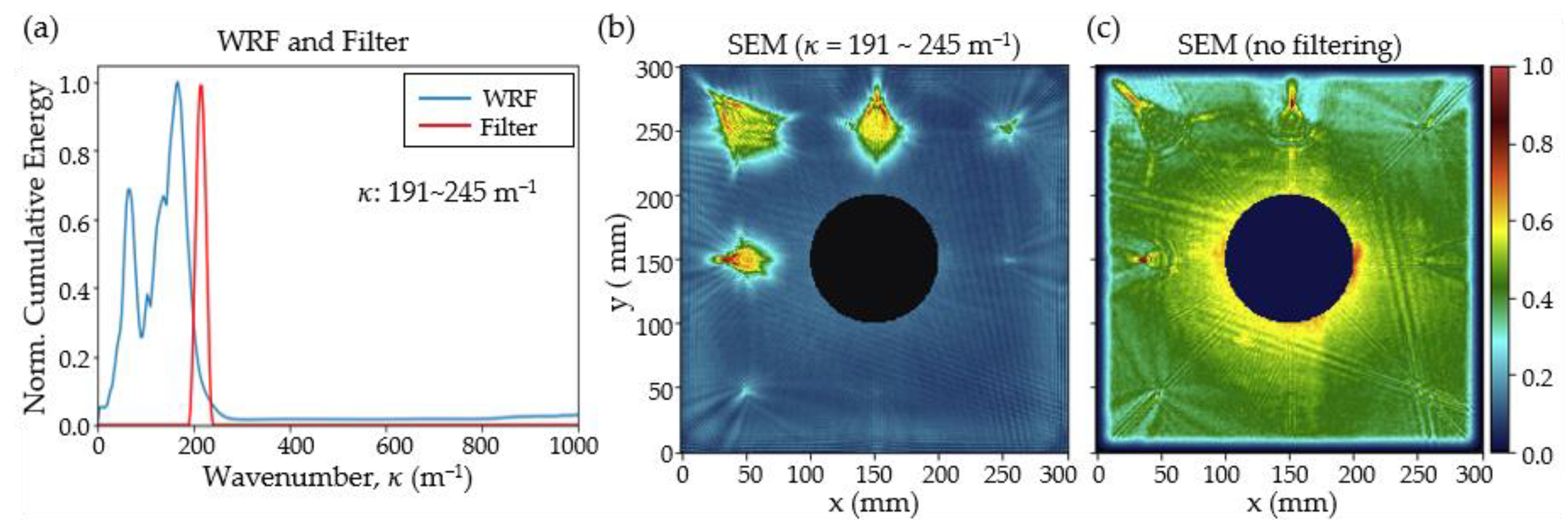
3.1. Validation of Filter Functionality
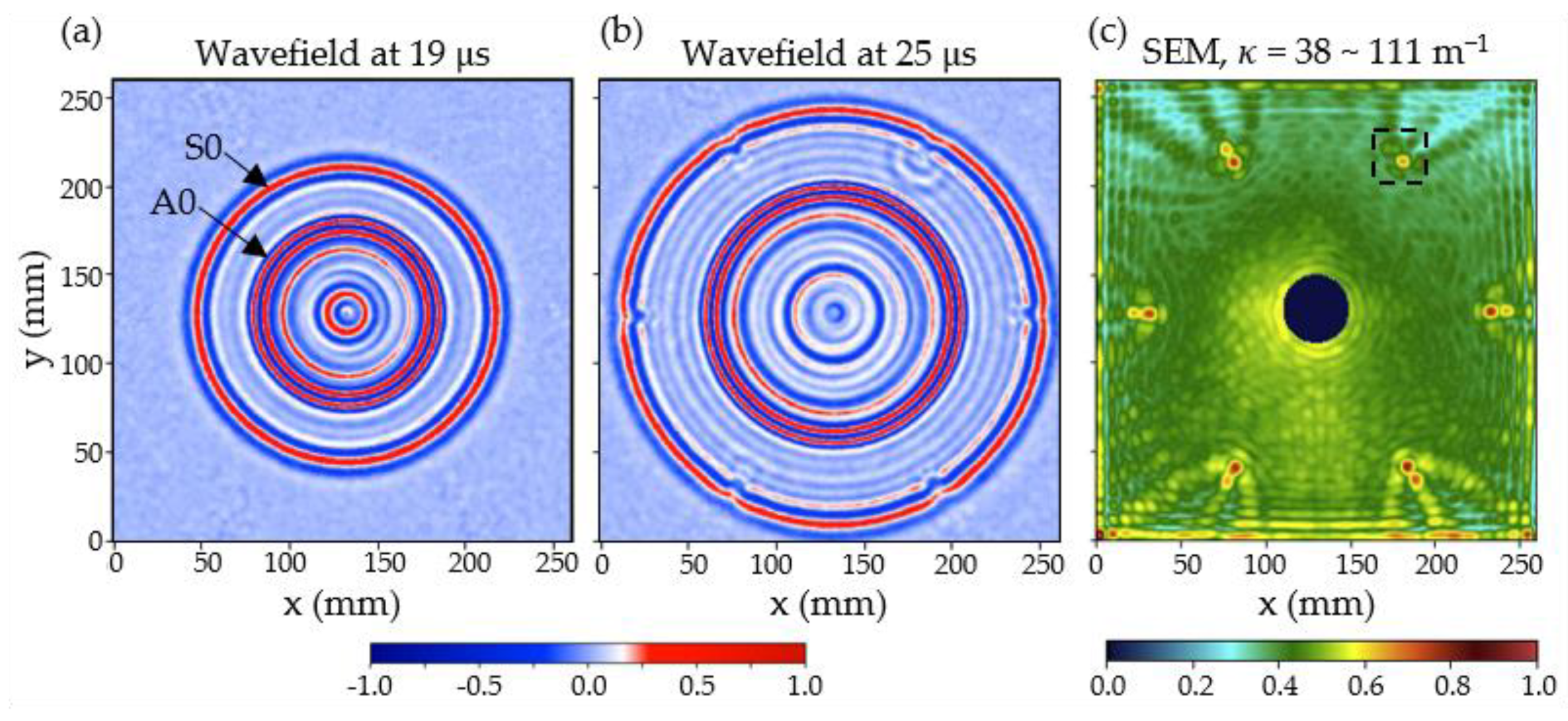
3.2. Consolidation of Information across Frequencies
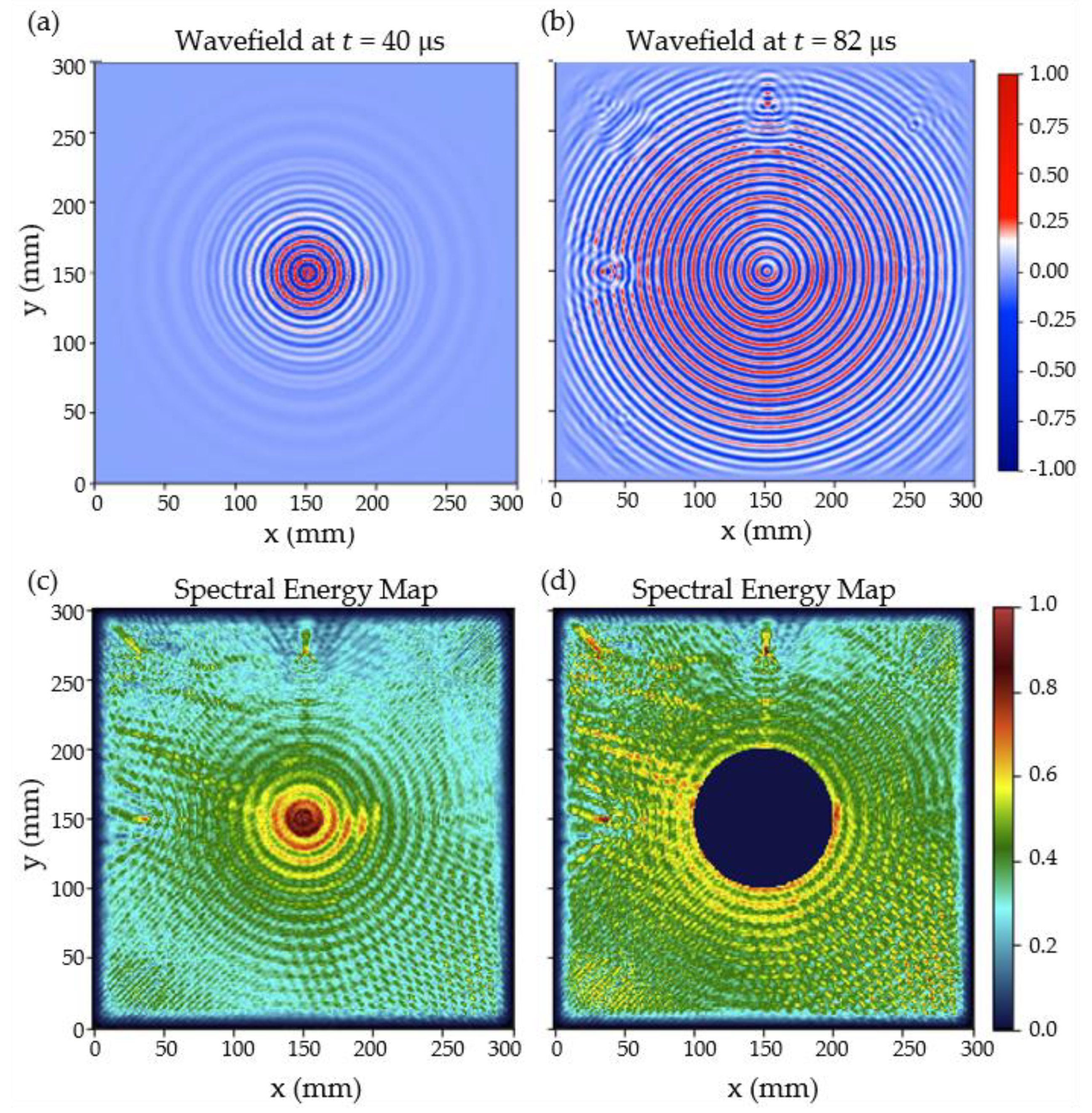
3.3. Evaluation of Subtle Flaws
4. Discussion
4.1. Comparison with Mode Filter
4.2. Principle of Flaw Visibility
4.3. Window Shape and Size
4.4. Detectability of Flaws
4.5. Optimization of Wavenumber Bandpass Range
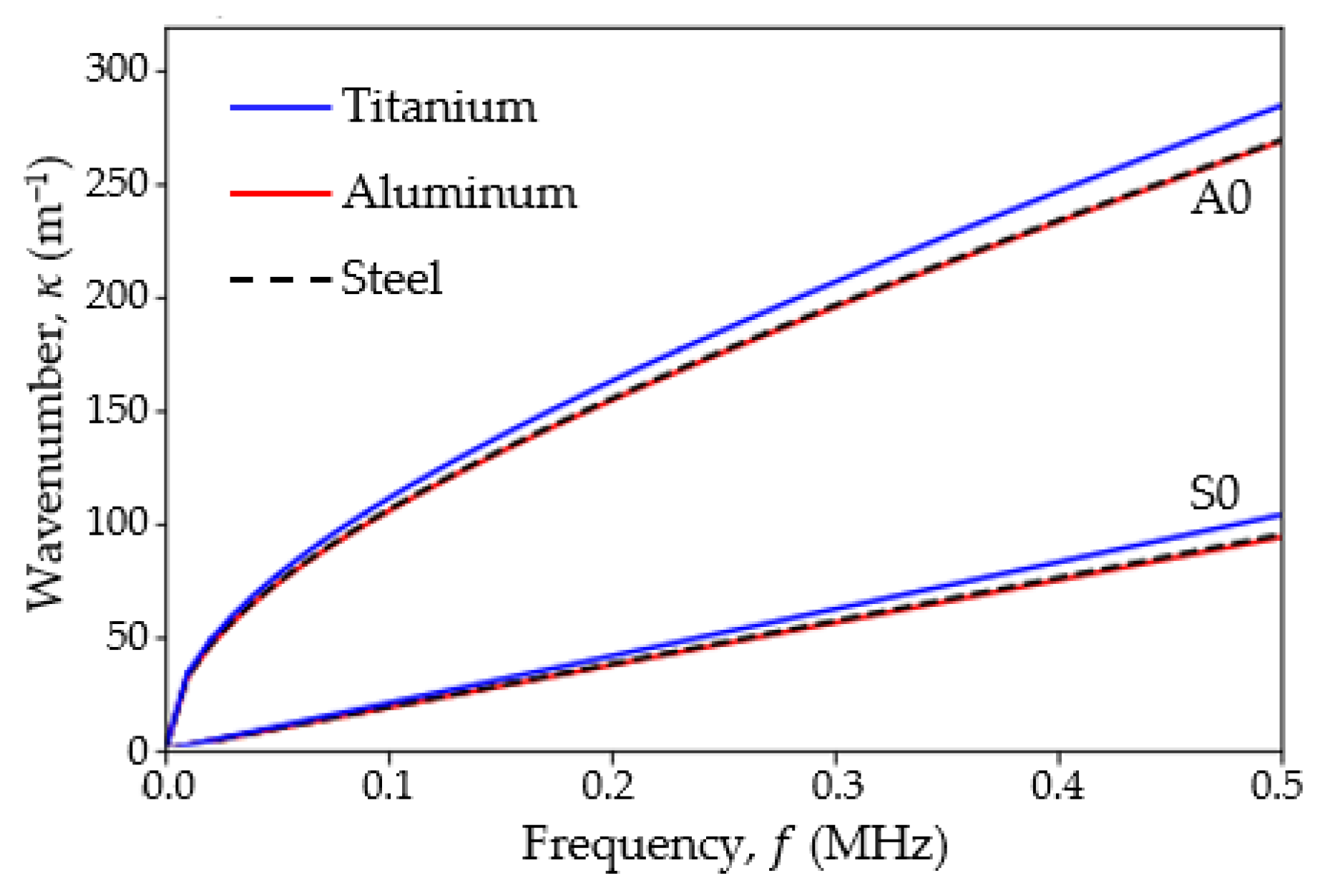
4.6. Suitability for Different Materials
4.7. Masking of Wavefield Source
4.8. Source Positioning
5. Conclusions
Author Contributions
Funding
Data Availability Statement
Acknowledgments
Conflicts of Interest
References
- Chia, C.C.; Lee, S.Y.; Harmin, M.Y.; Choi, Y.; Lee, J.-R. Guided Ultrasonic Waves Propagation Imaging: A Review. Meas. Sci. Technol. 2023, 34, 052001. [Google Scholar] [CrossRef]
- Zheng, S.; Luo, Y.; Xu, C.; Xu, G. A Review of Laser Ultrasonic Lamb Wave Damage Detection Methods for Thin-Walled Structures. Sensors 2023, 23, 3183. [Google Scholar] [CrossRef] [PubMed]
- Chia, C.C.; Jang, S.-G.; Lee, J.-R.; Yoon, D.-J. Structural Damage Identification Based on Laser Ultrasonic Propagation Imaging Technology. In Optical Measurement Systems for Industrial Inspection VI; International Society for Optics and Photonics: Bellingham, WA, USA, 2009; Volume 7389, p. 73891S. [Google Scholar]
- Viktorov, I.A. Rayleigh and Lamb Waves: Physical Theory and Applications; Ultrasonic Technology; Plenum Press: New York, NY, USA, 1967; ISBN 978-0-306-30286-2. [Google Scholar]
- Rose, J.L. Ultrasonic Guided Waves in Solid Media; Cambridge University Press: Cambridge, UK, 2014; ISBN 978-1-107-04895-9. [Google Scholar]
- Dawood, S.D.S.; Harithuddin, A.S.M.; Harmin, M.Y. Modal Analysis of Conceptual Microsatellite Design Employing Perforated Structural Components for Mass Reduction. Aerospace 2022, 9, 23. [Google Scholar] [CrossRef]
- Dong, Z.; Wang, Z.; Tian, J.; Kang, R.; Bao, Y. Investigation on Tearing Damage of CFRP Circular Cell Honeycomb in End-Face Grinding. Compos. Struct. 2023, 325, 117616. [Google Scholar] [CrossRef]
- Lyu, Y.; Niu, Y.; He, T.; Shu, L.; Zhuravkov, M.; Zhou, S. An Efficient Method for the Inverse Design of Thin-Wall Stiffened Structure Based on the Machine Learning Technique. Aerospace 2023, 10, 761. [Google Scholar] [CrossRef]
- Dawood, S.D.S.; Harmin, M.Y.; Harithuddin, A.S.M.; Chia, C.C.; Rafie, A.S.M. Computational Study of Mass Reduction of a Conceptual Microsatellite Structural Subassembly Utilizing Metal Perforations. J. Aeronaut. Astronaut. Aviat. 2021, 53, 57–66. [Google Scholar] [CrossRef]
- Chan, Y.N.; Harmin, M.Y.; Othman, M.S. Parametric Study of Varying Ribs Orientation and Sweep Angle of Un-Tapered Wing Box Model. Int. J. Eng. Technol. 2018, 7, 155–159. [Google Scholar] [CrossRef]
- Rucka, M.; Wojtczak, E.; Lachowicz, J. Damage Imaging in Lamb Wave-Based Inspection of Adhesive Joints. Appl. Sci. 2018, 8, 522. [Google Scholar] [CrossRef]
- Wang, J.; Shen, Y. An Enhanced Lamb Wave Virtual Time Reversal Technique for Damage Detection with Transducer Transfer Function Compensation. Smart Mater. Struct. 2019, 28, 085017. [Google Scholar] [CrossRef]
- Wang, X.; Cai, J.; Zhou, Z. A Lamb Wave Signal Reconstruction Method for High-Resolution Damage Imaging. Chin. J. Aeronaut. 2019, 32, 1087–1099. [Google Scholar] [CrossRef]
- Kang, T.; Yoon, M.; Han, S.; Kim, K.-M.; Koo, B. Selection of Optimal Exciting Frequency and Lamb Wave Mode for Detecting Wall-Thinning in Plates Using Scanning Laser Doppler Vibrometer. Measurement 2022, 200, 111676. [Google Scholar] [CrossRef]
- Chen, H.; Ling, F.; Zhu, W.; Sun, D.; Liu, X.; Li, Y.; Li, D.; Xu, K.; Liu, Z.; Ta, D. Waveform Inversion for Wavenumber Extraction and Waveguide Characterization Using Ultrasonic Lamb Waves. Measurement 2023, 207, 112360. [Google Scholar] [CrossRef]
- Kang, T.; Han, S.-J.; Han, S.; Kim, K.-M.; Kim, D.-J. Detection of Shallow Wall-Thinning of Pipes Using a Flexible Interdigital Transducer-Based Scanning Laser Doppler Vibrometer. Struct. Health Monit. 2022, 21, 2688–2699. [Google Scholar] [CrossRef]
- Xia, R.; Wang, W.; Shao, S.; Wu, Z.; Chen, J.; Zhang, X.; Li, Z. Mode Purification for Multimode Lamb Waves by Shunted Piezoelectric Unimorph Array. Appl. Phys. Lett. 2023, 122, 201703. [Google Scholar] [CrossRef]
- Huke, P.; Schröder, M.; Hellmers, S.; Kalms, M.; Bergmann, R.B. Efficient Laser Generation of Lamb Waves. Opt. Lett. 2014, 39, 5795–5797. [Google Scholar] [CrossRef]
- Rothe, S.; Daferner, P.; Heide, S.; Krause, D.; Schmieder, F.; Koukourakis, N.; Czarske, J.W. Benchmarking Analysis of Computer Generated Holograms for Complex Wavefront Shaping Using Pixelated Phase Modulators. Opt. Express 2021, 29, 37602–37616. [Google Scholar] [CrossRef] [PubMed]
- Kim, T.; Chang, W.-Y.; Kim, H.; Jiang, X. Narrow Band Photoacoustic Lamb Wave Generation for Nondestructive Testing Using Candle Soot Nanoparticle Patches. Appl. Phys. Lett. 2019, 115, 102902. [Google Scholar] [CrossRef]
- Liu, Z.; Shan, S.-B.; Dong, H.-W.; Cheng, L. Topologically Customized and Surface-Mounted Meta-Devices for Lamb Wave Manipulation. Smart Mater. Struct. 2022, 31, 065001. [Google Scholar] [CrossRef]
- Jeon, J.Y.; Kim, D.; Park, G.; Flynn, E.; Kang, T.; Han, S. 2D-Wavelet Wavenumber Filtering for Structural Damage Detection Using Full Steady-State Wavefield Laser Scanning. NDT E Int. 2020, 116, 102343. [Google Scholar] [CrossRef]
- Michaels, T.E.; Michaels, J.E.; Ruzzene, M. Frequency–Wavenumber Domain Analysis of Guided Wavefields. Ultrasonics 2011, 51, 452–466. [Google Scholar] [CrossRef]
- Flynn, E.B.; Chong, S.Y.; Jarmer, G.J.; Lee, J.-R. Structural Imaging through Local Wavenumber Estimation of Guided Waves. NDT E Int. 2013, 59, 1–10. [Google Scholar] [CrossRef]
- Chia, C.C.; Gan, C.S.; Gomes, C.; Mazlan, N.; Gomes, A. Lightning Damages in Glass Fiber-Epoxy Composite Material Used for Aerospace Applications. In Proceedings of the 2018 34th International Conference on Lightning Protection (ICLP), Rzeszow, Poland, 2–7 September 2018; pp. 1–4. [Google Scholar]
- Moon, S.; Kang, T.; Han, S.-W.; Jeon, J.-Y.; Park, G. Optimization of Excitation Frequency and Guided Wave Mode in Acoustic Wavenumber Spectroscopy for Shallow Wall-Thinning Defect Detection. J. Mech. Sci. Technol. 2018, 32, 5213–5221. [Google Scholar] [CrossRef]
- Gan, C.S.; Chia, C.C.; Tan, L.Y.; Mazlan, N.; Harley, J.B. Statistical Evaluation of Damage Size Based on Amplitude Mapping of Damage-Induced Ultrasonic Wavefield. IOP Conf. Ser. Mater. Sci. Eng. 2018, 405, 012006. [Google Scholar] [CrossRef]
- Gan, C.S.; Tan, L.Y.; Chia, C.C.; Mustapha, F.; Lee, J.-R. Nondestructive Detection of Incipient Thermal Damage in Glass Fiber Reinforced Epoxy Composite Using the Ultrasonic Propagation Imaging. Funct. Compos. Struct. 2019, 1, 025006. [Google Scholar] [CrossRef]
- Segers, J.; Hedayatrasa, S.; Poelman, G.; Van Paepegem, W.; Kersemans, M. Self-Reference Broadband Local Wavenumber Estimation (SRB-LWE) for Defect Assessment in Composites. Mech. Syst. Signal Proc. 2022, 163, 108142. [Google Scholar] [CrossRef]
- Zhang, H.; Sun, J.; Rui, X.; Liu, S. Delamination Damage Imaging Method of CFRP Composite Laminate Plates Based on the Sensitive Guided Wave Mode. Compos. Struct. 2023, 306, 116571. [Google Scholar] [CrossRef]
- Harley, J.B.; Moura, J.M.F. Scale Transform Signal Processing for Optimal Ultrasonic Temperature Compensation. IEEE Trans. Ultrason. Ferroelectr. Freq. Control. 2012, 59, 2226–2236. [Google Scholar] [CrossRef] [PubMed]
- Kudela, P.; Radzieński, M.; Ostachowicz, W. Identification of Cracks in Thin-Walled Structures by Means of Wavenumber Filtering. Mech. Syst. Signal Proc. 2015, 50–51, 456–466. [Google Scholar] [CrossRef]
- Shahrim, M.A.A.; Chia, C.C.; Ramli, H.R.; Harmin, M.Y.; Lee, J.-R. Adaptive Mode Filter for Lamb Wavefield in the Wavenumber-Time Domain Based on Wavenumber Response Function. Aerospace 2023, 10, 347. [Google Scholar] [CrossRef]
- Shahrim, M.A.; Harmin, M.Y.; Romli, F.I.; Chia, C.C.; Lee, J.-R. Damage Visualization based on Frequency Shift of Single-Mode Ultrasound-Guided Wavefield. J. Aeronaut. Astronaut. Aviat. 2022, 54, 297–305. [Google Scholar] [CrossRef]
- Shahrim, M.A.A.; Lee, S.Y.; Lee, J.-R.; Harmin, M.Y.; Chia, C.C. Visualization of Water Ingress in Aluminium Honeycomb Sandwich Panel through Mode Isolation of Lamb Wavefield. J. Aerosp. Soc. Malays. 2023, 1, 9–18. [Google Scholar]
- Basiri, E.; Hasanzadeh, R.P.; Kersemans, M. A Successive Wavenumber Filtering Approach for Defect Detection in CFRP Using Wavefield Scanning. In Proceedings of the 7th International Conference on Signal Processing and Intelligent Systems (ICSPIS), Tehran, Iran, 29 December 2021; pp. 1–6. [Google Scholar]
- Spytek, J.; Dziedziech, K.; Pieczonka, L. Improving Efficiency of Local Wavenumber Estimation for Damage Detection in Thin-Walled Structures. Mech. Syst. Signal Proc. 2023, 199, 110470. [Google Scholar] [CrossRef]
- Bae, D.-Y.; Lee, J.-R. Development of Single Channeled Serial-Connected Piezoelectric Sensor Array and Damage Visualization Based on Multi-Source Wave Propagation Imaging. J. Intell. Mater. Syst. Struct. 2015, 27, 1861–1870. [Google Scholar] [CrossRef]
- Bae, D.-Y.; Lee, J.-R. A Health Management Technology for Multisite Cracks in an In-Service Aircraft Fuselage Based on Multi-Time-Frame Laser Ultrasonic Energy Mapping and Serially Connected PZTs. Aerosp. Sci. Technol. 2016, 54, 114–121. [Google Scholar] [CrossRef]
- Lee, S.Y.; Chia, C.C.; Romli, F.I.; Mazlan, N.; Lee, J.-R.; Harmin, M.Y. Visualizing Partially Loosened Fastener through Frequency-Wavenumber Analysis of Ultrasonic Wavefield. J. Aeronaut. Astronaut. Aviat. 2024, 56, 147–155. [Google Scholar] [CrossRef]
- ATSB. Loss of Control—Robinson Helicopter R44 Astro VH-HFH, Cessnock Aerodrome, NSW, on 4 February 2011 (Report Number: AO-2011-016 Final); ATSB Transport Safety Report; The Australia Transport Safety Bureau: Canberra, ACT, Australia, 2012; p. 48. [Google Scholar]
- NTSB. Loss of Pitch Control on Takeoff Emery Worldwide Airlines, Flight 17 McDonnell Douglas DC-8-71F, N8079U Rancho Cordova, California February 16, 2000 (Report Number NTSB/AAR-03/02; PB2003-910402; Notation 7299A); Aircraft Accident Report; The USA National Transportation Safety Board: Washington, DC, USA, 2003; p. 124. [Google Scholar]
- Haynes, C.; Yeager, M.; Todd, M.; Lee, J.-R. Monitoring Bolt Torque Levels through Signal Processing of Full-Field Ultrasonic Data. In Health Monitoring of Structural and Biological Systems, SPIE 9064; SPIE: San Diego, CA, USA, 2014; Volume 9064, pp. 906428-1–906428-29. [Google Scholar]
- Gooda Sahib, M.I.; Leong, S.J.; Chia, C.C.; Mustapha, F. Detection of Fastener Loosening in Simple Lap Joint Based on Ultrasonic Wavefield Imaging. IOP Conf. Ser. Mater. Sci. Eng. 2017, 270, 012035. [Google Scholar] [CrossRef]
- Tola, K.D.; Lee, C.; Park, J.; Kim, J.-W.; Park, S. Bolt Looseness Detection Based on Ultrasonic Wavefield Energy Analysis Using an Nd:YAG Pulsed Laser Scanning System. Struct. Control. Health Monit. 2020, 27, e2590. [Google Scholar] [CrossRef]
- Zhou, Y.; Yuan, C.; Sun, X.; Yang, Y.; Wang, C.; Li, D. Monitoring the Looseness of a Bolt through Laser Ultrasonic. Smart Mater. Struct. 2020, 29, 115022. [Google Scholar] [CrossRef]
- Abbas, S.H.; Truong, T.C.; Lee, J.-R. FPGA-Based Ultrasonic Energy Mapping with Source Removal Method for Damage Visualization in Composite Structures. Adv. Compos. Mater. 2017, 26, 3–13. [Google Scholar] [CrossRef]
- Vallen Systeme GmbH. Vallen Dispersion; Version R2008.0915; Vallen Systeme GmbH: Icking, Germany, 2008. [Google Scholar]
- Lee, J.-R.; Yoo, H.; Chia, C.C.; et al. Roadmap on Industrial Imaging Techniques. Meas. Sci. Technol. 2024; in press. [Google Scholar]
- Tian, Z.; Yu, L. Wavefront Modulation and Controlling for Lamb Waves Using Surface Bonded Slice Lenses. J. Appl. Phys. 2017, 122, 234902. [Google Scholar] [CrossRef]
- Fuentes-Domínguez, R.; Yao, M.; Colombi, A.; Dryburgh, P.; Pieris, D.; Jackson-Crisp, A.; Colquitt, D.; Clare, A.; Smith, R.J.; Clark, M. Design of a Resonant Luneburg Lens for Surface Acoustic Waves. Ultrasonics 2021, 111, 106306. [Google Scholar] [CrossRef] [PubMed]
- Legrand, F.; Gérardin, B.; Bruno, F.; Laurent, J.; Lemoult, F.; Prada, C.; Aubry, A. Cloaking, Trapping and Superlensing of Lamb Waves with Negative Refraction. Sci. Rep. 2021, 11, 23901. [Google Scholar] [CrossRef] [PubMed]
- Wang, T.; Song, G.; Wang, Z.; Li, Y. Proof-of-Concept Study of Monitoring Bolt Connection Status Using a Piezoelectric Based Active Sensing Method. Smart Mater. Struct. 2013, 22, 087001. [Google Scholar] [CrossRef]
- Miao, R.; Shen, R.; Zhang, S.; Xue, S. A Review of Bolt Tightening Force Measurement and Loosening Detection. Sensors 2020, 20, 3165. [Google Scholar] [CrossRef] [PubMed]
- Huang, J.; Liu, J.; Gong, H.; Deng, X. A Comprehensive Review of Loosening Detection Methods for Threaded Fasteners. Mech. Syst. Signal Proc. 2022, 168, 108652. [Google Scholar] [CrossRef]
- Yan, G.; Raetz, S.; Chigarev, N.; Blondeau, J.; Gusev, V.E.; Tournat, V. Cumulative Fatigue Damage in Thin Aluminum Films Evaluated Non-Destructively with Lasers via Zero-Group-Velocity Lamb Modes. NDT E Int. 2020, 116, 102323. [Google Scholar] [CrossRef]
- Hodé, R.; Raetz, S.; Blondeau, J.; Chigarev, N.; Cuvillier, N.; Tournat, V.; Ducousso, M. Nondestructive Evaluation of Structural Adhesive Bonding Using the Attenuation of Zero-Group-Velocity Lamb Modes. Appl. Phys. Lett. 2020, 116, 104101. [Google Scholar] [CrossRef]
- Mevissen, F.; Meo, M. A Nonlinear Ultrasonic Modulation Method for Crack Detection in Turbine Blades. Aerospace 2020, 7, 72. [Google Scholar] [CrossRef]
- Williams, W.B.; Michaels, T.E.; Michaels, J.E. Characterization of Guided Wave Velocity and Attenuation in Anisotropic Materials from Wavefield Measurements. AIP Conf. Proc. 2016, 1706, 030002. [Google Scholar] [CrossRef]
- Achenbach, J.D. Reciprocity in Elastodynamics; Cambridge Monographs on Mechanics; Cambridge University Press: Cambridge, UK, 2004; ISBN 978-0-521-81734-9. [Google Scholar]


| Flaw Label | Diameter (mm) | Center x, y (mm) |
|---|---|---|
| a | 40 | 150, 350 |
| b | 30 | 250, 350 |
| c | 20 | 150, 250 |
| d | 10 | 350, 350 |
| e | 5 | 150, 150 |
| f | 3 | 350, 250 |
| g | 2 | 250, 150 |
| h | 1 | 350, 150 |
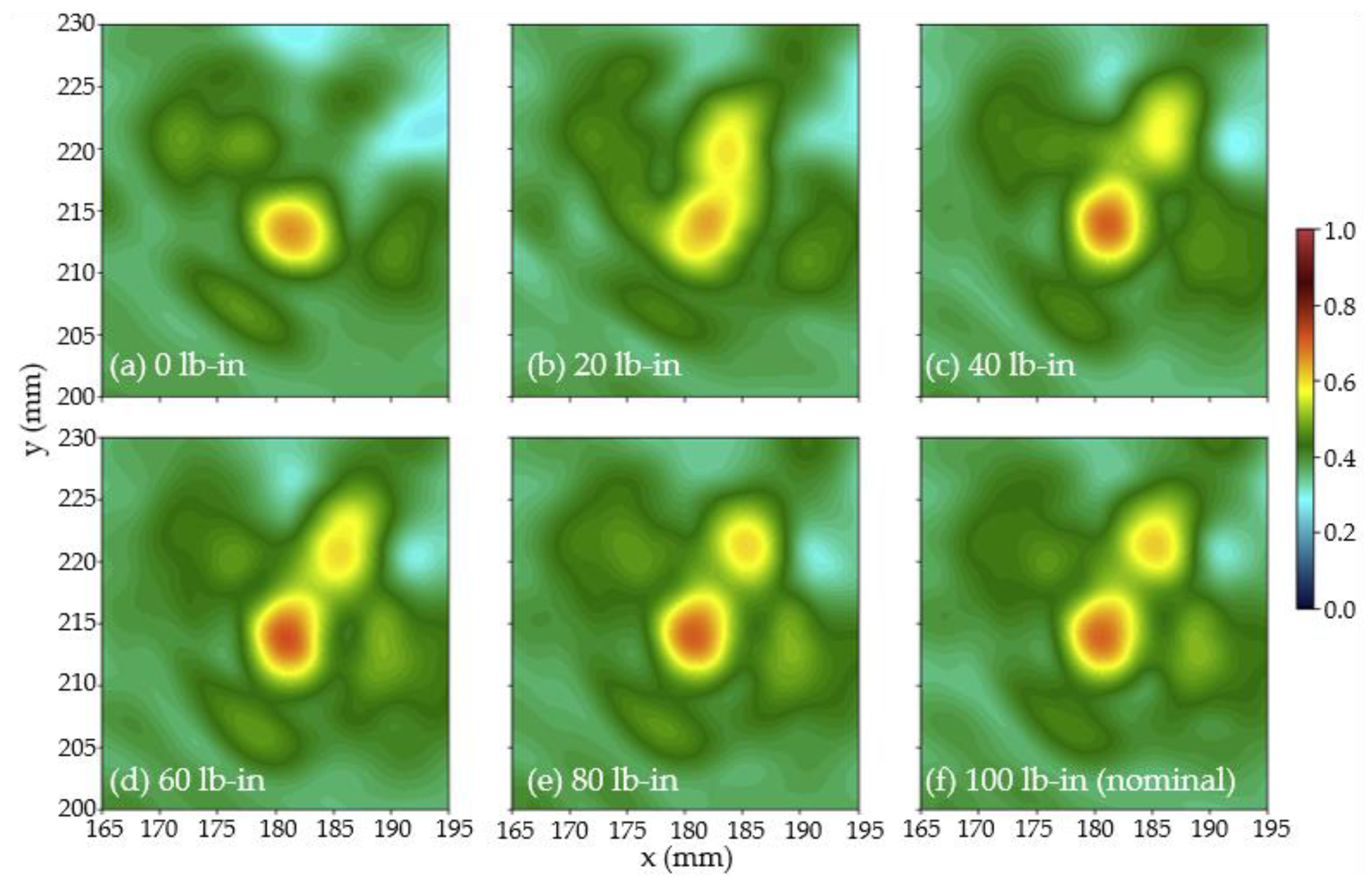
| Inspection Sequence | 1 | 2 | 3 | 4 | 5 | 6 | |
|---|---|---|---|---|---|---|---|
| Torque level | (lb-in) | 0 | 20 | 40 | 60 | 80 | 100 |
| (Nm) | 0.00 | 2.26 | 4.52 | 6.78 | 9.04 | 11.30 | |
Disclaimer/Publisher’s Note: The statements, opinions and data contained in all publications are solely those of the individual author(s) and contributor(s) and not of MDPI and/or the editor(s). MDPI and/or the editor(s) disclaim responsibility for any injury to people or property resulting from any ideas, methods, instructions or products referred to in the content. |
© 2024 by the authors. Licensee MDPI, Basel, Switzerland. This article is an open access article distributed under the terms and conditions of the Creative Commons Attribution (CC BY) license (https://creativecommons.org/licenses/by/4.0/).
Share and Cite
Yn, L.S.; Romli, F.I.; Mazlan, N.; Lee, J.-R.; Harmin, M.Y.; Ciang, C.C. High-Resolution Wavenumber Bandpass Filtering of Guided Ultrasonic Wavefield for the Visualization of Subtle Structural Flaws. Aerospace 2024, 11, 524. https://doi.org/10.3390/aerospace11070524
Yn LS, Romli FI, Mazlan N, Lee J-R, Harmin MY, Ciang CC. High-Resolution Wavenumber Bandpass Filtering of Guided Ultrasonic Wavefield for the Visualization of Subtle Structural Flaws. Aerospace. 2024; 11(7):524. https://doi.org/10.3390/aerospace11070524
Chicago/Turabian StyleYn, Lee Shi, Fairuz Izzuddin Romli, Norkhairunnisa Mazlan, Jung-Ryul Lee, Mohammad Yazdi Harmin, and Chia Chen Ciang. 2024. "High-Resolution Wavenumber Bandpass Filtering of Guided Ultrasonic Wavefield for the Visualization of Subtle Structural Flaws" Aerospace 11, no. 7: 524. https://doi.org/10.3390/aerospace11070524