

Inter-Satellite Link Prediction with Supervised Learning: An Application in Polar Orbits

Abstract
1. Introduction
2. Encounter Anticipation Problem
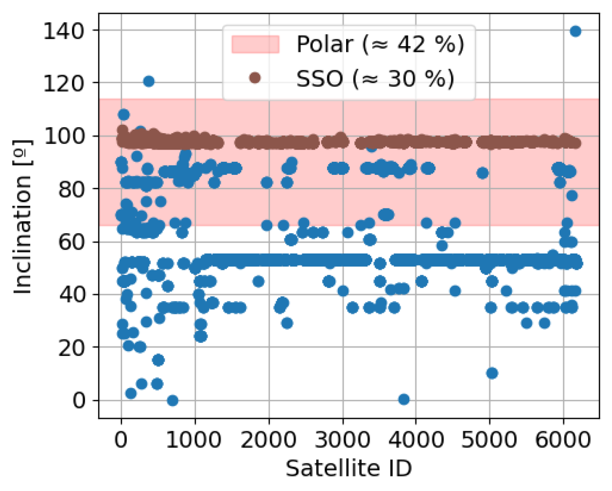
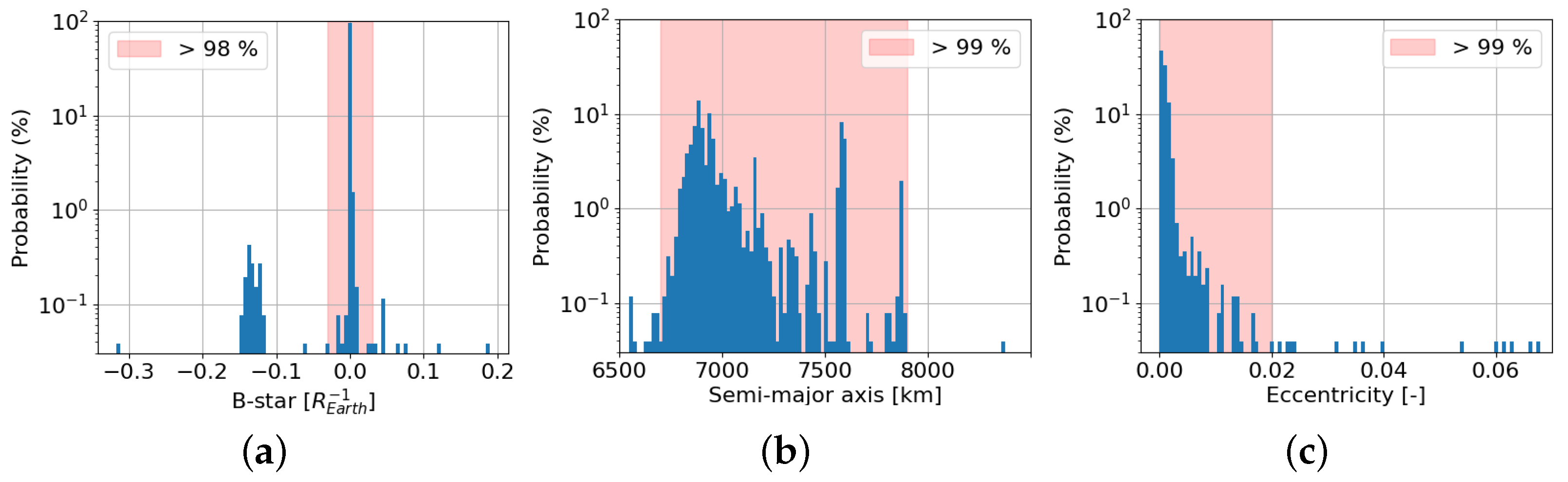
3. Polar Orbits
4. Supervised Learning Model
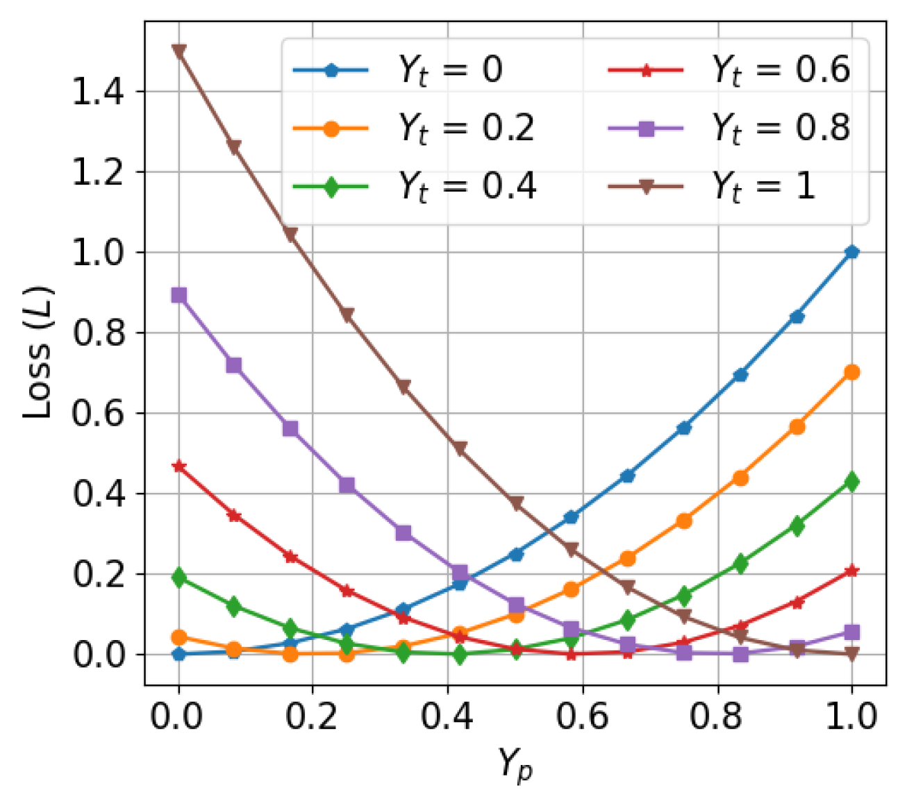
Weighted Loss Function
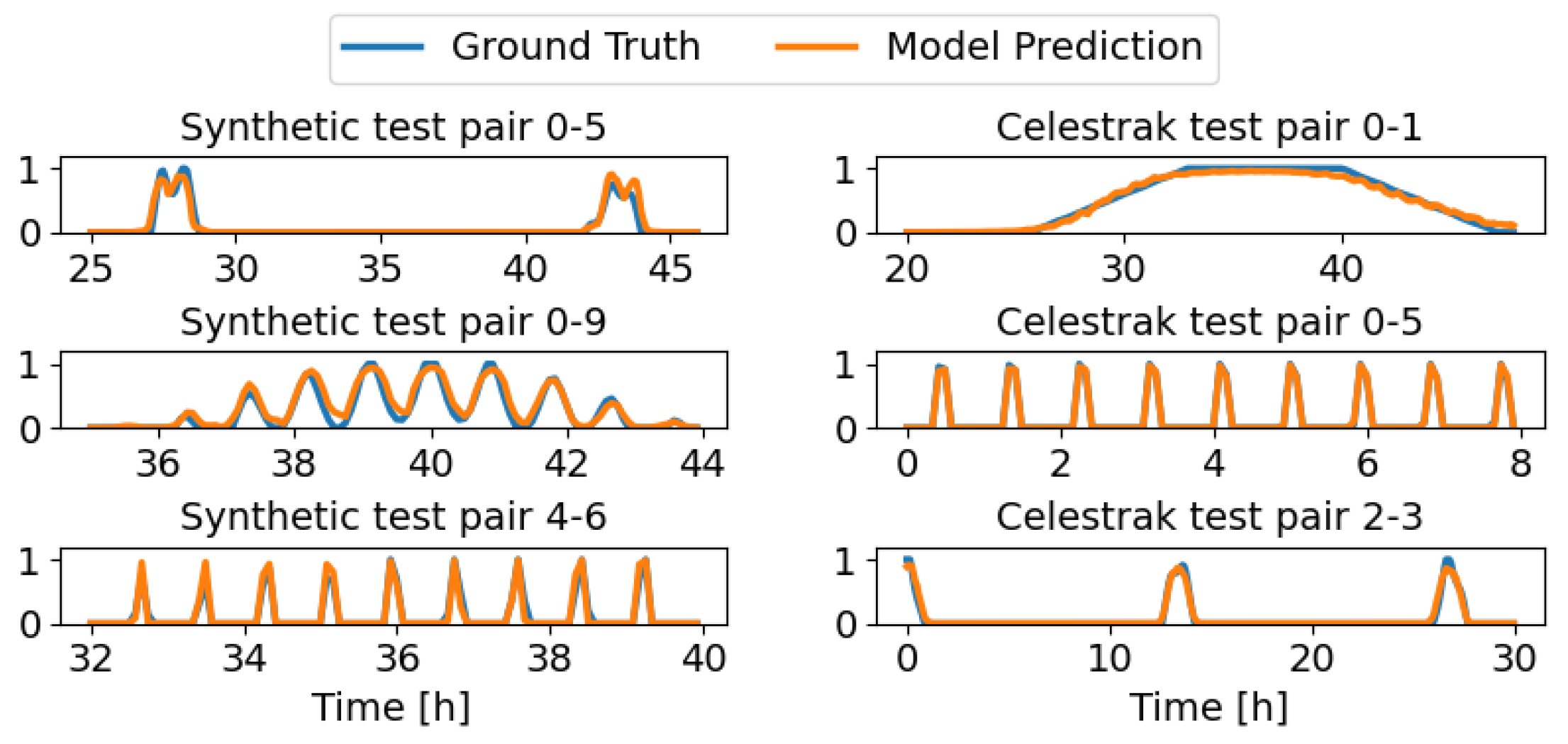
5. Results
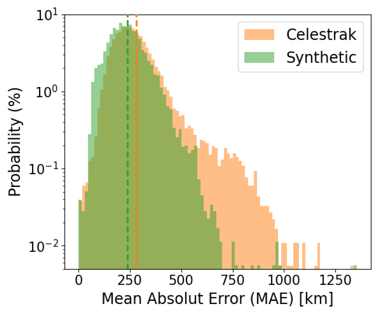
5.1. Distance Error
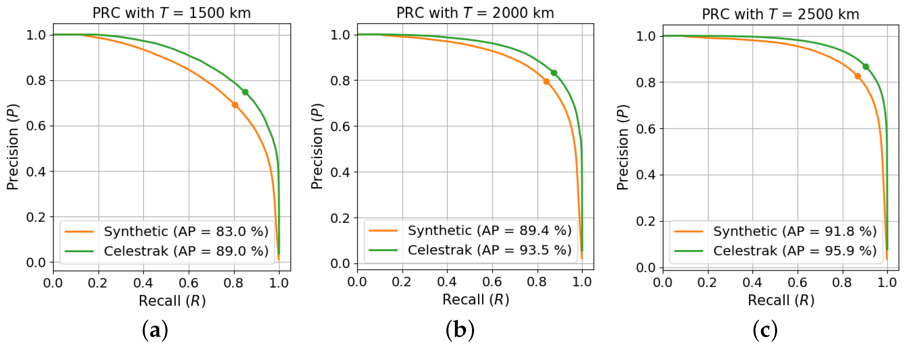
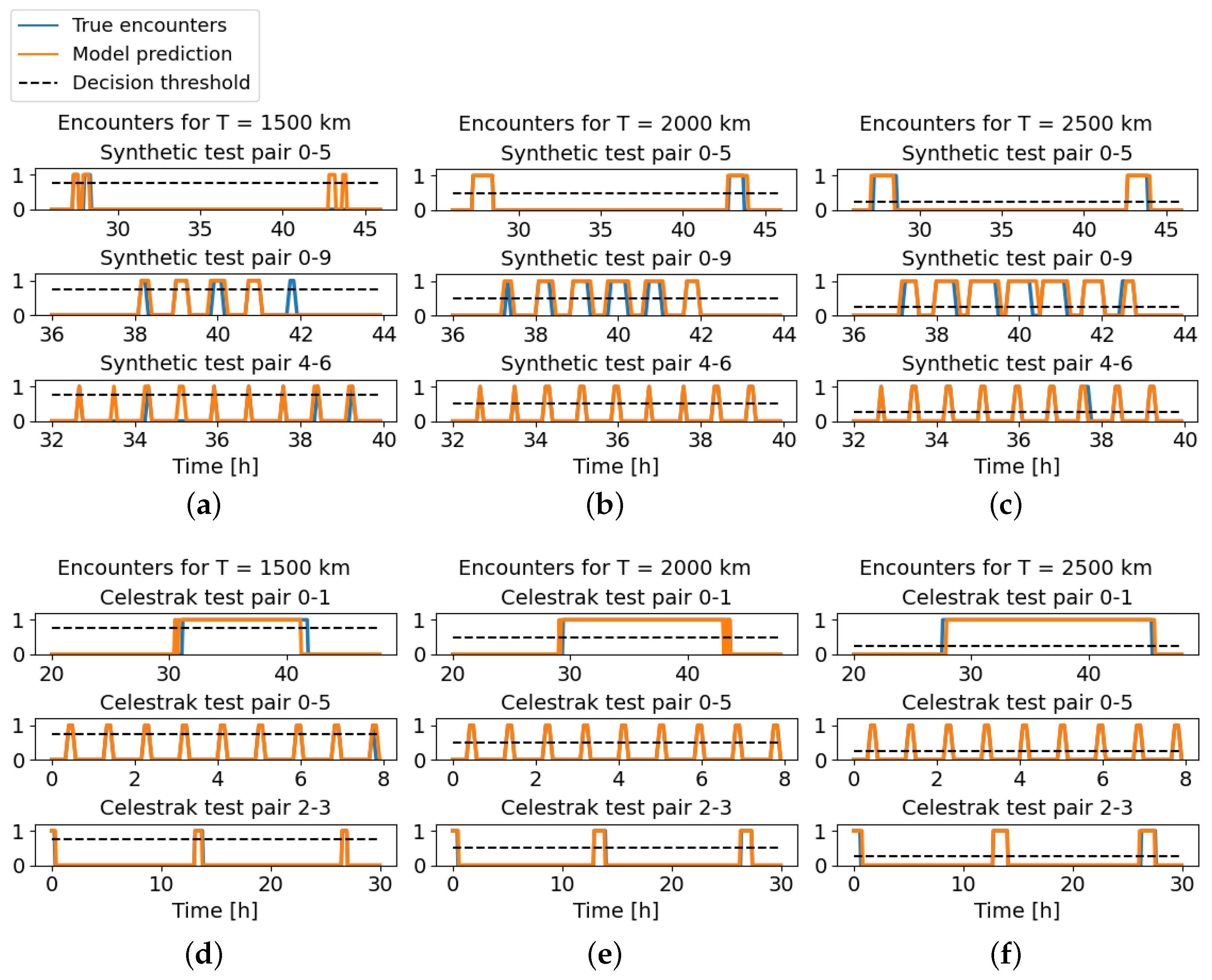
5.2. Fixed Distance Threshold
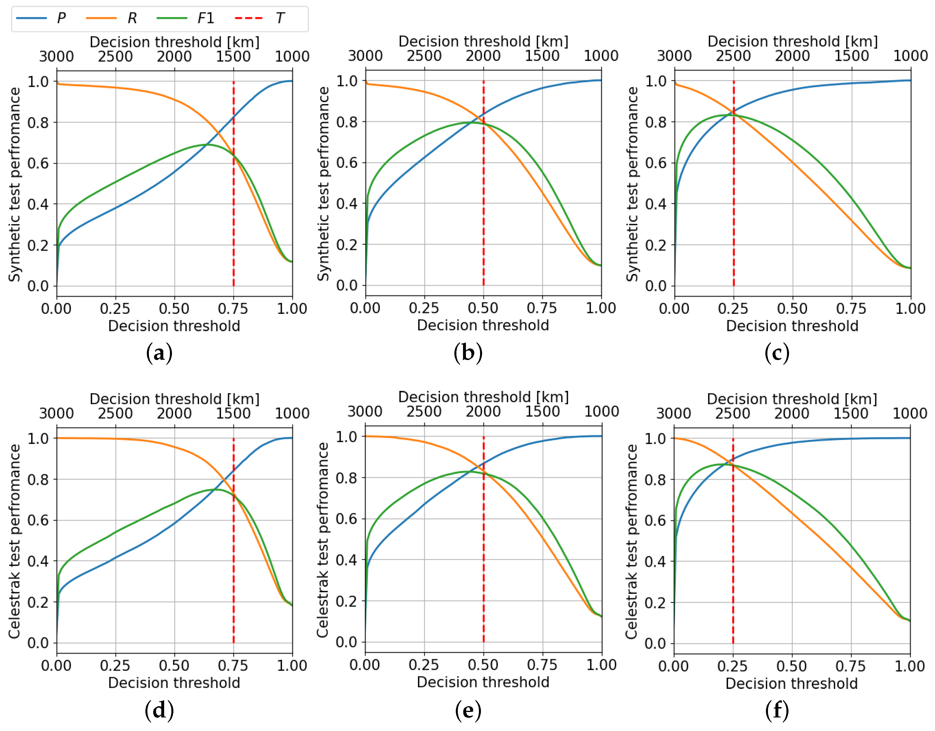
5.3. Fixed Decision Threshold
5.4. Computational Cost
6. Conclusions
Author Contributions
Funding
Institutional Review Board Statement
Data Availability Statement
Conflicts of Interest
Abbreviations
| DSS | Distributed Space Systems |
| ISL | Inter-Satellite Link |
| LEO | Low-Earth Orbit |
| NTN | Non-Terrestrial Network |
| TLE | Two-Line Elements |
| SL | Supervised Learning |
| SGP4 | Simplified General Perturbation 4 |
| T | Distance threshold |
| SSO | Sun-synchronous orbit |
| OE | Orbital Elements |
| MAE | Mean Absolute Error |
| P | Precision |
| R | Recall |
| F1 score | |
| True Positive | |
| False Positive | |
| False Negative | |
| Balance Accuracy | |
| True Negative Rate | |
| AP | Average Precision |
| PRC | Precision-Recall Cruve |
References
- Araguz, C. In pursuit of Autonomous Distributed Satellite Systems. Ph.D. Thesis, Polytechnic University of Catalonia, Barcelona, Spain, 2019. [Google Scholar]
- Giordani, M.; Zorzi, M. Non-terrestrial networks in the 6G era: Challenges and opportunities. IEEE Netw. 2020, 35, 244–251. [Google Scholar] [CrossRef]
- Ben-Larbi, M.K.; Pozo, K.F.; Haylok, T.; Choi, M.; Grzesik, B.; Haas, A.; Krupke, D.; Konstanski, H.; Schaus, V.; Fekete, S.P.; et al. Towards the automated operations of large distributed satellite systems. Part 1: Review and paradigm shifts. Adv. Space Res. 2021, 67, 3598–3619. [Google Scholar] [CrossRef]
- Ben-Larbi, M.K.; Pozo, K.F.; Choi, M.; Haylok, T.; Grzesik, B.; Haas, A.; Krupke, D.; Konstanski, H.; Schaus, V.; Fekete, S.P.; et al. Towards the automated operations of large distributed satellite systems. Part 2: Classifications and tools. Adv. Space Res. 2021, 67, 3620–3637. [Google Scholar] [CrossRef]
- Fraire, J.A.; Finochietto, J.M. Design challenges in contact plans for disruption-tolerant satellite networks. IEEE Commun. Mag. 2015, 53, 163–169. [Google Scholar] [CrossRef]
- de Azúa, J.A.R.; Calveras, A.; Camps, A. Internet of satellites (IoSat): Analysis of network models and routing protocol requirements. IEEE Access 2018, 6, 20390–20411. [Google Scholar] [CrossRef]
- Du, B.; Li, S. A new multi-satellite autonomous mission allocation and planning method. Acta Astronaut. 2019, 163, 287–298. [Google Scholar] [CrossRef]
- Yao, F.; Li, J.; Chen, Y.; Chu, X.; Zhao, B. Task allocation strategies for cooperative task planning of multi-autonomous satellite constellation. Adv. Space Res. 2019, 63, 1073–1084. [Google Scholar] [CrossRef]
- Fossa, C.E.; Raines, R.A.; Gunsch, G.H.; Temple, M.A. An overview of the IRIDIUM (R) low Earth orbit (LEO) satellite system. In Proceedings of the IEEE 1998 National Aerospace and Electronics Conference. NAECON 1998. Celebrating 50 Years (Cat. No. 98CH36185), Dayton, OH, USA, 17 July 1998; IEEE: Piscataway, NJ, USA, 1998; pp. 152–159. [Google Scholar]
- Walker, J.G. Satellite constellations. J. Br. Interplanet. Soc. 1984, 37, 559. [Google Scholar]
- Fischer, D.; Basin, D.; Eckstein, K.; Engel, T. Predictable mobile routing for spacecraft networks. IEEE Trans. Mob. Comput. 2012, 12, 1174–1187. [Google Scholar] [CrossRef]
- Su, W.; Malaer, J.; Cho, O.; Suh, K. Using mobility prediction to enhance network routing in LEO crosslink network. In Proceedings of the International Astronautical Congress (IAC 2019), Washington, DC, USA, 21–25 October 2019. [Google Scholar]
- Ruiz-De-Azua, J.A.; Ramírez, V.; Park, H.; AUG, A.C.; Camps, A. Assessment of satellite contacts using predictive algorithms for autonomous satellite networks. IEEE Access 2020, 8, 100732–100748. [Google Scholar] [CrossRef]
- Casadesus, G.; Alarcón, E. Toward autonomous cooperation in heterogeneous nanosatellite constellations using dynamic graph neural networks. In Proceedings of the International Astronautical Congress (IAC 2023), Baku, Azerbaijan, 2–6 October 2023. [Google Scholar]
- Ferrer, E.; Escrig, J.; Ruiz-de Azua, J.A. Inter-Satellite Link Prediction for Non-Terrestrial Networks Using Supervised Learning. In Proceedings of the 2023 Joint European Conference on Networks and Communications & 6G Summit (EuCNC/6G Summit), Gothenburg, Sweden, 6–9 June 2023; IEEE: Piscataway, NJ, USA, 2023; pp. 258–263. [Google Scholar]
- Ferrer, E.; Ruiz-De-Azua, J.A.; Betorz, F.; Escrig, J. Inter-Satellite Link Prediction with Supervised Learning Based on Kepler and SGP4 Orbits. In Artificial Intelligence Research and Development: Proceedings of the 25th International Conference of the Catalan Association for Artificial Intelligence; IOS Press: Amsterdam, The Netherlands, 2023; Volume 375, p. 7. [Google Scholar]
- Hoots, F.R.; Roehrich, R.L. Models for Propagation of NORAD Element Sets; Office of Astrodynamics: Colorado Springs, CO, USA, 1988. [Google Scholar]
- Vallado, D.; Crawford, P. SGP4 orbit determination. In Proceedings of the AIAA/AAS Astrodynamics Specialist Conference and Exhibit, Honolulu, HI, USA, 18–21 August 200; p. 6770.
- Kelso, D.T. Celestrak. 1985. Available online: https://celestrak.org/ (accessed on 16 January 2023).
- Ruiz-de Azua, J.A.; Fernandez, L.; Muñoz, J.F.; Badia, M.; Castella, R.; Diez, C.; Aguilella, A.; Briatore, S.; Garzaniti, N.; Calveras, A.; et al. Proof-of-concept of a federated satellite system between two 6-unit CubeSats for distributed earth observation satellite systems. In Proceedings of the IGARSS 2019—2019 IEEE International Geoscience and Remote Sensing Symposium, Yokohama, Japan, 28 July–2 August 2019; IEEE: Piscataway, NJ, USA, 2019; pp. 8871–8874. [Google Scholar]
- Vallado, D.A.; Cefola, P.J. Two-line element sets–practice and use. In Proceedings of the 63rd International Astronautical Congress, Naples, Italy, –5 October 2012; pp. 1–14. [Google Scholar]
- Wang, Z.; Bovik, A.C. Mean squared error: Love it or leave it? A new look at signal fidelity measures. IEEE Signal Process. Mag. 2009, 26, 98–117. [Google Scholar] [CrossRef]
- Chai, T.; Draxler, R.R. Root mean square error (RMSE) or mean absolute error (MAE). Geosci. Model Dev. Discuss. 2014, 7, 1525–1534. [Google Scholar]
- Mannor, S.; Peleg, D.; Rubinstein, R. The cross entropy method for classification. In Proceedings of the 22nd International Conference on Machine Learning, Bonn, Germany, 7–11 August 2005; pp. 561–568. [Google Scholar]


| Value | [] | a [km] | e [-] | i [°] | [°] | [°] | M [°] |
|---|---|---|---|---|---|---|---|
| From | −0.03 | 6700 | 0 | 66 | 0 | 0 | 0 |
| To | 0.03 | 7900 | 0.02 | 114 | 360 | 360 | 360 |
| T = 1500 km | T = 2000 km | T = 2500 km | ||||
|---|---|---|---|---|---|---|
| TestS | TestC | TestS | TestC | TestS | TestC | |
| [%] | 81.8 | 86.3 | 89.6 | 91.2 | 91.8 | 93.1 |
| [%] | 63.6 | 71.8 | 78.7 | 81.8 | 83.0 | 86.7 |
| P [%] | 82.3 | 83.8 | 83.5 | 86.7 | 84.9 | 89.7 |
| R [%] | 63.8 | 73.2 | 79.6 | 83.1 | 84.2 | 87.0 |
| [%] | 83.0 | 89.0 | 89.4 | 93.5 | 91.8 | 95.9 |
| T = 1500 km | T = 2000 km | T = 2500 km | ||||
|---|---|---|---|---|---|---|
| TestS | TestC | TestS | TestC | TestS | TestC | |
| – | −0.3% | 0.0% | 0.5% | 0.3% | 1.1% | 0.9% |
| – | 1.1% | 1.0% | 1.9% | 1.2% | 1.8% | 1.5% |
| P– | 4.9% | 3.1% | 3.1% | 2.1% | 1.1% | 1.1% |
| R– | −0.8% | −0.3% | 0.9% | 0.5% | 2.1% | 1.6% |
| – | 2.8% | 1.8% | 2.2% | 1.4% | 1.6% | 1.1% |
| TF | TF Lite | SGP4 | |
|---|---|---|---|
| Time [s] | ≈60,000 | ≈70 | ≈420 |
Disclaimer/Publisher’s Note: The statements, opinions and data contained in all publications are solely those of the individual author(s) and contributor(s) and not of MDPI and/or the editor(s). MDPI and/or the editor(s) disclaim responsibility for any injury to people or property resulting from any ideas, methods, instructions or products referred to in the content. |
© 2024 by the authors. Licensee MDPI, Basel, Switzerland. This article is an open access article distributed under the terms and conditions of the Creative Commons Attribution (CC BY) license (https://creativecommons.org/licenses/by/4.0/).
Share and Cite
Ferrer, E.; Ruiz-De-Azua, J.A.; Betorz, F.; Escrig, J. Inter-Satellite Link Prediction with Supervised Learning: An Application in Polar Orbits. Aerospace 2024, 11, 551. https://doi.org/10.3390/aerospace11070551
Ferrer E, Ruiz-De-Azua JA, Betorz F, Escrig J. Inter-Satellite Link Prediction with Supervised Learning: An Application in Polar Orbits. Aerospace. 2024; 11(7):551. https://doi.org/10.3390/aerospace11070551
Chicago/Turabian StyleFerrer, Estel, Joan A. Ruiz-De-Azua, Francesc Betorz, and Josep Escrig. 2024. "Inter-Satellite Link Prediction with Supervised Learning: An Application in Polar Orbits" Aerospace 11, no. 7: 551. https://doi.org/10.3390/aerospace11070551
APA StyleFerrer, E., Ruiz-De-Azua, J. A., Betorz, F., & Escrig, J. (2024). Inter-Satellite Link Prediction with Supervised Learning: An Application in Polar Orbits. Aerospace, 11(7), 551. https://doi.org/10.3390/aerospace11070551