Compound Control Design of Near-Space Hypersonic Vehicle Based on a Time-Varying Linear Quadratic Regulator and Sliding Mode Method

Abstract

The design of a hypersonic vehicle controller has been an active research field in the last decade, especially when the vehicle is studied as a time-varying system. A time-varying compound control method is proposed for a hypersonic vehicle controlled by the direct lateral force and the aerodynamic force. The compound control method consists of a time-varying linear quadratic regulator (LQR) control law for the aerodynamic rudder and a sliding mode control law for the lateral thrusters. When the air rudder cannot continuously produce control force and torque, the direct lateral force is added to the system. To solve the problem that LQR cannot directly obtain the analytical solution of the time-varying system, a novel approach to approximate analytical solutions using Jacobi polynomials is proposed in this paper. Finally, the stability of the time-varying compound control system is proven by the Lyapunov–Krasovskii functional (LKF). The simulation results show that the proposed compound control method is effective and can improve the fast response ability of the system.

1. Introduction

The near-space hypersonic vehicle is a new type of aircraft with a large flight envelope and ultra-high speed that has the advantages of fast response and high penetration success rate. At the same time, the response speed of the tracking acceleration command is also required in the course of combat. Therefore, it has been very important to study the design of the aircraft controller. Due to the influence of thermal protection, lift–drag ratio, aerodynamic rudder size, and other factors of the aircraft, the variation of the deflection angle of the control surfaces is limited within the allowable value range [1]. And it is difficult for the single aerodynamic rudder to continuously and efficiently produce the control force and control torque, which makes it easy to induce the saturation phenomenon [2]. It can be seen that the method based on the command control of direct lateral force and aerodynamic force is an important solution to achieve a fast response of a hypersonic vehicle. In addition, the aerodynamic parameters of the vehicle are constantly changing during the flight [3]. So, the control system of a hypersonic vehicle is time-varying. Because of the complexity of the time-varying system and the variability of the parameters, the control methods of time-invariant systems are limited and not strict when applied to the time-varying system. Therefore, it is particularly important to establish an appropriate time-varying model and design an appropriate control method for it.

The design of a compound control law for a dual controlled hypersonic vehicle has been an important topic. Many researchers at home and abroad have done some research on the compound control method of hypersonic vehicles, including adaptive and sliding mode control [4,5,6,7], LQR and sliding mode control [8,9], neural networks and adaptive control [10,11], active disturbance rejection and sliding mode control [12,13], adaptive and backstepping control [14], sliding mode and PID control [15], etc. However, many of the references are similar to the research methods mentioned above, which are based on the time-invariant system model. In this paper, the design of a compound controller based on time-varying model is proposed.

Currently, there are few relevant publications on the design of time-varying compound controllers for hypersonic vehicles. In [16], although the control object is a time-varying compound control aircraft, it only studies the switching conditions of compound control and does not focus on the design of the compound control law. In [17,18], the compound control of a variable parameter system is studied, but the control process is implemented in stages. Reference [19] uses LQR and a sliding mode control method to design the time-varying control law, but it does not give the solution process of the time-varying control law; that is, it does not get the analytical solution of the LQR method. In this paper, based on a designed time-varying compound control system, a novel method of solving LQR analytical solutions using Jacobi polynomials is presented.

Some scholars have given different methods for the solution of the LQR time-varying control law. Among them, references [20,21,22] use an iterative algorithm to approximately solve the LQR time-varying control law. However, this method is limited by the number of iterations. In [23,24], the LQR control law in a time-varying system is approximately solved by reducing the order of the system state equation, but the stability of the system is affected. In [25], the LQR time-varying control law is solved by using a genetic algorithm, but this method has a strong dependence on the initial conditions. Therefore, herein Jacobi polynomials are proposed to solve the analytical solution of the time-varying LQR.

As for the stability analysis of systems, there are many theories of the stability analysis of time-invariant systems [26,27,28] and also the stability analysis of discrete systems [29,30,31], while the stability analysis of time-varying systems is relatively rare. Based on references [32,33], this paper proposes to study the stability of time-varying control systems by using the Lyapunov–Krasovskii functional (LKF) theory. Compared with time-invariant systems, the stability of time-varying systems is more difficult to deal with because the function describing the dynamics takes time as the parameter. And the theory of inverse Lyapunov is generally not sufficient for studying time-varying systems because such Lyapunov functions are difficult to obtain. Therefore, LKF is used to prove the stability of the designed time-varying system.

In this study, the main contributions are as follows: (1) To solve the problem of time-varying aerodynamic parameters of hypersonic vehicles with direct lateral force and aerodynamic force control during flight, a new time-varying compound control method based on LQR and sliding mode control is proposed. In the aerodynamic control system, the time-varying control law is designed based on LQR. When the air rudder cannot continuously produce control force and torque, the direct lateral force is added to the system. A sliding mode control design method for a time-varying system with direct lateral force control is presented. Compared with the traditional compound control method, this method embodies the time-varying characteristic of the control system and has practical significance. Moreover, the response speed of the system designed by using this method is faster than that of the time-invariant system. (2) The approximate analytical solution of time-varying LQR is derived by using the Jacobi polynomial innovatively. The problem of a difficult analytical solution for time-varying systems is further studied. Compared with the control method of time-invariant systems, it has more practical significance. (3) A novel method is presented to prove the stability of a time-varying compound control system by using the LKF theory.

The structure of this article is as follows. In Section 2, the time-varying model of a hypersonic vehicle is described. In Section 3, the derivation of the approximate analytical solution of the time-varying LQR by using Jacobi polynomials is given. In Section 4, the compound control law based on time-varying LQR and sliding mode theory is designed. The stability analysis of the system based on LKF is proven in Section 5. Simulation results and analyses are illustrated in Section 6. Conclusions are made in Section 7.

2. Dynamic Model

For a compound control hypersonic vehicle in near space, the control torque is generated by both rudders and reaction control systems. Since the aerodynamic parameters change during the flight, it is necessary to establish a time-varying model for the design and analysis. For the skid-to-turn (STT) vehicle, its dynamics model can be decoupled and linearized into a longitudinal channel model, a lateral channel model, and a rolling channel model. The control laws for the three channels can be designed, respectively.

Herein, the longitudinal channel is taken as an example to design the time-varying compound control law. The model can be described as:

$$\left\{\begin{array}{l}{\dot{n}}_y=-a_4(t)n_y+\frac{V}{g}{a}_4(t){\omega }_z-\frac{V}{g}{a}_5{\tau }_1{\delta }_z-\frac{V}{g}{k}_y{\tau }_2{F}_{Ty}+\frac{V}{g}{a}_5{\tau }_1{\delta }_{zc}+\frac{V}{g}{k}_y{\tau }_2{F}_{Tyc}\\ {\dot{\omega }}_z=-a_1{\omega }_z-\frac{a_2(t)g}{a_4(t)V}{n}_y+\left(\frac{a_2(t)a_5}{a_4(t)}-a_3\right){\delta }_z+\left(\frac{a_2(t)k_y}{a_4(t)}-l_z\right)F_{Ty} \\ {\dot{\delta }}_z=-{\tau }_1{\delta }_z+{\tau }_1{\delta }_{zc}\\ {\dot{F}}_{Ty}=-{\tau }_2{F}_{Ty}+{\tau }_2{F}_{Tyc}\end{array}\right.$$

(1)

where $n_y$ is the normal acceleration; $g$ is the gravitational acceleration constant; ${\omega }_z$ is the angular velocity; ${\delta }_z$ is the elevator deflection angle; ${\tau }_1$ and ${\tau }_2$ represent the time constants of the rudder and the direct lateral force, respectively; and $m$ and $V$ are the vehicle mass and flight speed, respectively. $k_y=1/(mV)$; $l_z=-l/J_z$. $l$ represents the distance from the center of force to the center of mass, $J_z$ represents the moment inertia, $F_{Ty}$ represents the direct lateral thrust provided by the engine, $F_{Tyc}$ represents the direct lateral thrust command, and ${\delta }_{zc}$ represents the command of the elevator deflection angle. $a_1$, $a_2$, $a_3$, $a_4$, and $a_5$ are the dynamic coefficients of the hypersonic vehicle, $a_1=-M_z^{{\omega }_z}/J_z$, $a_3=-M_z^{{\delta }_z}/J_z$, $a_5=Y^{{\delta }_z}/(mV)$; the changes in $a_2$ and $a_4$ are expressed as time functions, denoted as $a_2(t)$ and $a_4(t)$. $M_z^{{\omega }_z}$ and $M_z^{{\delta }_z}$ represent the partial derivatives of pitching moment $M_z$ to ${\omega }_z$ and ${\delta }_z$, respectively; $Y^{{\delta }_z}$ represents the partial derivatives of lift $Y$ to ${\delta }_z$.

The tracking error of the normal acceleration command is defined as:

$$e_y=n_{yc}-n_y$$

(2)

where $n_{yc}$ is the normal acceleration command. To improve the tracking accuracy of $n_y$, a tracking error integral term is introduced. Equations (1) and (2) are expressed in state equations. Define the state vectors as $x_1={\displaystyle {\int }_0^t{e}_{y}dt}$, $x_2=e_y$, $x_3={\omega }_z$, $x_4={\delta }_z$, and $x_5=F_{Ty}$, respectively. The control vectors are $u_1={\delta }_{zc}$ and $u_2=F_{Tyc}$, and the state equation is written as

$$\left\{\begin{array}{l}{\dot{x}}_1=x_2\hfill \\ {\dot{x}}_2=-a_4(t)x_2-\frac{V}{g}{a}_4(t)x_3+\frac{V}{g}{a}_5{\tau }_1{x}_4+\frac{V}{g}{k}_y{\tau }_2{x}_5-\frac{V}{g}{a}_5{\tau }_1{u}_1-\frac{V}{g}{k}_y{\tau }_2{u}_2\hfill \\ {\dot{x}}_3=\frac{a_2(t)g}{a_4(t)V}{x}_2-a_1{x}_3+\left(\frac{a_2(t)a_5}{a_4(t)}-a_3\right)x_4+\left(\frac{a_2(t)k_y}{a_4(t)}-l_z\right)x_5\hfill \\ {\dot{x}}_4=-{\tau }_1{x}_4+{\tau }_1{u}_1\hfill \\ {\dot{x}}_5=-{\tau }_2{x}_5+{\tau }_2{u}_2\hfill \end{array}\right.$$

(3)

The design of the compound control law in a time-varying system (3) consists of two parts. The first is that the aerodynamic system controlled by the rudder is studied, and then the system with the direct lateral force is analyzed when the aerodynamic rudder cannot continuously generate control force. When analyzing the aerodynamic control system, the influence of the direct lateral force is ignored; i.e., let $x_5$ and $u_2$ be 0, and the state space equation is expressed as

$${\dot{X}}_1=A_1(t)X_1+B_1{u}_1$$

(4)

In Equation (4), the state vector is $X_1={\left[\begin{array}{cccc}{x}_1& x_2& x_3& x_4\end{array}\right]}^{\mathrm{T}}$, the control vector is $u_1={\delta }_{zc}$, $A_1(t)=\left[\begin{array}{cccc}0& 1& 0& 0\\ 0& -a_4(t)& -\frac{V}{g}{a}_4(t)& \frac{V}{g}{a}_5{\tau }_1\\ 0& \frac{a_2(t)g}{a_4(t)V}& -a_1& \frac{a_2(t)a_5}{a_4(t)}-a_3\\ 0& 0& 0& -{\tau }_1\end{array}\right]$, $B_1=\left[\begin{array}{c}0\\ -\frac{V}{g}{a}_5{\tau }_1\\ 0\\ {\tau }_1\end{array}\right]$.

Since the rank of the controllability matrix of $A_1(t)$ and $B_1$ is 4, the system (4) is completely controllable. And then consider with the linear time-varying control theory, the feedback control law is designed by using LQR. Due to the fact that the analytical solution of time-varying LQR cannot be obtained directly, this paper proposes to obtain the LQR time-varying control law by using Jacobi polynomials.

3. Time-Varying LQR Control Law Design

In this section, in order to solve the time-varying LQR control law, the solution process is derived from the transformation form of the proposed Jacobi polynomials in the time-varying system and its operation matrix.

3.1. The Jacobi Polynomials for Time-Varying System

First, the hypergeometric polynomial is defined as [34]

$$\mathrm{F}(-\tilde{n},\tilde{\beta },\tilde{\gamma },\tilde{z})={\displaystyle \sum _{k=0}^{\tilde{n}}\frac{{(-\tilde{n})}_k{(\tilde{\beta })}_k}{{(\tilde{\gamma })}_{k}k!}}{(\tilde{z})}^k$$

(5)

where $\tilde{z}$ is the variable, the interval is $-1\le \tilde{z}\le 1$; $\tilde{n}$ and $\tilde{\gamma }$ are non-negative integers, and $\tilde{\beta }$ and $k$ are parameters with $\tilde{\beta }>-1$, $k=0,1,\cdots ,\tilde{n}$. The Jacobi polynomials are expressed in the form of hypergeometric polynomials, denoted as $P_{\tilde{n}}^{(\tilde{\alpha },\tilde{\beta })}(\tilde{z})$ [35],

$$\begin{array}{ll}{P}_{\tilde{n}}^{(\tilde{\alpha },\tilde{\beta })}(\tilde{z})& =\frac{{(\tilde{\beta }+1)}_{\tilde{n}}}{\tilde{n}!}\mathrm{F}\left(-\tilde{n},\tilde{n}+\tilde{\alpha }+\tilde{\beta }+1,\tilde{\beta }+1,\frac{1-\tilde{z}}{2}\right)\\ & ={\left(-1\right)}^{\tilde{n}}\frac{{(\tilde{\beta }+1)}_{\tilde{n}}}{\tilde{n}!}\mathrm{F}\left(-\tilde{n},\tilde{n}+\tilde{\alpha }+\tilde{\beta }+1,\tilde{\beta }+1,\frac{1+\tilde{z}}{2}\right)\\ & ={\left(-1\right)}^{\tilde{n}}\frac{{(\tilde{\beta }+1)}_{\tilde{n}}}{\tilde{n}!}{\displaystyle \sum _{k=0}^{\tilde{n}}\frac{{(-\tilde{n})}_k{(\tilde{n}+\tilde{\lambda })}_k}{{(\tilde{\beta }+1)}_{k}k!}}{\left(\frac{1+\tilde{z}}{2}\right)}^k\end{array}$$

(6)

where $\tilde{\alpha }$ is a parameter with $\tilde{\alpha }>-1$, $\tilde{\lambda }=\tilde{\alpha }+\tilde{\beta }+1$; $\tilde{z}\in \left[-1,1\right]$, $(1-\tilde{z})/2\in \left[0,1\right]$, $\frac{1+\tilde{z}}{2}\in \left[0,1\right]$; ${(\tilde{\beta }+1)}_0=1$, ${(\tilde{\beta }+1)}_{\tilde{n}}=\frac{(\tilde{\beta }+\tilde{n})!}{(\tilde{\beta })!}$.

In order to apply the Jacobi polynomials into a time-varying system, it is proposed to convert the variable $\tilde{z}$ to the time variable $t$ with $t\in \left[t_0,t_f\right]$. Due to $\frac{1+\tilde{z}}{2}\in \left[0,1\right]$, $\frac{t-t_0}{t_f-t_0}\in \left[0,1\right]$, let $\frac{1+\tilde{z}}{2}=\frac{t-t_0}{t_f-t_0}$, we can get

$$\tilde{z}=(2t-t_0-t_f)/(t_f-t_0)$$

(7)

The Jacobi polynomials converted to the time-varying system are defined as ${\tilde{J}}_{\tilde{n}}(t)$; ${\tilde{J}}_{\tilde{n}}(t)$ is expressed as

$${\tilde{J}}_{\tilde{n}}(t)=P_{\tilde{n}}^{(\tilde{\alpha },\tilde{\beta })}\left[(2t-t_0-t_f)/(t_f-t_0)\right]=h(\tilde{n}){\displaystyle \sum _{k=0}^{\tilde{n}}\tilde{l}(\tilde{n},k)}{\left(\frac{t-t_0}{t_f-t_0}\right)}^k$$

(8)

where $h(\tilde{n})=\frac{{(-1)}^{\tilde{n}}{(\tilde{\beta }+1)}_{\tilde{n}}}{\tilde{n}!}$ and $\tilde{l}(\tilde{n},k)=\frac{{(-\tilde{n})}_k{(\tilde{n}+\tilde{\lambda })}_k}{k!{(\tilde{\beta }+1)}_k}$. At the same time, the orthogonal property of the Jacobi polynomials is given as:

$${\displaystyle {\int }_{t_0}^{t_f}{(t-t_0)}^{\tilde{\beta }}{(t_f-t)}^{\tilde{\alpha }}{\tilde{J}}_{\tilde{n}}(t)}{\tilde{J}}_j(t)dt=\left\{\begin{array}{ccc}0\hfill & ,\hfill & \tilde{n}\ne j\hfill \\ \frac{{(t_f-t_0)}^{\tilde{\lambda }}}{(2\tilde{n}+\tilde{\lambda })}\cdot \frac{\mathsf{\Gamma }(\tilde{n}+\tilde{\alpha }+1)\mathsf{\Gamma }(\tilde{n}+\tilde{\beta }+1)}{\tilde{n}!\mathsf{\Gamma }(\tilde{n}+\tilde{\lambda })}\hfill & ,\hfill & \tilde{n}=j\hfill \end{array}\right.$$

(9)

where $\mathsf{\Gamma }(\cdot )$ is the Gamma function.

Next, the arbitrary time function $f(t)$ and the arbitrary time matrix $M(t)$ are represented by the Jacobi polynomials, respectively. The arbitrary time function $f(t)$ is denoted by the Jacobi polynomials as:

$$f(t)={\displaystyle \sum _{\tilde{n}=0}^{\tilde{m}-1}{f}_{\tilde{n}}{\tilde{J}}_{\tilde{n}}(t)}=f^T\tilde{J}(t)$$

(10)

where

$$\tilde{J}(t)={[{\tilde{J}}_0(t){\tilde{J}}_1(t) \cdot \cdot \cdot {\tilde{J}}_{\tilde{m}-1}(t)]}^T$$

(11)

$\tilde{J}(t)$ is the Jacobi polynomials vector; $f_{\tilde{n}}$ is the Jacobi polynomials coefficient of $f(t)$; $f={[f_0 f_1 \cdot \cdot \cdot f_{\tilde{m}-1}]}^T$ is the Jacobi polynomials coefficient vector of $f(t)$.

Among them, the Jacobi polynomials coefficient $f_{\tilde{n}}$ can be obtained by solving the minimum value of the integral square error

$$E={\displaystyle {\int }_{t_0}^{t_f}{(t-t_0)}^{\tilde{\beta }}{(t_f-t)}^{\tilde{\alpha }}}{[f(t)-{\displaystyle \sum _{\tilde{n}=0}^{\tilde{m}-1}{f}_{\tilde{n}}{\tilde{J}}_{\tilde{n}}(t)}]}^{2}dt$$

(12)

According to Equation (12), the necessary condition to get the minimum value of $E$ is

$$\frac{\partial E}{\partial f_{\tilde{n}}}=0, \tilde{n}=0,1,\dots ,(\tilde{m}-1)$$

(13)

By the orthogonal property of Equation (9), we can get

$$f_{\tilde{n}}=\tilde{R}(\tilde{n}){\displaystyle {\int }_{t_0}^{t_f}{(t-t_0)}^{\tilde{\beta }}{(t_f-t)}^{\tilde{\alpha }}}f(t){\tilde{J}}_{\tilde{n}}(t)dt$$

(14)

where $\tilde{R}(\tilde{n})=\frac{(2\tilde{n}+\tilde{\lambda })\tilde{n}!\mathsf{\Gamma }(\tilde{n}+\tilde{\lambda })}{{(t_f-t_0)}^{\tilde{\lambda }}\mathsf{\Gamma }(\tilde{n}+\tilde{\alpha }+1)\mathsf{\Gamma }(\tilde{n}+\tilde{\beta }+1)}$.

In addition, the arbitrary time-varying matrix $M(t)$ is expanded by the Jacobi polynomials. For any $\tilde{n}\times \tilde{r}$ dimensional time-varying matrix $M(t)$, it can be expressed as

$$M(t)=\left[\begin{array}{cccc}{m}_{11}(t)& m_{12}(t)& \cdots & m_{1\tilde{r}}(t)\\ m_{21}(t)& m_{22}(t)& \cdots & m_{2\tilde{r}}(t)\\ ⋮& ⋮& \cdots & ⋮\\ m_{\tilde{n}1}(t)& m_{\tilde{n}2}(t)& \cdots & m_{\tilde{n}\tilde{r}}(t)\end{array}\right]$$

(15)

According to Equation (10), the arbitrary time-varying function in the matrix $M(t)$ is represented by the Jacobi polynomials as

$$m_{ij}(t)={\displaystyle \sum _{\tilde{k}=0}^{\tilde{m}-1}{m}_{ij}^{\tilde{k}}{\tilde{J}}_{\tilde{k}}(t)}$$

(16)

where $i$ represents the $i\mathrm{th}$ row of matrix $M(t)$, $i\in \left[1,\tilde{n}\right]$, $j$ represents the $j\mathrm{th}$ column of matrix $M(t)$, $j\in \left[1,\tilde{r}\right]$, $\tilde{k}\in \left[0,\tilde{m}-1\right]$. Then the $M(t)$ can be recorded as

$$M(t)={\displaystyle \sum _{\tilde{k}=0}^{\tilde{m}-1}{M}_{\tilde{k}}{\tilde{J}}_{\tilde{k}}(t)}$$

(17)

with

$$M_{\tilde{k}}=\left[\begin{array}{cccc}{m}_{11}^{\tilde{k}}& m_{12}^{\tilde{k}}& \cdots & m_{1\tilde{r}}^{\tilde{k}}\\ m_{21}^{\tilde{k}}& m_{22}^{\tilde{k}}& \cdots & m_{2\tilde{r}}^{\tilde{k}}\\ ⋮& ⋮& \cdots & ⋮\\ m_{\tilde{n}1}^{\tilde{k}}& m_{\tilde{n}2}^{\tilde{k}}& \cdots & m_{\tilde{n}\tilde{r}}^{\tilde{k}}\end{array}\right]$$

(18)

According to Equation (17), $M(t)$ can be written as

$$M(t)=\left[\begin{array}{cccc}{M}_0& M_1& \cdots & M_{\tilde{m}-1}\end{array}\right]\left[\begin{array}{c}{I}_{\tilde{r}}{\tilde{J}}_0(t)\\ I_{\tilde{r}}{\tilde{J}}_1(t)\\ ⋮\\ I_{\tilde{r}}{\tilde{J}}_{\tilde{m}-1}(t)\end{array}\right]=M{\tilde{J}}_{\tilde{r}}(t)$$

(19)

where $M=\left[\begin{array}{cccc}{M}_0& M_1& \cdots & M_{\tilde{m}-1}\end{array}\right]$, $I_{\tilde{r}}$ represents the $\tilde{r}$ dimensional identity matrix, and ${\tilde{J}}_{\tilde{r}}(t)$ is the generalized Jacobi polynomials vector.

3.2. The Jacobi Polynomials Operation Matrix

In this subsection, the operation matrices of the Jacobi polynomials are further formulated; these include the product operation matrix (POM) and the integral operation matrix (IOM).

To obtain the result of ${\tilde{J}}_{\tilde{n}}(t)\tilde{J}(t)$, according to Equation (11), first, ${\tilde{J}}_{\tilde{n}}(t){\tilde{J}}_j(t)$ is solved, $j\in \left[0,\tilde{m}-1\right]$. Define ${\tilde{g}}_{\tilde{n},j}^{\tilde{k}}$ as the expansion coefficient of ${\tilde{J}}_{\tilde{n}}(t){\tilde{J}}_j(t)$, i.e.,

$${\tilde{J}}_{\tilde{n}}(t){\tilde{J}}_j(t)={\displaystyle \sum _{\tilde{k}=0}^{\tilde{m}-1}{\tilde{g}}_{\tilde{n},j}^{\tilde{k}}{\tilde{J}}_{\tilde{k}}(t)}$$

(20)

Then, according to Equation (14), we can get

$${\tilde{g}}_{\tilde{n},j}^{\tilde{k}}=\tilde{R}(\tilde{k}){\displaystyle {\int }_{t_0}^{t_f}{(t-t_0)}^{\tilde{\beta }}{(t_f-t)}^{\tilde{\alpha }}}{\tilde{J}}_{\tilde{n}}(t){\tilde{J}}_j(t){\tilde{J}}_{\tilde{k}}(t)dt$$

(21)

Combined

$${\displaystyle {\int }_0^1{t}^{\tilde{\beta }}{(1-t)}^{\tilde{\alpha }}}dt=\frac{\mathsf{\Gamma }(\tilde{\beta }+1)\mathsf{\Gamma }(\tilde{\alpha }+1)}{\mathsf{\Gamma }(\tilde{\alpha }+\tilde{\beta }+2)}$$

(22)

and Equation (8), ${\tilde{g}}_{\tilde{n},j}^{\tilde{k}}$ is solved as

$$\begin{array}{ll}{\tilde{g}}_{\tilde{n},j}^{\tilde{k}}& ={(t_f-t_0)}^{\lambda }\tilde{R}(\tilde{k})h(\tilde{n})h(j)h(\tilde{k})\cdot \\ & {\displaystyle \sum _{u=0}^{\tilde{n}}{\displaystyle \sum _{v=0}^j{\displaystyle \sum _{w=0}^{\tilde{k}}\tilde{l}(\tilde{n},u)\tilde{l}}}}(j,v)\tilde{l}(\tilde{k},w)\frac{\mathsf{\Gamma }(u+v+w+\tilde{\beta }+1)\mathsf{\Gamma }(\tilde{\alpha }+1)}{\mathsf{\Gamma }(u+v+w+\tilde{\lambda }+1)}\end{array}$$

(23)

Based on the above process, ${\tilde{J}}_{\tilde{n}}(t)\tilde{J}(t)$ is as follows

$$\begin{array}{ll}{\tilde{J}}_{\tilde{n}}(t)\tilde{J}(t)& ={\left[{\tilde{J}}_{\tilde{n}}(t){\tilde{J}}_0(t){\tilde{J}}_{\tilde{n}}(t){\tilde{J}}_1(t) \cdots {\tilde{J}}_{\tilde{n}}(t){\tilde{J}}_{\tilde{m}-1}(t)\right]}^T\\ & ={\left[\begin{array}{ccc}{\displaystyle \sum _{\tilde{k}=0}^{\tilde{m}-1}{\tilde{g}}_{\tilde{n},0}^{\tilde{k}}{\tilde{J}}_{\tilde{k}}(t)}& {\displaystyle \sum _{\tilde{k}=0}^{\tilde{m}-1}{\tilde{g}}_{\tilde{n},1}^{\tilde{k}}{\tilde{J}}_{\tilde{k}}(t)}\cdot \cdot \cdot & {\displaystyle \sum _{\tilde{k}=0}^{\tilde{m}-1}{\tilde{g}}_{\tilde{n},\tilde{m}-1}^{\tilde{k}}{\tilde{J}}_{\tilde{k}}(t)}\end{array}\right]}^T\\ & =\left[\begin{array}{cccc}{\tilde{g}}_{\tilde{n},0}^0& {\tilde{g}}_{\tilde{n},0}^1& \cdots & {\tilde{g}}_{\tilde{n},0}^{\tilde{m}-1}\\ {\tilde{g}}_{\tilde{n},1}^0& {\tilde{g}}_{\tilde{n},1}^1& \cdots & {\tilde{g}}_{\tilde{n},1}^{\tilde{m}-1}\\ ⋮& ⋮& \cdots & ⋮\\ {\tilde{g}}_{\tilde{n},m^{\prime }-1}^0& {\tilde{g}}_{\tilde{n},\tilde{m}-1}^1& \cdots & {\tilde{g}}_{\tilde{n},\tilde{m}-1}^{\tilde{m}-1}\end{array}\right]\tilde{J}(t)\triangleq G_{\tilde{n}}\tilde{J}(t)\end{array}$$

(24)

where $\tilde{n}\in \left[0,\tilde{m}-1\right]$, $G_{\tilde{n}}$ is the coefficient matrix. Letting $G=\left[G_0 G_1 \cdots G_{\tilde{m}-1}\right]$, $G$ is defined as POM of the Jacobi polynomials. And $G_{\tilde{n}}$ is called the $\tilde{n}\mathrm{th}$ sub-block of $G$.

Furthermore, the integral expression of IOM is performed as the following equation

$${\displaystyle {\int }_{t_0}^{t_f}\tilde{J}(t)}dt=P_{tf}\tilde{J}(t)$$

(25)

where $P_{tf}$ is called the integral operation matrix, shown as follows:

$$P_{tf}=(t_f-t_0)\left[\begin{array}{cccccccc}{\tilde{d}}_0& {\tilde{c}}_1& 0& \cdots & 0& 0& 0& 0\\ {\tilde{d}}_1& {\tilde{b}}_1& {\tilde{c}}_2& \cdots & 0& 0& 0& 0\\ {\tilde{d}}_2& {\tilde{a}}_1& {\tilde{b}}_2& \cdots & 0& 0& 0& 0\\ {\tilde{d}}_3& 0& {\tilde{a}}_2& \cdots & 0& 0& 0& 0\\ ⋮& ⋮& ⋮& & ⋮& ⋮& ⋮& ⋮\\ {\tilde{d}}_{\tilde{m}-3}& 0& 0& \cdots & {\tilde{a}}_{\tilde{m}-4}& {\tilde{b}}_{\tilde{m}-3}& {\tilde{c}}_{\tilde{m}-2}& 0\\ {\tilde{d}}_{\tilde{m}-2}& 0& 0& \cdots & 0& {\tilde{a}}_{\tilde{m}-3}& {\tilde{b}}_{\tilde{m}-2}& {\tilde{c}}_{\tilde{m}-1}\\ {\tilde{d}}_{\tilde{m}-1}& 0& 0& \cdots & 0& 0& {\tilde{a}}_{\tilde{m}-2}& {\tilde{b}}_{\tilde{m}-1}\end{array}\right]$$

(26)

with

• ${\tilde{a}}_{\tilde{i}}=\frac{-(\tilde{\alpha }+\tilde{i}+1)(\tilde{\beta }+\tilde{i}+1)}{(\tilde{\lambda }+2\tilde{i}+2)(\tilde{\lambda }+2\tilde{i}+1)(\tilde{\lambda }+\tilde{i})}$, $(\tilde{i}=1,2,3,\dots ,\tilde{m}-2)$;
• ${\tilde{b}}_{\tilde{i}}=\frac{(\tilde{\alpha }-\tilde{\beta })}{(\tilde{\lambda }+2\tilde{i}+1)(\tilde{\lambda }+2\tilde{i}-1)}$, $(\tilde{i}=1,2,3,\dots ,\tilde{m}-1)$;
• ${\tilde{c}}_{\tilde{i}}=\frac{(\tilde{\lambda }+\tilde{i}-1)}{(\tilde{\lambda }+2\tilde{i}-1)(\tilde{\lambda }+2\tilde{i}-2)}$, $(\tilde{i}=1,2,3,\dots ,\tilde{m}-1)$;
• ${\tilde{d}}_0=\frac{\tilde{\beta }+1}{\tilde{\lambda }+1}$, ${\tilde{d}}_1=-\frac{(\tilde{\beta }+1)(\tilde{\alpha }+1)}{\tilde{\lambda }(\tilde{\lambda }+1)(\tilde{\lambda }+2)}-\frac{\mathsf{\Gamma }(\tilde{\beta }+2)}{2!\tilde{\lambda }\mathsf{\Gamma }(\tilde{\beta })}$,
• ${\tilde{d}}_{\tilde{i}}=\frac{{(-1)}^{\tilde{i}}\mathsf{\Gamma }(\tilde{\beta }+\tilde{i}+1)}{(\tilde{i}+1)!(\tilde{\lambda }+\tilde{i}-1)\mathsf{\Gamma }(\tilde{\beta })}$, $(\tilde{i}=2,3,\dots ,\tilde{m}-1)$.

3.3. LQR Time-Varying Control Law

Based on Section 3.1 and Section 3.2, the LQR time-varying control law is derived. First, consider the following minimum quadratic index [36,37,38]

$${\widehat{J}}_{\min }=\frac{1}{2}{\displaystyle {\int }_{t_0}^{t_f}\left[x^{\mathrm{T}}(t)Q(t)x(t)+\right.}\left.u^T(t)R(t)u(t)\right]dt$$

(27)

For a linear time-varying system

$$\dot{x}(t)=A(t)x(t)+B(t)u(t),t\in [t_0,t_f]$$

(28)

where $Q(t)\ge 0$, $R(t)>0$, $x(t)$ is a $\tilde{n}$ dimensional state vector, $u(t)$ is a $\tilde{r}$ dimensional control vector, and $A(t)$ and $B(t)$ are $\tilde{n}\times \tilde{n}$ dimensional and $\tilde{n}\times \tilde{r}$ dimensional time-varying matrices, respectively. The elements of matrix $A(t)$ and matrix $B(t)$ are continuous functions for the time interval $0\le t_0\le t\le t_f<\infty$. The time-varying control law is

$$u(t)=-R^{-1}(t)B^{\mathrm{T}}(t)P(t)x(t)$$

(29)

Define

$$\lambda (t)=P(t)x(t).$$

(30)

If and only if $\lambda (t)\left|{ }_{t=t_f}\right.=\lambda (t_f)=0$. Then

$$u(t)=-R^{-1}(t)B^{\mathrm{T}}(t)\lambda (t)=-K(t)x(t),t\in [t_0,t_f]$$

(31)

where $K(t)$ is the feedback gain, $K(t)=R^{-1}(t)B^{\mathrm{T}}(t)P(t)$ and $P(t)$ satisfies

$$-\dot{P}(t)=P(t)A(t)+A^{\mathrm{T}}(t)P(t)-P(t)B(t)\times R^{-1}(t)B^{\mathrm{T}}(t)P(t)+Q(t)$$

(32)

The augmented state equation can be written as

$$\left[\begin{array}{c}\dot{x}(t)\\ \dot{\lambda }(t)\end{array}\right]=\left[\begin{array}{cc}A(t)& -B(t)R^{-1}(t)B^{\mathrm{T}}(t)\\ -Q(t)& -A^{\mathrm{T}}(t)\end{array}\right]\left[\begin{array}{c}x(t)\\ \lambda (t)\end{array}\right]=F(t)\left[\begin{array}{c}x(t)\\ \lambda (t)\end{array}\right]$$

(33)

where $F(t)$ is a time-varying matrix. Next, define the state transition matrix of the augmented state Equation (33) as $\Omega (t_0,t_f)=\left[\begin{array}{cc}{\Omega }_{11}(t_0,t_f)& {\Omega }_{12}(t_0,t_f)\\ {\Omega }_{21}(t_0,t_f)& {\Omega }_{22}(t_0,t_f)\end{array}\right]$, $\Omega (t_0,t_f)$ is a $2\tilde{n}\times 2\tilde{n}$ dimensional time-varying matrix, and $\Omega (t_0,t_0)=I_{2\tilde{n}}$. We can get

$$\Omega (t_0,t_f)\left[\begin{array}{c}x(t)\\ \lambda (t)\end{array}\right]=\left[\begin{array}{c}x(t_f)\\ \lambda (t_f)\end{array}\right]=\left[\begin{array}{c}x(t_f)\\ 0\end{array}\right]$$

(34)

and

$${\Omega }_{21}(t_0,t_f)x(t)+{\Omega }_{22}(t_0,t_f)\lambda (t)=\lambda (t_f)=0$$

(35)

Further,

$$\lambda (t)=-{\left[{\Omega }_{22}(t_0,t_f)\right]}^{-1}\left[{\Omega }_{21}(t_0,t_f)\right]x(t)$$

(36)

$P(t)$ can be described as [39]

$$P(t)=-{\left[{\Omega }_{22}(t_0,t_f)\right]}^{-1}\left[{\Omega }_{21}(t_0,t_f)\right]$$

(37)

To determine $P(t)$ and $\Omega (t_0,t_f)$, we take the derivative of Equation (34) and combine it with Equation (33), then the following result is obtained:

$$\dot{\Omega }(t_0,t_f)\left[\begin{array}{c}x(t)\\ \lambda (t)\end{array}\right]=-\Omega (t_0,t_f)\left[\begin{array}{c}\dot{x}(t)\\ \dot{\lambda }(t)\end{array}\right]=-\Omega (t_0,t_f)F(t)\left[\begin{array}{c}x(t)\\ \lambda (t)\end{array}\right]$$

(38)

Therefore,

$$\dot{\Omega }(t_0,t_f)=-\Omega (t_0,t_f)F(t)$$

(39)

To get $u(t)$ in Equation (29), the key is to solve Equation (39). By integrating Equation (39) from $t_0$ to $t_f$, we get

$$\Omega (t_0,t_f)-I_{2\tilde{n}}=-{\displaystyle {\int }_{t_0}^{t_f}\Omega (t_0,t_f)F(t)}dt$$

(40)

According to Equation (19), $\Omega (t_0,t_f)$ and $F(t)$ are expressed by the Jacobi polynomial as

$$F(t)=F{\tilde{J}}_{2\tilde{n}}(t)$$

(41)

$$\Omega (t_0,t_f)=\Omega {\tilde{J}}_{2\tilde{n}}(t)$$

(42)

$$I_{2\tilde{n}}=\left[\begin{array}{cccc}{I}_{2\tilde{n}}& 0& \cdots & 0\end{array}\right]{\tilde{J}}_{2\tilde{n}}(t)$$

(43)

Substituting Equations (41)–(43) into Equation (40), we get

$$\Omega {\tilde{J}}_{2\tilde{n}}(t)=-{\displaystyle {\int }_{t_0}^{t_f}\Omega {\tilde{J}}_{2\tilde{n}}(t)F{\tilde{J}}_{2\tilde{n}}(t)}dt+\left[\begin{array}{cccc}{I}_{2\tilde{n}}& 0& \cdots & 0\end{array}\right]{\tilde{J}}_{2\tilde{n}}(t)$$

(44)

The integral term in Equation (44) can be described as the Kronecker product, i.e.,

$$\Omega {\tilde{J}}_{2\tilde{n}}(t)F{\tilde{J}}_{2\tilde{n}}(t)=\Omega \left[{\displaystyle \sum _{\tilde{k}=0}^{\tilde{m}-1}{G}_{\tilde{k}}\otimes F_{\tilde{k}}}\right]{\tilde{J}}_{2\tilde{n}}(t)$$

(45)

where $G_{\tilde{k}}$ is the $\tilde{k}\mathrm{th}$ sub-block of the product operation matrix according to Equation (24), and $\otimes$ represents the Kronecker product. Herein, the expansion process of Equation (45) is given. The left side of Equation (45) is written in the form of a time-varying matrix polynomial series according to Equations (17), (41) and (42), i.e.,

$$\begin{array}{l}\Omega {\tilde{J}}_{2\tilde{n}}(t)F{\tilde{J}}_{2\tilde{n}}(t)=\left[{\displaystyle \sum _{\tilde{k}=0}^{\tilde{m}-1}{\Omega }_{\tilde{k}}{\tilde{J}}_{\tilde{k}}(t)}\right]\left[{\displaystyle \sum _{\tilde{k}=0}^{\tilde{m}-1}{F}_{\tilde{k}}{\tilde{J}}_{\tilde{k}}(t)}\right]\\ =\left[{\Omega }_0{\tilde{J}}_0(t)+{\Omega }_1{\tilde{J}}_1(t)+\cdots +{\Omega }_{\tilde{m}-1}{\tilde{J}}_{\tilde{m}-1}(t)\right]\left[F_0{\tilde{J}}_0(t)+F_1{\tilde{J}}_1(t)+\cdots +F_{\tilde{m}-1}{\tilde{J}}_{\tilde{m}-1}(t)\right]\end{array}$$

(46)

According to Equations (24), the Equation (46) can be further written as

$$\begin{array}{ll}\Omega {\tilde{J}}_{2\tilde{n}}(t)F{\tilde{J}}_{2\tilde{n}}(t)& =\left[\begin{array}{cccc}{\Omega }_0& {\Omega }_1& \cdots & {\Omega }_{\tilde{m}-1}\end{array}\right]\left[{\displaystyle \sum _{\tilde{k}=0}^{\tilde{m}-1}{G}_{\tilde{k}}\otimes F_{\tilde{k}}}\right]{\left[\begin{array}{cccc}{\tilde{J}}_0& {\tilde{J}}_1& \cdots & {\tilde{J}}_{\tilde{m}-1}\end{array}\right]}^T\\ & =\Omega \left[{\displaystyle \sum _{\tilde{k}=0}^{\tilde{m}-1}{G}_{\tilde{k}}\otimes F_{\tilde{k}}}\right]{\tilde{J}}_{2\tilde{n}}(t)\end{array}$$

(47)

According to Equation (25), it is easy to get

$${\displaystyle {\int }_{t_0}^{t_f}{\tilde{J}}_{2\tilde{n}}(t)}dt=\left(P_{tf}\otimes I_{2\tilde{n}}\right){\tilde{J}}_{2\tilde{n}}(t)$$

(48)

Substituting Equations (45) and (48) into Equation (44), we can get

$$\begin{array}{ll}\Omega {\tilde{J}}_{2\tilde{n}}(t)& =-\Omega \left[{\displaystyle \sum _{\tilde{k}=0}^{\tilde{m}-1}{G}_{\tilde{k}}\otimes F_{\tilde{k}}}\right]{\displaystyle {\int }_{t_0}^{t_f}{\tilde{J}}_{2\tilde{n}}(t)dt+}\left[\begin{array}{cccc}{I}_{2\tilde{n}}& 0& \dots & 0\end{array}\right]{\tilde{J}}_{2\tilde{n}}(t)\\ & =-\Omega \left[{\displaystyle \sum _{\tilde{k}=0}^{\tilde{m}-1}{G}_{\tilde{k}}\otimes F_{\tilde{k}}}\right]\left(P_{tf}\otimes I_{2\tilde{n}}\right){\tilde{J}}_{2\tilde{n}}(t)+\left[\begin{array}{cccc}{I}_{2\tilde{n}}& 0& \dots & 0\end{array}\right]{\tilde{J}}_{2\tilde{n}}(t)\end{array}$$

(49)

Since ${\tilde{J}}_{2\tilde{n}}(t)$ is linearly independent, Equation (49) can be written as

$$\Omega =-\Omega \left[{\displaystyle \sum _{\tilde{k}=0}^{\tilde{m}-1}{G}_{\tilde{k}}\otimes F_{\tilde{k}}}\right]\left(P_{tf}\otimes I_{2\tilde{n}}\right)+\left[\begin{array}{cccc}{I}_{2\tilde{n}}& 0& \dots & 0\end{array}\right]$$

(50)

Further,

$$\Omega =\left[\begin{array}{cccc}{I}_{2\tilde{n}}& 0& \dots & 0\end{array}\right]{\left[\left[\begin{array}{cccc}{I}_{2\tilde{n}}& 0& \dots & 0\end{array}\right]+\left({\displaystyle \sum _{\tilde{k}=0}^{\tilde{m}-1}{G}_{\tilde{k}}\otimes F_{\tilde{k}}}\right)\left(P_{tf}\otimes I_{2\tilde{n}}\right)\right]}^{-1}$$

(51)

Based on the above analysis, $K(t)$ can be obtained according to Equations (29), (37), (42), and (51). The above steps of solving the LQR time-varying control law are organized into a flow chart as shown in Figure 1.

By the above method of solving the time-varying control law, the command of rudder deflection for system (4) is written as

$$u_1=K(t)X_1=K_1(t)x_1+K_2(t)x_2+K_3(t)x_3+K_4(t)x_4$$

(52)

where $K(t)=\left[\begin{array}{cccc}{K}_1(t)& K_2(t)& K_3(t)& K_4(t)\end{array}\right]$. Substituting Equation (52) into system (4), the closed-loop system is written as

$${\dot{X}}_1=(A_1(t)+B_{1}K(t))X_1={\overline{A}}_1(t)X_1$$

(53)

where ${\overline{A}}_1(t)=\left[\begin{array}{cccc}0& 1& 0& 0\\ {\overline{a}}_{21}(t)& {\overline{a}}_{22}(t)& {\overline{a}}_{23}(t)& {\overline{a}}_{24}(t)\\ 0& {\overline{a}}_{32}(t)& -a_1& {\overline{a}}_{34}(t)\\ {\overline{a}}_{41}(t)& {\overline{a}}_{42}(t)& {\overline{a}}_{43}(t)& {\overline{a}}_{44}(t)\end{array}\right]$, with ${\overline{a}}_{21}(t)=-V{a}_5{\tau }_1{K}_1(t)/g$, ${\overline{a}}_{22}(t)=-a_4(t)-V{a}_5{\tau }_1{K}_2(t)/g$, ${\overline{a}}_{23}(t)=-V{a}_4(t)/g-V{a}_5{\tau }_1{K}_3(t)/g$, ${\overline{a}}_{24}(t)=V{a}_5{\tau }_1/g-V{a}_5{\tau }_1{K}_4(t)/g$, ${\overline{a}}_{32}(t)=a_2(t)g/a_4(t)V$, ${\overline{a}}_{34}(t)=a_2(t)a_5/a_4(t)-a_3$, ${\overline{a}}_{41}(t)={\tau }_1{K}_1(t)$, ${\overline{a}}_{42}(t)={\tau }_1{K}_2(t)$, ${\overline{a}}_{43}(t)={\tau }_1{K}_3(t)$, ${\overline{a}}_{44}(t)=-{\tau }_1+{\tau }_1{K}_4(t)$.

4. Sliding Mode Control Law Design

For the dual controlled hypersonic vehicle, the system model with the direct lateral force is written as

$${\dot{X}}_2=A_2(t)X_2+B_2{u}_2$$

(54)

where the state vector is $X_2={\left[\begin{array}{cc}{X}_1^{\mathrm{T}}& x_5\end{array}\right]}^{\mathrm{T}}$, and the control vector is $u_2=F_{Tyc}$; $A_2(t)=\left[\begin{array}{ccccc}0& 1& 0& 0& 0\\ {\overline{a}}_{21}(t)& {\overline{a}}_{22}(t)& {\overline{a}}_{23}(t)& {\overline{a}}_{24}(t)& {\overline{a}}_{25}(t)\\ 0& {\overline{a}}_{32}(t)& -a_1& {\overline{a}}_{34}(t)& {\overline{a}}_{35}(t)\\ {\overline{a}}_{41}(t)& {\overline{a}}_{42}(t)& {\overline{a}}_{43}(t)& {\overline{a}}_{44}(t)& 0\\ 0& 0& 0& 0& -{\tau }_2\end{array}\right]$, with ${\overline{a}}_{25}(t)=\frac{V{k}_y{\tau }_2}{g}$, ${\overline{a}}_{35}(t)=\frac{a_2(t)k_y}{a_4(t)}-l_z$, $B_2={\left[\begin{array}{ccccc}0& -V{k}_y{\tau }_2/g& 0& 0& {\tau }_2\end{array}\right]}^{\mathrm{T}}$. The rank of the controllability matrix of $A_2(t)$ and $B_2$ is 5, so system (54) is completely controllable. Since the direct lateral thrusters work in an on-off mode, the sliding mode control is an appropriate selection for the lateral thrust control law design.

To design the sliding mode surface, the system (54) needs to be converted into the following controllable standard form.

$$\dot{\overline{X}}=A_3(t)\overline{X}+B_3{u}_2$$

(55)

where ${\mathit{A}}_3(t)=\left[\begin{array}{ccccc}0& 1& 0& 0& 0\\ 0& 0& 1& 0& 0\\ 0& 0& 0& 1& 0\\ 0& 0& 0& 0& 1\\ -{\widehat{a}}_0(t)& -{\widehat{a}}_1(t)& -{\widehat{a}}_2(t)& -{\widehat{a}}_3(t)& -{\widehat{a}}_4(t)\end{array}\right]$, ${\mathit{B}}_3={\left[\begin{array}{ccccc}0& 0& 0& 0& 1\end{array}\right]}^{\mathrm{T}}$, ${\widehat{a}}_0(t)$, ${\widehat{a}}_1(t)$, ${\widehat{a}}_2(t)$, ${\widehat{a}}_3(t)$, ${\widehat{a}}_4(t)$ are the variables converted to the standard form; $\overline{X}={\left[\begin{array}{ccccc}{\overline{x}}_1& {\overline{x}}_2& {\overline{x}}_3& {\overline{x}}_4& {\overline{x}}_5\end{array}\right]}^{\mathrm{T}}$ is called the state vector of the controllable state equation; and $\overline{X}\mathbf{=}{\widehat{P}}^{\mathbf{-}\mathbf{1}}(t)X_{\mathbf{2}}$, $\widehat{P}(t)$ is the transformation matrix as follows

$$\widehat{P}(t)=\left[\begin{array}{c}{\widehat{P}}_1\\ {\widehat{P}}_2\\ {\widehat{P}}_3\\ {\widehat{P}}_4\\ {\widehat{P}}_5\end{array}\right]=\left[\begin{array}{c}{\widehat{P}}_1\\ {\widehat{P}}_1{A}_2(t)\\ {\widehat{P}}_1{A_2}^2(t)\\ {\widehat{P}}_1{A_2}^3(t)\\ {\widehat{P}}_1{A_2}^4(t)\end{array}\right]$$

(56)

with ${\widehat{P}}_1=\left[\begin{array}{cccc}0& 0& \cdots & 1\end{array}\right]{\left[\begin{array}{cccc}{B}_2& A_2(t)B_2& \cdots & {A_2}^4(t)B_2\end{array}\right]}^{-1}$.

Then, the sliding mode is designed as

$$S(\overline{X})={\widehat{P}}_1{\overline{x}}_1+{\widehat{P}}_2{\overline{x}}_2+{\widehat{P}}_3{\overline{x}}_3+{\widehat{P}}_4{\overline{x}}_4+{\overline{x}}_5=0$$

(57)

Herein, the selection of ${\widehat{P}}_1$ through ${\widehat{P}}_4$ ensures that the states converge to the origin. To guarantee the reaching condition of the sliding mode,

$$S(\overline{\mathit{X}})\dot{S}(\overline{\mathit{X}})<0$$

(58)

the sliding mode control law is designed as

$$u_2=\left\{\begin{array}{ll}{F}_s,& S(\overline{X})>0\\ -F_s,& S(\overline{X})<0\end{array}\right.$$

(59)

where $F_s$ is the direct lateral force of the side-jet thruster. To eliminate the chattering phenomenon, the controller with boundary layer is designed as

$$u_2=\left\{\begin{array}{ll}{F}_s,& S(\overline{X})>\epsilon \\ 0,& -\epsilon \le S(\overline{X})\le \epsilon \\ -F_s,& S(\overline{X})<-\epsilon \end{array}\right.$$

(60)

In Equation (60), $\epsilon$ represents a small constant that satisfies $\epsilon >0$. For the near-space hypersonic vehicle, the lateral thruster is able to output two amplitudes. If the current state of the system is far away from the sliding surface, the larger amplitude is taken, while if the state of the system is close to the sliding surface, the smaller amplitude is taken. Thus, to meet the need for chattering elimination and fuel savings, the expression of variable structure control is further written as

$$u_2=\left\{\begin{array}{l}{F}_{s1}\hspace{1em}\hspace{0.33em}\hspace{0.33em}S(\overline{X})\ge {\epsilon }_1\\ F_{s2}\hspace{1em}\hspace{0.33em}\hspace{0.33em}{\epsilon }_2\le S(\overline{X})<{\epsilon }_1\\ 0\hspace{1em}\hspace{1em}\hspace{0.33em}-{\epsilon }_2\le S(\overline{X})<{\epsilon }_2\\ -F_{s2}\hspace{1em}-{\epsilon }_1\le S(\overline{X})<-{\epsilon }_2\\ -F_{s1}\hspace{1em}S(\overline{X})<-{\epsilon }_1\end{array}\right.$$

(61)

where $F_{s1}$ is the larger lateral thrust, $F_{s2}$ is the smaller lateral thrust, and ${\epsilon }_1$ and ${\epsilon }_2$ are boundary constants that satisfy ${\epsilon }_1>{\epsilon }_2>0$. In order to improve the durability of the controller, while eliminating chattering and saving fuel, herein, thrust values with large amplitude differences need to be set. At the same time, to reduce the frequent opening or closing of the controller, it is necessary to select a suitable boundary layer range according to the actual situation. The controller is turned on when the chattering is large, and the controller is not turned on when the chattering is small or even within the allowed fluctuation range, so that the control system tends to a steady state.

5. Stability Analysis

5.1. Lyapunov–Krasovskii Functional

The Lyapunov–Krasovskii functional (LKF) is constructed to analyze the stability of time-varying systems according to the following assumptions [32,33].

Assumption 1.

Consider a system $\dot{x}(t)=A(t)x(t)+B(t)u(t)$, there exists a locally Lipschitz continuous functional $\mathrm{V}(t)$, a scalar function $\mu (t)$, two ${\mathit{\kappa }}_{\infty }$ functions ${\mathrm{v}}_i$, $i=1,2$, and a $\mathit{\kappa }$ function $\gamma$ such that

$$\begin{array}{l}{\mathrm{v}}_1(\left|x(t)\right|)\le \mathrm{V}(t)\le {\mathrm{v}}_2(\left|x(t)\right|)\\ \dot{\mathrm{V}}(t)\le \mu (t)\mathrm{V}(t)+\gamma (\left|\mathrm{v}(t)\right|)\end{array}$$

(62)

Consider the following linear time-varying (LTV) system about some concepts of the scalar function $\mu (t)$,

$$\dot{y}(t)=\frac{1}{2}\mu (t)y(t)$$

(63)

where $y(t)$ is the state variable. If there exist two positive constants $k$ and $a$ such that the solution to the scalar system (63) satisfies

$${\left|y(t)\right|}^2\le {\left|y(t_0)\right|}^{2}k{e}^{-a(t-t_0)},t\ge t_0$$

(64)

then the scalar function $\mu (t)$ is said to be uniformly exponentially stable (UES). If there exist two positive constants $k_0$ and $a_0$ such that the solution to the scalar system (63) satisfies

$${\left|y(t)\right|}^2\ge {\left|y(t_0)\right|}^2{k}_0{e}^{-a_0(t-t_0)},t\ge t_0$$

(65)

then the scalar function $\mu (t)$ is said to be uniformly exponentially expanding (UEE). By noting that the solution $y(t)$ to Equation (63) is

$$y(t)=y(t_0)\exp \left(\frac{1}{2}{\displaystyle {\int }_{t_0}^t\mu (s)ds}\right),t\ge t_0$$

(66)

we further conclude that $\mu (t)$ is a UES function if and only if there exist two constants $a>0$ and $b\ge 0$ such that

$${\displaystyle {\int }_{t_0}^t\mu (s)ds}\le -a(t-t_0)+b,t\ge t_0$$

(67)

and $\mu (t)$ is a UEE function if and only if there exist two constants $a_0>0$ and $b_0\in \mathrm{R}$ such that

$${\displaystyle {\int }_{t_0}^t\mu (s)ds}\ge -a_0(t-t_0)+b_0,t\ge t_0$$

(68)

When Equations (67) and (68) are satisfied, $\mu (t)$ is both UES and UEE, where $a_0>a$ and $b\ge b_0$.

We end this subsection with the following lemma.

Lemma 1 

([32,33]). Consider Assumption 1. Let $\mu (t)$ be a both UES and UEE function satisfying Equations (67) and (68), $T_m$ be a constant such that

$$T_m>\frac{nb}{a}.$$

(69)

Then $W_n$ is a LKF for which is defined as

$$W_n(t)\triangleq \mathrm{V}(t)\exp \left({\displaystyle {\int }_t^{t+T_m}\mu (\tau ){\left(1-\frac{\tau -t}{T_m}\right)}^{n}d\tau }\right)$$

(70)

where $n\ge 1$ is a positive constant, $\mathrm{V}(t)$ satisfies Assumption 1. And $W_n(t)$ is written in the following form

$$\begin{array}{l}{k}_n{\mathrm{v}}_1(\left|x(t)\right|)\le W_n(t)\le K_n{\mathrm{v}}_2(\left|x(t)\right|)\\ {\dot{W}}_n(t)\le -{\nu }_n{W}_n(t)+K_n\gamma (\mathrm{v}\left|(t)\right|)\end{array}$$

(71)

where $k_n=e^{-a_0{T}_m/(n+1)+b_0}$, $K_n=e^{-a{T}_m/(n+1)+b}$, and ${\nu }_n=a-nb/T_m>0$.

5.2. Stability Analysis

In order to analyze the stability of the time-varying compound control system, firstly, the parameters of the hypersonic vehicle are given in

Table 1. Parameters of the hypersonic vehicle.

Parameter	Value	Unit
$m$	500	kg
$V$	1963.4	m/s
${\tau }_1$	0.0025	s
${\tau }_2$	0.001	s
$l$	1.36	m
$g$	9.81	m/s2
$J_z$	300	Nms2

.

In the hypersonic vehicle time-varying system, the aerodynamic parameter $a_1=0.0381$, $a_3=14.1014$, and $a_5=0.0062$. $a_2(t)$ is a bounded time-varying parameter, according to the actual situation, and $a_4(t)$ and $a_2(t)$ are approximately proportional, so it is denoted as $a_4(t)=k_a{a}_2(t)$; herein, the proportionality coefficient is taken as $k_a=-0.042$.

According to the method employed by Zhao and Zhou [32,33], the stability analysis of the hypersonic vehicle is given. In system (55), the matrix ${\mathit{A}}_3(t)$ of the standard form system is written as

$${\mathit{A}}_3(t)=\left[\begin{array}{ccccc}0& 1& 0& 0& 0\\ 0& 0& 1& 0& 0\\ 0& 0& 0& 1& 0\\ 0& 0& 0& 0& 1\\ -{\widehat{r}}_0(t)& -{\widehat{r}}_1(t)& -{\widehat{r}}_2(t)& -{\widehat{r}}_3(t)& -{\widehat{r}}_4(t)\end{array}\right],$$

with ${\widehat{r}}_0(t)=-{9.293\mathrm{e}}^{-5}{a}_2(t)-{9.382\mathrm{e}}^5$, ${\widehat{r}}_1(t)=1909a_2(t)+{2.622\mathrm{e}}^7$, ${\widehat{r}}_2(t)=\mathrm{46,200}{a}_2(t)+{3.187\mathrm{e}}^6$, ${\widehat{r}}_3(t)=396.4a_2(t)+{1.605\mathrm{e}}^5$, ${\widehat{r}}_4(t)=-0.09491a_2(t)+1156$. $B_3$ has an upper bound, i.e., $\left|B_3\right|\le 1$. Choose the Lyapunov function $W(\overline{X})={\left|\overline{X}\right|}^2$, then its derivative is as follows

$$\begin{array}{ll}\dot{W}(\overline{X})& =2{\overline{X}}^T\dot{\overline{X}}=2{\overline{X}}^T{A}_3(t)\overline{X}+2{\overline{X}}^T{B}_3{u}_3\\ & =2{\widehat{r}}_4(t)W(\overline{X})-{\overline{X}}^T{D}_1(t)\overline{X}+2{\overline{X}}^T{B}_3{u}_3\\ & \le {\mu }_1(t)W(\overline{X})-{\overline{X}}^T{D}_1(t)\overline{X}+2{\overline{X}}^T{B}_3{u}_3\end{array}$$

(72)

where ${\mu }_1(t)=2{\widehat{r}}_4(t)$, $D_1(t)=\left[\begin{array}{ccccc}2{\widehat{r}}_4(t)& -2& 0& 0& 0\\ 0& 2{\widehat{r}}_4(t)& -2& 0& 0\\ 0& 0& 2{\widehat{r}}_4(t)& -2& 0\\ 0& 0& 0& 2{\widehat{r}}_4(t)& -2\\ 2{\widehat{r}}_0(t)& 2{\widehat{r}}_1(t)& 2{\widehat{r}}_2(t)& 2{\widehat{r}}_3(t)& 4{\widehat{r}}_4(t)\end{array}\right]$. As $D_1\left(t\right)\ge 0$, $\forall t\in \mathrm{R}$. Based on the scaling method, we have $\dot{W}(\overline{X})\le {\mu }_1(t)W(\overline{X})+2{\overline{X}}^T{B}_3{u}_3$. Since $a_2(t)$ is bounded, for any $t,t_0\in J, t\ge t_0$,

$${\displaystyle {\int }_{t_0}^t{\mu }_1(s)ds}\le -p_0(t-t_0)+q_0,t\ge t_0$$

(73)

where $p_0,q_0$ are constants, which corresponds to Equation (67), and we know that ${\mu }_1(s)$ is a UES function. Notice that, for any $t,t_0\in J, t\ge t_0$

$${\displaystyle {\int }_{t_0}^t{\mu }_1(s)ds}\ge -p_1(t-t_0)+q_1,t\ge t_0$$

(74)

where $p_1,q_1$ are constants, wahich is in the form of Equation (68), and we know that ${\mu }_1(s)$ is a UEE function. By Lemma 1, an LKF is constructed to state system (55) and is stable as $W_n(t)=W(t){\varphi }_1(t)$, for any $T_m>\frac{q_{0}n}{p_0}$, where

$$\begin{array}{ll}{\varphi }_1(t)& =\exp \left({\displaystyle {\int }_t^{t+T_m}{\mu }_1(\tau ){\left(1-\frac{\tau -t}{T_m}\right)}^{n}d\tau }\right)\\ & =\exp \left({\displaystyle {\int }_t^{t+T_m}2{\widehat{r}}_4(\tau ){\left(1-\frac{\tau -t}{T_m}\right)}^{n}d\tau }\right)\end{array}$$

(75)

To sum up, the time-varying compound control system of the hypersonic vehicle is stable by constructing LKF.

6. Simulation

In this section, the controller solved by the Jacobi polynomials with time-varying aerodynamic parameters is presented firstly, and then different simulation cases for the time-varying compound control system are analyzed. Among them, in order to highlight the importance of compound control design, the simulation results of time-varying single aerodynamic control (TVSAC) and time-varying compound control (TVCC) are compared in Case 1. In order to demonstrate the importance of time-varying compound control design, the simulation results of time-invariant compound control (TICC) and time-varying compound control (TVCC) are compared in Case 2.

The hypersonic vehicle is simulated at altitude 30 km, the maximum elevator deflection angle is ${\delta }_{z\max }=30°$, and the two amplitudes of lateral thrust are $F_{s1}=6000\mathrm{N}$ and $F_{s2}=800\mathrm{N}$, respectively.

6.1. LQR Time-Varying Control Law

The variation range of the time-varying aerodynamic parameter $a_4(t)$ over a period of time is shown in Figure 2.

According to the actual situation, the aerodynamic coefficients $a_2(t)$ and $a_4(t)$ are approximately proportional to each other; herein, it is denoted as

$$a_2(t)=-23.8a_4(t)$$

(76)

Substitute $a_2(t)$ and $a_4(t)$ into system (3), according to the process of solving the LQR time-varying control law in Section 3, the feedback gain is obtained as $K(t)=\left[\begin{array}{cccc}{K}_1(t)& K_2(t)& K_3(t)& K_4(t)\end{array}\right]$ by the Jacobi polynomials and the detailed results are simplified as follows:

$$K_1(t)=\frac{a_5(-1.96t^7+3.49t^6-5.22t^5+6.35t^4-6.0t^3+4.13t^2-1.83t+3.93)}{(-3.03e^2{t}^7+5.4e^2{t}^6-8.08e^2{t}^5+9.82e^2{t}^4-9.28e^2{t}^3+6.38e^2{t}^2-2.83e^{2}t+6.07e^2)},$$

(77)

$$K_2(t)=\frac{(-0.35t^7+1.05t^6-0.27t^5+0.56t^4-0.9t^3+1.07t^2-0.82t+0.3)}{(1.49t^7-4.94t^6+1.37t^5-3.09t^4+5.42t^3-6.89t^2+5.64t-2.23)},$$

(78)

$$K_3(t)=\frac{(-5.03t^7+8.85t^6-1.31t^5+1.57t^4-1.47t^3+10.07t^2-4.45t+96.15)}{(-9.55t^7+1.7e1t^6-2.55t^5+3.09t^4-2.92t^3+2.01e1t^2-8.93t+191.4)},$$

(79)

$$K_4(t)=\frac{(5.9t^7-1.76t^6+4.38t^5-8.88t^4+1.4t^3-1.61t^2+1.19t-4.26)}{(14.87t^7-4.94t^6+13.73t^5-30.94t^4+5.42t^3-6.89t^2+5.64t-22.25)}.$$

(80)

The above results are substituted into Equation (52) for further simulation.

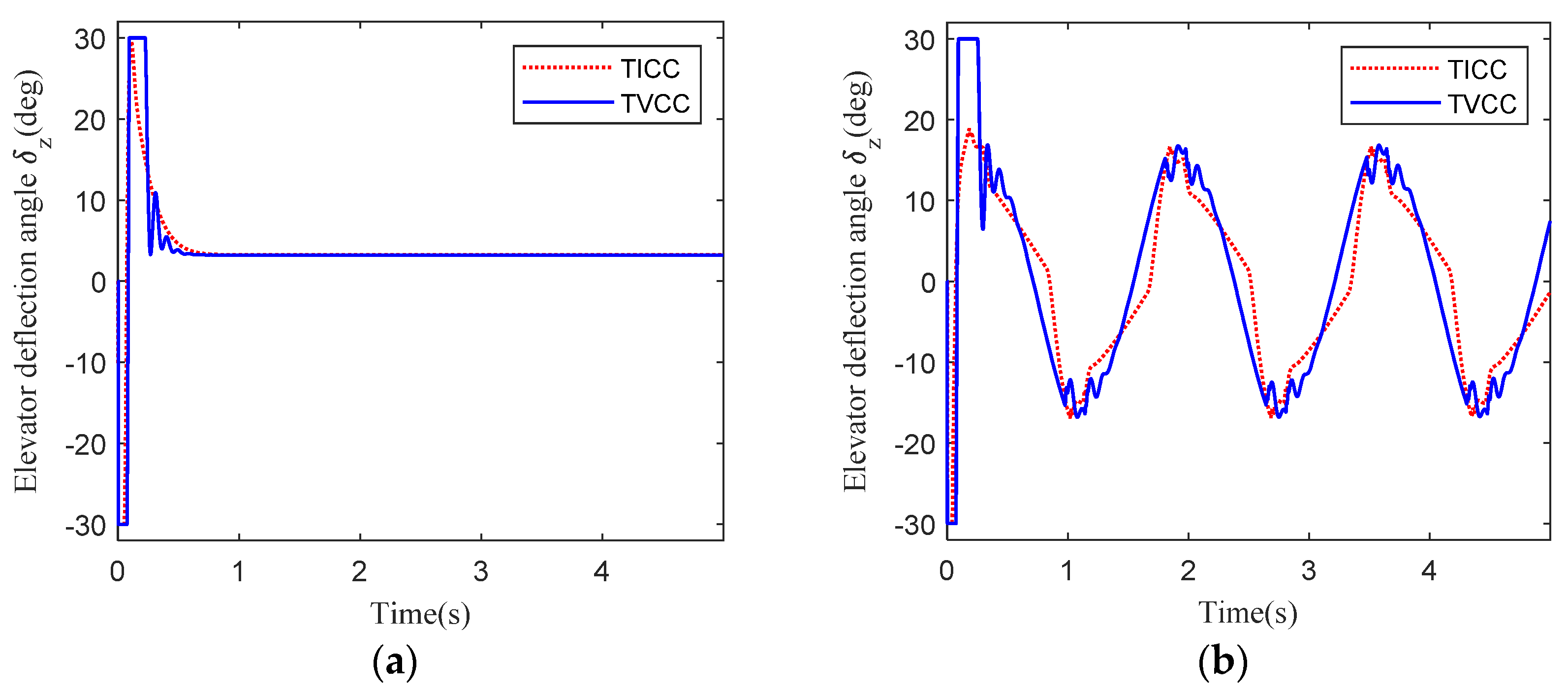
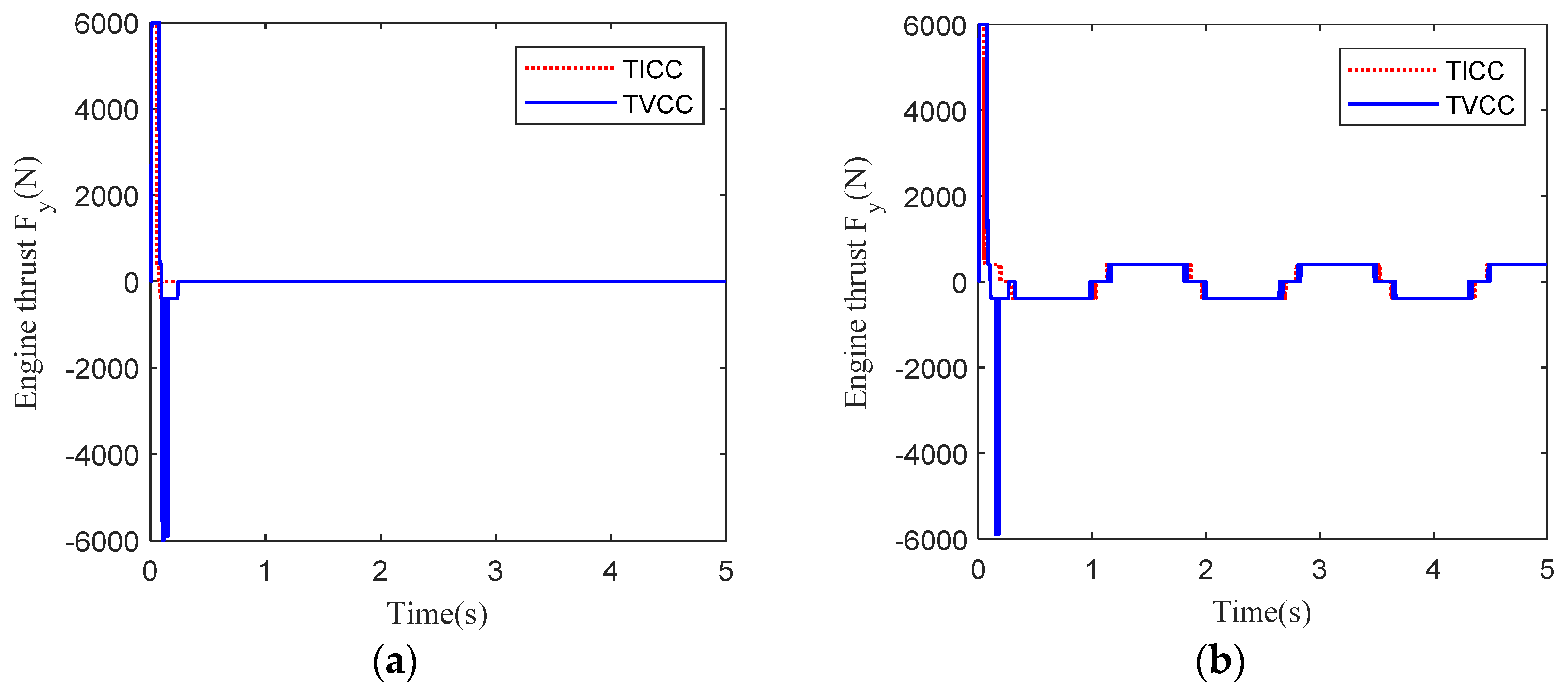
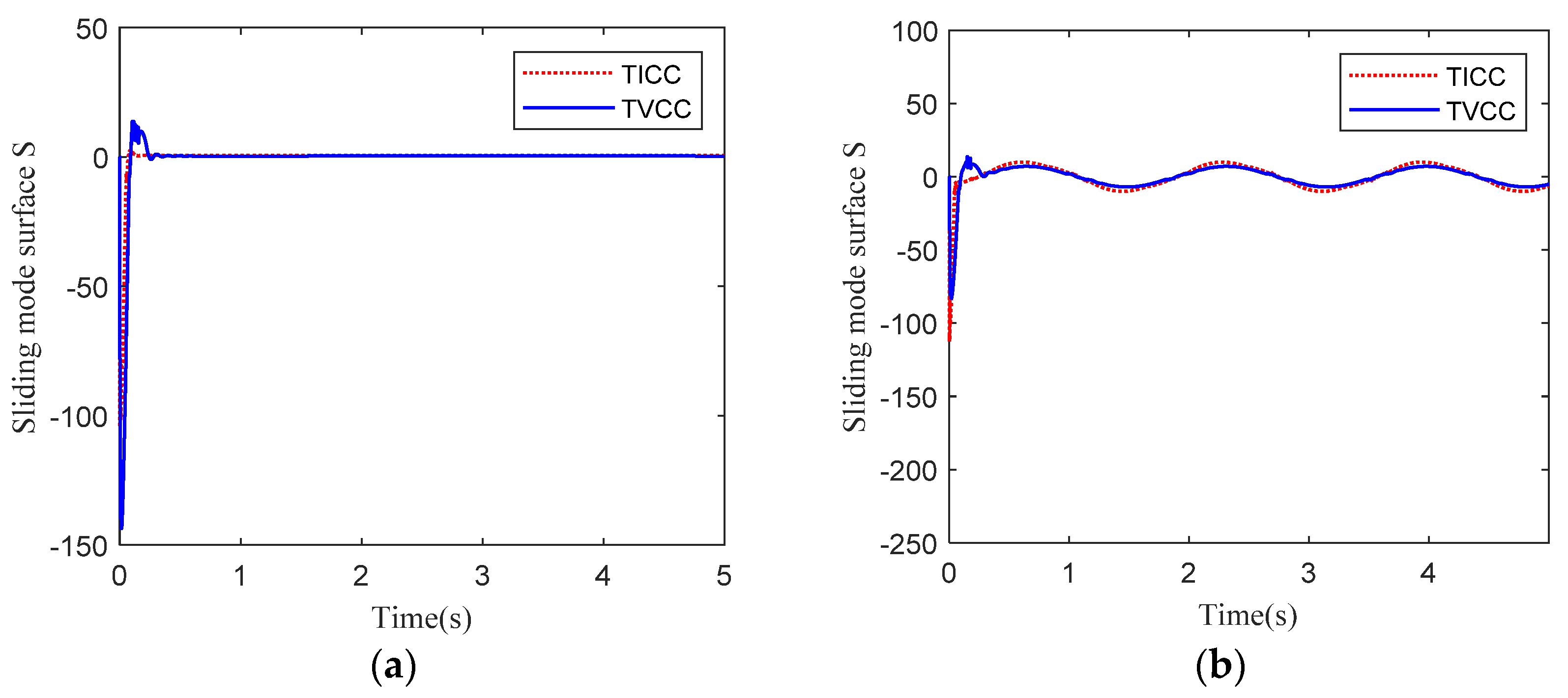
6.2. Simulation Analysis

In order to demonstrate the effectiveness and fast response of the designed time-varying compound control system for the hypersonic vehicle, two simulation cases are given. In the above two cases, the tracking command of normal acceleration is set to be $n_{yc}=10g$.

(1)

Case 1

The simulation results of time-varying single aerodynamic control (TVSAC) and time-varying compound control (TVCC) are shown in Figure 3, Figure 4, Figure 5 and Figure 6. The simulation results of single aerodynamic control refer to the simulation situation when no direct lateral force is added to the system.

As can be seen from Figure 3, Figure 4, Figure 5 and Figure 6, the system with compound control is more stable and responds faster than that with single aerodynamic control when the direct lateral force is added. The tracking response of normal acceleration is shown in Figure 3. The response time of normal acceleration in the compound control system is 0.18 s, the maximum overshoot is less than 3%, and it quickly reaches a stable state. In contrast, the response time of normal acceleration in a single aerodynamic control system is 0.4 s, the maximum overshoot is greater than 3%, and it lasts for a long time before returning to a stable state. Obviously, the response time of the compound control system is faster than that of the single aerodynamic control system.

In Figure 4, the maximum pitch angle rate of the compound control system is 151°/s. As can be seen from the comparison, the pitch rate of the compound control system changes rapidly and becomes stable quickly, while the pitch rate of the single aerodynamic control system takes a longer time to become stable. In Figure 5, in the dynamic process, due to the step change of the normal acceleration instruction and insufficient aerodynamic pressure, the elevator deflection is saturated at the initial stage of the response and remains stable in the steady state process. It can be seen from the comparison that the elevator deflection angle of the single aerodynamic control system has been saturated in the first second; that is, the elevator deflection angle remains at 30°, while the elevator deflection angle of the compound control system quickly returns to a stable state after a short saturation process. In addition, in Figure 6, the variation of the direct lateral force provided by the engine is shown. The side-injection engine only works in the dynamic process, i.e., initial period, and the steady state is always turned off, thus avoiding fuel consumption and disturbance to the system. It can be clearly seen from Figure 6 that in the single aerodynamic control system, the engine is in the shutdown state, and the direct side force is always 0.

According to the above analysis, the time-varying compound control system of the hypersonic vehicle is more stable and has a faster response speed than the single aerodynamic control system.

(2)

Case 2

In order to verify the importance of time-varying compound control design, the simulation results of time-invariant compound control (TICC) and time-varying compound control (TVCC) are compared in Case 2. The effectiveness and fast response of the designed system are demonstrated by tracking the step signal and sinusoidal signal, respectively.

Herein, the time-invariant compound control system means that the controller in the variable parameter system is set to a constant value. Taking a characteristic point in a variable parameter, the time-invariant control law solved by LQR’s Riccati equation in a time-invariant system is designed as $K_1=0.006$, $K_2=-0.17$, $K_3=0.527$, $K_4=0.397$. The simulation results are shown in Figure 7, Figure 8, Figure 9, Figure 10 and Figure 11.

The tracking response of normal acceleration is shown in Figure 7. Among them, the step signal is tracked in Figure 7a, the response time of the TVCC method is 0.2 s, the maximum overshoot is less than 3%, and it quickly reaches a stable state. In contrast, the response time of the TICC method is 0.5 s, and although there is no overshoot, the designed TICC system can better meet the actual requirements for the fast response of the hypersonic vehicle. Similar trends can be seen in Figure 7b. In Figure 8a, the maximum pitch angle rate of the TVCC system is 151°/s, which meets the actual demand. In Figure 8b, it is easy to find that the TICC curve is biased from the sinusoidal signal by comparison. In Figure 9a, in the dynamic process, due to the step change of the normal acceleration instruction and insufficient aerodynamic pressure, the elevator deflection is saturated at the initial stage of the response and remains stable in the steady state process. In the first 0.4 s, which have been saturated, the elevator deflection angle is maintained at 30°, and then quickly stabilized. In Figure 9b, it is obvious that the sinusoidal signal tracked by TVCC has a slight fluctuation but an obvious trend of sinusoidal change, while the sinusoidal signal tracked by TICC has waveform distortion. In Figure 10, the variation of the direct lateral force of the engine is shown. The side-injection engine operates in the dynamic process, and the steady state is turned off, thus avoiding fuel consumption and disturbance to the system. In Figure 11a, the sliding mode surface in the TVCC system rapidly converges to zero and remains there, but the amplitude of the TICC sliding mode surface fluctuates greatly in the initial stage. In Figure 11b, the convergence effect of the TICC sliding mode surface is not as good as that of the TVCC.

In order to highlight that TVCC is more effective than TICC at different flight altitudes, simulation results of the hypersonic vehicle at 25 km are given, as shown in Figure 12, Figure 13, Figure 14, Figure 15 and Figure 16.

The normal acceleration that the hypersonic vehicle needs to track at 25 km is $n_{yc}=15g$. In Figure 12, it is clear that TVCC responds faster than TICC. In Figure 13a, the maximum pitch angle rate of the TVCC system is 205°/s, which meets the actual demand. In Figure 13b, it is easy to find that the TICC curve is biased from the sinusoidal signal by comparison. In Figure 14a, in the first 0.4 s, the elevator deflection angle is maintained at 30°, and then quickly stabilized. In Figure 14b, it is obvious that the sinusoidal signal tracked by TVCC has a slight fluctuation but an obvious trend of sinusoidal change, while the sinusoidal signal tracked by TICC has waveform distortion.

Through the above comparative analysis, the designed time-varying compound control system of the hypersonic vehicle responds faster, is more stable, and has practical significance.

7. Conclusions

A time-varying compound control method is proposed for the hypersonic vehicle controlled by the direct lateral force and the aerodynamic force. The time-varying compound control model is established. The controller for the aerodynamic force control system is designed as a time-varying LQR. To solve the problem that LQR cannot directly obtain the analytical solution of the time-varying system, a novel approach to approximate analytical solutions using Jacobi polynomials is proposed. When the air rudder cannot continuously produce control force and torque, the direct lateral force is added to the system and the sliding mode control method is applied to further solve the control law. The stability of the time-varying compound control system is proven by the Lyapunov–Krasovskii functional. The simulation results show that compared with the single aerodynamic control method and the time-invariant compound control method, the hypersonic vehicle designed with the time-varying compound control method has faster response speed, better stability, and practical significance.

References

1. Tan, Y.; Jing, W.; Gao, C.; An, R. Adaptive improved super-twisting integral sliding mode guidance law against maneuvering target with terminal angle constraint. Aerosp. Sci. Technol. 2022, 129, 107820. [Google Scholar] [CrossRef]
2. Lee, S.; Cho, N.; Kim, Y. Impact-Time-Control Guidance Strategy with a Composite Structure Considering the Seeker’s Field-of-View Constraint. J. Guid. Control. Dyn. 2020, 43, 1566–1574. [Google Scholar] [CrossRef]
3. Zhang, L.; Yang, J.; Duan, T.; Wang, J.; Li, X.; Zhang, K. Numerical and Experimental Investigation on Nosebleed Air Jet Control for Hypersonic Vehicle. Aerospace 2023, 10, 552. [Google Scholar] [CrossRef]
4. Huang, S.; Jiang, J.; Li, O. Adaptive Neural Network-Based Sliding Mode Backstepping Control for Near-Space Morphing Vehicle. Aerospace 2023, 10, 891. [Google Scholar] [CrossRef]
5. Xu, D.; Zhang, J.; Wang, P.; Yan, X.; Dong, H.; Shao, X. Composite Terminal Guidance Law for Supercavitating Torpedoes with Impact Angle Constraints. Math. Probl. Eng. 2022, 1, 65108811. [Google Scholar] [CrossRef]
6. Yu, X.; Luo, S.; Liu, H. Integrated Design of Multi-Constrained Snake Maneuver Surge Guidance Control for Hypersonic Vehicles in the Dive Segment. Aerospace 2023, 10, 765. [Google Scholar] [CrossRef]
7. Zhang, Y.; Shou, Y.; Zhang, P.; Han, W. Sliding mode based fault-tolerant control of hypersonic reentry vehicle using composite learning. Neurocomputing 2022, 484, 142–148. [Google Scholar] [CrossRef]
8. Dong, T.; Zhao, C.; Song, Z. Autopilot Design for a Compound Control Small-Scale Solid Rocket in the Initial Stage of Launch. Int. J. Aerosp. Eng. 2019, 1, 4749109. [Google Scholar] [CrossRef]
9. Sun, W. Research on Thrust Vector/Aerodynamics Compound Control Method Based on Linear Quadratic Regulator Control for Solid Rocket. In Proceeding of the Chinese Automation Congress (CAC), Shanghai, China, 6–8 November 2020; pp. 545–548. [Google Scholar]
10. Liu, Y.; Wang, H.; Wu, T.; Lun, Y.; Fan, J.; Wu, J. Attitude control for hypersonic reentry vehicles: An efficient deep reinforcement learning method. Appl. Soft Comput. 2022, 123, 108865. [Google Scholar] [CrossRef]
11. Zhang, B.; Liang, Y.; Rao, S.; Kuang, Y.; Zhu, W. RBFNN-Based Anti-Input Saturation Control for Hypersonic Vehicles. Aerospace 2024, 11, 108. [Google Scholar] [CrossRef]
12. Mechali, O.; Xu, L.; Huang, Y.; Shi, M.; Xie, X. Observer-based fixed-time continuous nonsingular terminal sliding mode control of quadrotor aircraft under uncertainties and disturbances for robust trajectory tracking: Theory and experiment. Control. Eng. Pract. 2021, 111, 104806. [Google Scholar] [CrossRef]
13. Yun, Y.; Tang, S.; Guo, J.; Shang, W. Robust controller design for compound control missile with fixed bounded convergence time. J. Syst. Eng. Electron. 2018, 29, 116–133. [Google Scholar] [CrossRef]
14. Sun, J.; Liu, C. Auxiliary-system-based composite adaptive optimal backstepping control for uncertain nonlinear guidance systems with input constraints. ISA Trans. 2020, 107, 294–306. [Google Scholar] [CrossRef] [PubMed]
15. Lv, X.; Zhang, G.; Bai, Z.; Zhou, X.; Shi, Z.; Zhu, M. Adaptive Neural Network Global Fractional Order Fast Terminal Sliding Mode Model-Free Intelligent PID Control for Hypersonic Vehicle’s Ground Thermal Environment. Aerospace 2023, 10, 777. [Google Scholar] [CrossRef]
16. Jiang, W.; Wu, K.; Wang, Z.; Wang, Y. Gain-scheduled control for morphing aircraft via switching polytopic linear parameter-varying systems. Aerosp. Sci. Technol. 2020, 107, 106242. [Google Scholar] [CrossRef]
17. Yue, T.; Wang, L.; Ai, J. Gain self-scheduled H∞ control for morphing aircraft in the wing transition process based on an LPV model. Chin. J. Aeronaut. 2013, 26, 909–917. [Google Scholar] [CrossRef]
18. He, Z.; Yin, M.; Lu, Y.-p. Tensor product model-based control of morphing aircraft in transition process. Proc. Inst. Mech. Eng. Part G J. Aerosp. Eng. 2015, 230, 378–391. [Google Scholar] [CrossRef]
19. Galván-Guerra, R.; Fridman, L. Robustification of time varying linear quadratic optimal control based on output integral sliding modes. IET Control. Theory Appl. 2015, 9, 563–572. [Google Scholar] [CrossRef]
20. Lan, J.; Zhao, D. Finding the LQR Weights to Ensure the Associated Riccati Equations Admit a Common Solution. IEEE Trans. Autom. Control 2023, 68, 6393–6400. [Google Scholar] [CrossRef]
21. Abdallah, N.B.; Chouchene, F. New recurrence relations for Wilson polynomials via a system of Jacobi type orthogonal functions. J. Math. Anal. Appl. 2021, 498, 124978. [Google Scholar] [CrossRef]
22. Zhang, H.-Y.; Luo, J.-Z.; Zhou, Y. Explicit Symplectic-Precise Iteration Algorithms for Linear Quadratic Regulator and Matrix Differential Riccati Equation. IEEE Access 2021, 9, 105424–105438. [Google Scholar] [CrossRef]
23. Bhattacharya, R. Robust LQR design for systems with probabilistic uncertainty. Int. J. Robust Nonlinear Control 2019, 29, 3217–3237. [Google Scholar] [CrossRef]
24. Aipanov, S.A.; Murzabekov, Z.N. Analytical solution of a linear quadratic optimal control problem with control value constraints. J. Comput. Syst. Sci. Int. 2014, 53, 84–91. [Google Scholar] [CrossRef]
25. Boukadida, W.; Benamor, A.; Messaoud, H. Multi-Objective Design of Optimal Sliding Mode Control for Trajectory Tracking of SCARA Robot Based on Genetic Algorithm. J. Dyn. Syst. Meas. Control 2019, 141, 031015. [Google Scholar] [CrossRef]
26. Hu, S.; Wang, J.; Wang, Y.; Tian, S. Stability Limits for the Velocity Orientation Autopilot of Rolling Missiles. IEEE Access 2021, 9, 110940–110951. [Google Scholar] [CrossRef]
27. Lee, S.; Cho, N.; Shin, H.-S. Analysis of Guidance Laws With Nonmonotonic Line-of-Sight Rate Convergence. IEEE Trans. Aerosp. Electron. Systems 2022, 58, 1029–1041. [Google Scholar] [CrossRef]
28. Guo, J.; Li, Y.; Zhou, J. Qualitative indicator-based guidance scheme for bank-to-turn missiles against couplings and maneuvering targets. Aerosp. Sci. Technol. 2020, 106, 106196. [Google Scholar] [CrossRef]
29. Zhou, Z.; Liu, Z.; Pan, Y.; Yi, J. Controller design and stability analysis for spinning missiles via tensor product. Aerosp. Sci. Technol. 2022, 130, 107877. [Google Scholar] [CrossRef]
30. Qiao, H.; Meng, H.; Ke, W.; Gao, Q.; Wang, S. Adaptive control of missile attitude based on BP–ADRC. Aircr. Eng. Aerosp. Technol. 2020, 92, 1475–1481. [Google Scholar] [CrossRef]
31. Li, W.; Wen, Q.; Yang, Y. Stability analysis of spinning missiles induced by seeker disturbance rejection rate parasitical loop. Aerosp. Sci. Technol. 2019, 90, 194–208. [Google Scholar] [CrossRef]
32. Zhou, T.; Cai, G.; Zhou, B. Further results on the construction of strict Lyapunov–Krasovskii functionals for time-varying time-delay systems. J. Frankl. Inst. 2020, 357, 8118–8136. [Google Scholar] [CrossRef]
33. Zhou, B. Construction of strict Lyapunov–Krasovskii functionals for time-varying time-delay systems. Automatica 2019, 107, 382–397. [Google Scholar] [CrossRef]
34. Lin, S.-D.; Chao, Y.-S.; Srivastava, H.M. Some families of hypergeometric polynomials and associated integral representations. J. Math. Anal. Appl. 2004, 294, 399–411. [Google Scholar] [CrossRef]
35. Ma, C.; Malyarenko, A. Time-Varying Isotropic Vector Random Fields on Compact Two-Point Homogeneous Spaces. J. Theor. Probab. 2018, 33, 319–339. [Google Scholar] [CrossRef]
36. Aksikas, I.; Forbes, J.F.; Belhamadia, Y. Optimal control design for time-varying catalytic reactors: A Riccati equation-based approach. Int. J. Control. 2009, 82, 1219–1228. [Google Scholar] [CrossRef]
37. Athans, M.; Falb, P.L. Optimal Control. In An Introduction to the Theory and Its Applications; McGraw-Hill: New York, NY, USA, 2007. [Google Scholar]
38. Kwakernaak, H.; Sivan, R. Linear Optimal Control Systems; John Wiley, Ed.; Wiley-interscience: New York, NY, USA, 1972. [Google Scholar]
39. Kalenova, V.I.; Morozov, V.M. A new class of reducible linear time-varying systems and its relation to the optimal control problem. J. Appl. Math. Mech. 2016, 80, 105–112. [Google Scholar] [CrossRef]
Figure 1. The solution process of LQR time-varying control law.
Aerospace 11 00567 g001
Figure 2. The variation range of aerodynamic parameter a 4 ( t ) .
Aerospace 11 00567 g002
Figure 3. The response of normal acceleration in case 1.
Aerospace 11 00567 g003
Figure 4. The response of pitch rate in case 1.
Aerospace 11 00567 g004
Figure 5. The response of elevator deflection in case 1.
Aerospace 11 00567 g005
Figure 6. Variations of lateral thrust in case 1.
Aerospace 11 00567 g006
Figure 7. Simulation comparison of the normal acceleration response curves at 30 km in case 2. (a) Tracking step signal; (b) Tracking sinusoidal signal.
Aerospace 11 00567 g007
Figure 8. Simulation comparison of the pitch rate response curves at 30 km in case 2. (a) Tracking step signal; (b) Tracking sinusoidal signal.
Aerospace 11 00567 g008
Figure 9. Simulation comparison of the elevator deflection angle response curves at 30 km in case 2. (a) Tracking step signal; (b) Tracking sinusoidal signal.
Aerospace 11 00567 g009
Figure 10. Simulation comparison of the engine thrust variation curves at 30 km in case 2. (a) Tracking step signal; (b) Tracking sinusoidal signal.
Aerospace 11 00567 g010
Figure 11. Simulation comparison of the sliding mode function variation curves at 30 km in case 2. (a) Tracking step signal; (b) Tracking sinusoidal signal.
Aerospace 11 00567 g011
Figure 12. Simulation comparison of the normal acceleration response curves at 25 km in case 2. (a) Tracking step signal; (b) Tracking sinusoidal signal.
Aerospace 11 00567 g012
Figure 13. Simulation comparison of the pitch rate response curves at 25 km in case 2. (a) Tracking step signal; (b) Tracking sinusoidal signal.
Aerospace 11 00567 g013
Figure 14. Simulation comparison of the elevator deflection angle response curves at 25 km in case 2. (a) Tracking step signal; (b) Tracking sinusoidal signal.
Aerospace 11 00567 g014
Figure 15. Simulation comparison of the engine thrust variation curves at 25 km in case 2. (a) Tracking step signal; (b) Tracking sinusoidal signal.
Aerospace 11 00567 g015
Figure 16. Simulation comparison of the sliding mode function variation curves at 25 km in case 2. (a) Tracking step signal; (b) Tracking sinusoidal signal.
Aerospace 11 00567 g016