Article

On the Generalization Capability of a Data-Driven Turbulence Model by Field Inversion and Machine Learning

Center for Computer Applications in AeroSpace Science and Engineering, Institute of Aerodynamics and Flow Technology, German Aerospace Center (DLR), Bunsenstr. 10, 37073 Göttingen, Germany
*
Author to whom correspondence should be addressed.
Aerospace 2024, 11(7), 592; https://doi.org/10.3390/aerospace11070592
Submission received: 30 May 2024 / Revised: 11 July 2024 / Accepted: 12 July 2024 / Published: 20 July 2024
(This article belongs to the Special Issue Data-Driven Aerodynamic Modeling)

Abstract

:
This paper discusses the generalizability of a data-augmented turbulence model with a focus on the field inversion and machine learning approach. It is highlighted that the augmented model based on two-dimensional (2D) separated airfoil flows gives poor predictive capability for a different class of separated flows (NASA wall-mounted hump) compared to the baseline model due to extrapolation. We demonstrate a sensor-based approach to localize the data-driven model correction to tackle this generalizability issue. Furthermore, the applicability of the augmented model to a more complex aeronautical three-dimensional case, the NASA Common Research Model configuration, is studied. Observations on the pressure coefficient predictions and the model correction field suggest that the present 2D-based augmentation is to some extent applicable to a three-dimensional aircraft flow.

1. Introduction

While scale-resolving simulations for turbulent flows, such as large-eddy simulations (LES) or direct numerical simulations (DNS), are becoming realizable at low to modest Reynolds numbers due to the continuous increase in computational resources, they are still too expensive to be used in most of today’s industrial aerodynamic design processes. Hence, Reynolds-averaged Navier–Stokes (RANS) simulations have been a standard tool, which deal with the statistically averaged mean flow equations and model all turbulent scales. While RANS computations provide fast and reliable prediction for canonical flows, there are still challenges to accurately simulate complex flows, including adverse pressure gradient flows and vortical flows. Despite the importance of the modeling of such flow phenomena and much progress achieved in this field, the developments with classical approaches seem to have stagnated in the past decades [1]. This has motivated the turbulence modeling community to utilize the fast-growing machine learning techniques as a new tool to give new impetus to RANS model improvement.
Some of the pioneering works in data-driven turbulence modeling include the Gene Expression Programming (GEP) of Weatheritt and Sandberg [2], the Sparse Regression of Turbulent stress Anisotropy (SpaRTA) symbolic-regression approach of Schmelzer et al. [3], the Tensor Basis Neural Network (TBNN) of Ling et al. [4], and the Field Inversion and Machine Learning (FIML) of Singh and Duraisamy [5]. The first two are often classified as “open-box” approaches that provide explicit mathematical expressions that can be easily incorporated into existing CFD solvers and can allow the modelers to verify the physical plausibility of the derived model. The latter two approaches are usually referred to as “black-box” or “gray-box” techniques due to their use of artificial neural networks (ANNs) or random forests, which offer flexible approximations of the complex mapping between flow features and targeted model correction terms. Although all those frameworks have shown their potential to offer improved predictive capability, it has been revealed that they share a common issue: the data-driven models perform well only for flow cases that are very similar to the training cases. Moreover, most of the works in the literature are restricted to the investigation of relatively simple two-dimensional flow configurations. Three-dimensional, industry-relevant complex flows are typically involved with multiple characteristic flow phenomena at different locations. In such a scenario, an ideal data-driven model should be sensible to each physical phenomenon and be modified from the original form wherever necessary while preserving the baseline model’s accuracy at worse. To this date, such a general model has not been found by data-driven methods to the authors’ best knowledge. It should be noted that recent efforts towards improving the generalizability of the data-driven models are found in, e.g., [6,7].
In the present paper, our aim is not to present a new generalizable data-driven model, but is to analyze the generalizability of one data-driven model obtained in [8] in both 2D- and 3D-flows including flow scenarios that are different from training cases. In addition, we present a sensor-based approach to localize the model augmentation and demonstrate it in 2D examples.
The structure of the paper is as follows: In Section 2, we briefly summarize the FIML approach and the training strategy of the model we consider in this paper. Section 3 addresses the evaluations for the 2D-flow cases, and in Section 4, we discuss the applicability of the 2D-based model to an industry-relevant 3D aircraft flow configuration.

2. Methodology

In the present work, we focus on one data-driven turbulence model presented in [8]. Therein, the baseline model is the negative Spalart–Allmaras (SA-neg) turbulence model [9], which was enhanced in [8] by training for several 2D airfoil flows using experimental data via the field inversion and machine learning framework.
While the reader is referred to the original publication for a comprehensive description, the fundamentals of the FIML approach and the brief descriptions of the chosen machine learning model are given in Section 2.1 and Section 2.2, respectively. The numerical method to solve the compressible RANS equations with the augmented SA-neg model is given in Section 2.3. Finally, in Section 2.4, we present an approach to localize the application of the model augmentation in attached turbulent boundary layers in an adverse pressure gradient, which will be demonstrated for 2D-flows in Section 3.

2.1. Field Inversion and Machine Learning

The field inversion and machine learning method, originally proposed in [5], is an approach that allows to augment an existing turbulence model by making use of high-fidelity data and machine learning techniques. The fundamental idea is to introduce a model correction term into a baseline turbulence model and to train a machine learning model (e.g., neural network) that predicts the correction term based on the local flow states. The baseline model we consider is the negative Spalart–Allmaras turbulence model (SA-neg) [9], and the correction term β is introduced as a multiplier of the production term, which reads
D ν ˜ D t = β P D + 1 σ · ( ( ν + ν ˜ ) ν ˜ ) + c b 2 ( ν ˜ ) 2 ,
where ν ˜ denotes the SA variable, P is the production term, and D is the destruction term. Note that ν is the kinematic viscosity, and c v 1 , c b 2 , and σ are model-specific constants (see the original publications [9] for the details).
Given high-fidelity reference data, such as experimental data for a certain flow case, one can formulate an inverse problem for finding an optimal field of β , which minimizes the discrepancy between the RANS solution and the reference solution. More formally, a cost function such as
I = 1 2 V t o t i N V i ( q i , r e f q i , R A N S ( β ) ) 2
is minimized while all the governing equations are satisfied. Here, q i , r e f and q i , R A N S are, respectively, the reference solution and its RANS prediction of the quantity of interest at the i-th grid cell. The N denotes the total number of grid cells, V i is the cell volume at the i-th cell, and V t o t is the total cell volume. The optimized β field is obtained by solving this inverse problem; however, those values are not directly applicable to a new simulation with different flow conditions or geometry. To this end, another key element of the FIML is to find a functional mapping between the correction term β and the flow state ( U , ν ˜ ), such that one can predict the field of β for an unseen flow case. Typically, a set of non-dimensional quantities derived from the flow state ( U , ν ˜ ), often called “flow features” η , is selected, and a machine learning model, such as a neural network, that maps the feature space η to β is trained.
The above-mentioned inversion process and the training of the machine learning model can be performed with separated two-steps or with an integrated single step. The former is often referred to as the classic FIML, which corresponds to the approach presented in [5]. On the other hand, the d i r e c t FIML is the latter approach proposed in [10] and also used for the model we use in the present work. While in the classic FIML, the design variable of the inverse optimization problem is the field of β , in the direct FIML, the design variable is the machine learning model parameter w , and the field of β is predicted by the embedded ML model during the entire process. Thus, the cost function can be rewritten as
I = 1 2 V t o t i N V i ( q i , r e f q i , R A N S ( β ( η , w ) ) ) 2 .
The workflow of the FIML framework is depicted in Figure 1. Note that due to the high-dimensional nature of the inverse problem posed here, a gradient-based optimization method is preferred and thus the adjoint method is utilized.

2.2. A Closed-Form Correction with Radial Basis Function

While the FIML approach is often used with black-box machine learning algorithms, such as neural networks, Jäckel (2023) [8] presented a closed-form model correction using a Gaussian radial basis function (RBF):
β η i = 1 β ^ e i η i η 0 , i 2 a i
where η i are the input flow features and three features were used in his work,
η 1 = log 10 P D , η 2 = log 10 ν ˜ ν , η 3 = log 10 ν t | S | u τ 2
where ν t denotes the turbulent viscosity, S the strain rate, and u τ the friction velocity mapped from the wall surfaces to all nearest field points. Due to the closed-form expression, it is better interpretable than the one with neural networks. The model was optimized through the multi-case direct FIML training (see the list of training cases in Table 1), and the resulting model parameter values are summarized below
β ^ = 0.7059 η 0 , 0 = 1.372 , η 0 , 1 = 1.959 , η 0 , 2 = 0.7328 a 0 = 1.607 , a 1 = 1.993 , a 2 = 1.437 .
Throughout this paper, we use this specific RBF model to augment the original SA-neg model.

2.3. Numerical Set-Up

The DLR TAU-code [13] is used as the CFD solver, which is a compressible, cell-vertex-type finite-volume solver with dual-control volumes. A discrete adjoint solver is also available in the TAU-code [14] and is used in the field inversion process. An implicit backward Euler scheme with the lower-upper symmetric Gauss–Seidel (LU-SGS) scheme is used for obtaining steady-state flow solutions.
For the FIML framework, the TAU code is coupled with the DLR’s SMARTy (Surrogate Modeling for AeRo data Toolbox Python Package) toolbox [15], which is a modular Python package (API) providing various data-driven techniques for aerodynamic simulations. It offers a Python-level interface to operate TAU and wrappers around popular deep-learning frameworks, such as PyTorch [16], which enables a flexible way of integrating the existing CFD solver TAU and fast-growing external machine learning libraries.

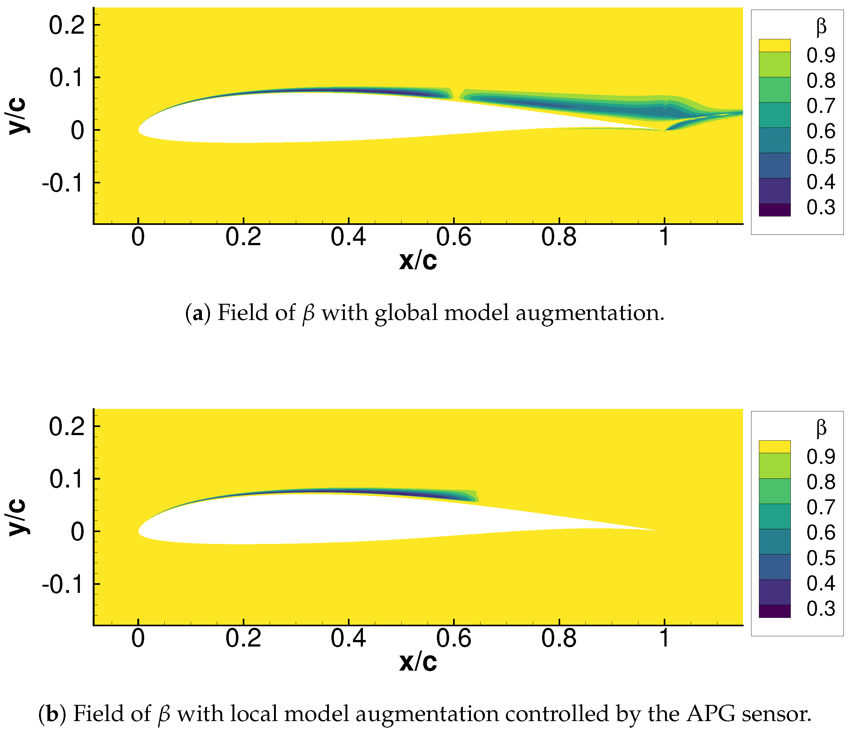
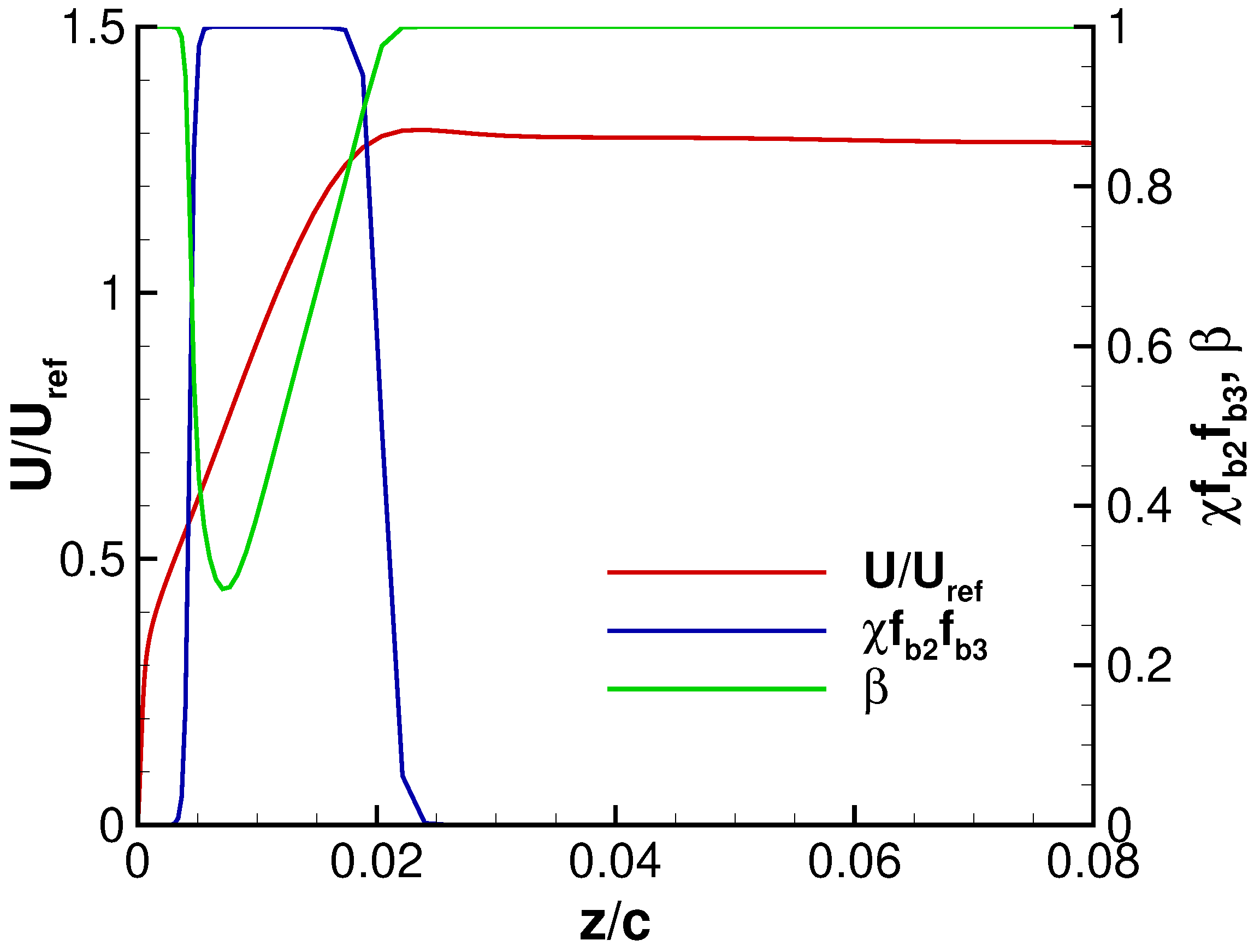
2.4. Localized Model Correction with Sensor Functions for Adverse Pressure Gradient Flows

In Section 3, we demonstrate an approach to locally apply the data-driven model corrections by using sensor functions designed for the attached turbulent boundary layers in an adverse pressure gradient. The rationale behind this idea is that a data-driven model is only applicable to flows that are very similar to its training cases, and, therefore, the model augmentation should be deactivated where the local flow state is far from the training scenarios. The necessity of different sets of model coefficients depending on the local type of flow is also suggested in [17] based on the analysis of equilibrium turbulent flows. The methodology presented here and the results shown in Section 3 are partly published as a conference proceedings paper [18]. The conference paper includes an additional study with a machine learning-based sensor to localize the model augmentation.
In the present work, we reformulated the production term β P of the original FIML implementation such that ( 1 f ) P + f β P , where f is a blending factor ranging from 0 to 1. Here, with f = 1 everywhere, it falls back to the original FIML formulation, i.e., “global” model correction. This reformulation is inspired by the work of Ling and Kurzawski (2017) [19], where they blended a linear eddy-viscosity model and a quadratic eddy-viscosity model in a similar manner. The choice of suitable sensors is not trivial, but the present work utilizes a set of sensor functions proposed in [20], which is used to modify the ω -equation of the SSG/LRR- ω model for adverse pressure gradient (APG) flows. The sensor is composed of three functions χ f b 2 f b 3 and is designed to detect the so-called half-power law region emerging above the classical log-law region in APG turbulent boundary layer flows. However, the data-driven model used here is not specifically targeted to the half-power law region, and thus, we slightly adjusted them to detect the region up to the edge of the boundary layer in this work. The values of χ f b 2 f b 3 are designed to range between 0 and 1, and thus the modified production term reads ( 1 χ f b 2 f b 3 ) P + χ f b 2 f b 3 β P .
The three sensor functions are briefly described in the following: The first function χ = χ Δ p s + , u τ / U e is an activation function that determines if the flow is at APG and also if the flow is attached based on the boundary layer edge velocity U e , and the non-dimensional pressure gradient parameter Δ p s + = ( ν / ρ u τ 3 ) d P / d s . Therein, d P / d s denotes the streamwise pressure gradient and u τ the friction velocity. The χ becomes unity where Δ p s + > Δ p 0 + and u τ / U e > 0 . The threshold value Δ p 0 + is set to 8 × 10 6 . The sign of u τ / U e is calculated by taking the inner product of the velocity vector at the first node off the wall and the edge velocity vector.
The second function f b 2 acts as a blending function that shields the classical log-law region.
f b 2 = 0.5 ( tanh ( ζ ) + 1 ) , ζ = y + y incpt + c b 2 c s 2 1 y sqrt , min + c s 2 y log , max +
with c b 2 = 0.5 , c s 2 = 1.04 , and y incpt + = 0.5 ( y sqrt , min + + y log , max + ) . The y log , max + defines the outer edge of the log-law region and the y sqrt , min + is the location above which the half-power law region emerges. These are determined by the empirical correlations based on the friction Reynolds number R e τ = δ u τ / ν and Δ p s + , which read
y log , max + = 1.68 Re τ 1 / 2 Δ p s + 1 / 5 ,
y sqrt , min + = 4.05 Re τ 1 / 2 Δ p s + 0.13 ,
where δ = δ 99 / 0.94 is applied. The f b 2 becomes zero below the outer part of the log-law region and rapidly increases towards one in the border with the half-power law region.
The third function f b 3 is another blending function, which determines the upper limit of the modification:
f b 3 = 1 0.5 ( tanh ( ξ ) + 1 ) ,
ξ = η η m 3 c b 3 η u 3 η l 3 , η = y δ
with c b 3 = 0.525 and η m 3 = 0.5 η l 3 + η u 3 . The value of f b 3 becomes approximately unity where y / δ < η l 3 and f b 3 0 for y / δ > η u 3 . Here, η l 3 = 0.95 , η u 3 = 1.05 are used in the present work, meaning f b 3 remains unity up to the edge of the boundary layer. Note that η l 3 = 0.2 , η u 3 = 0.27 are used in the original work [20].

3. Two-Dimensional Flow Cases

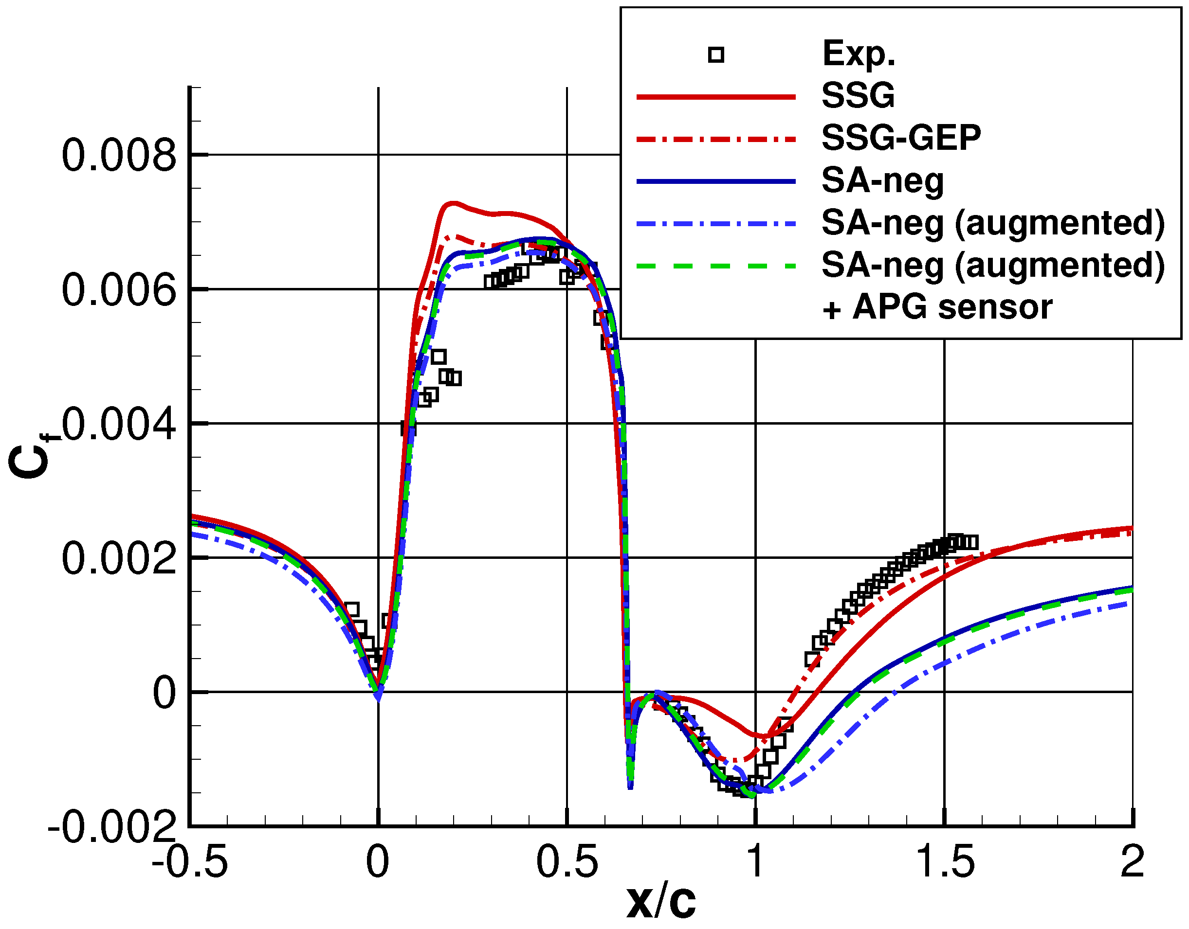
3.1. NASA Wall-Mounted Hump
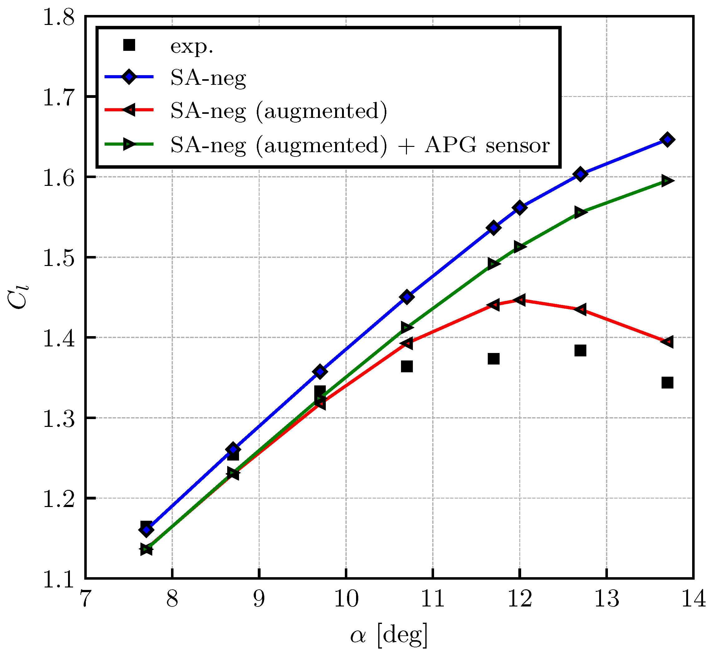
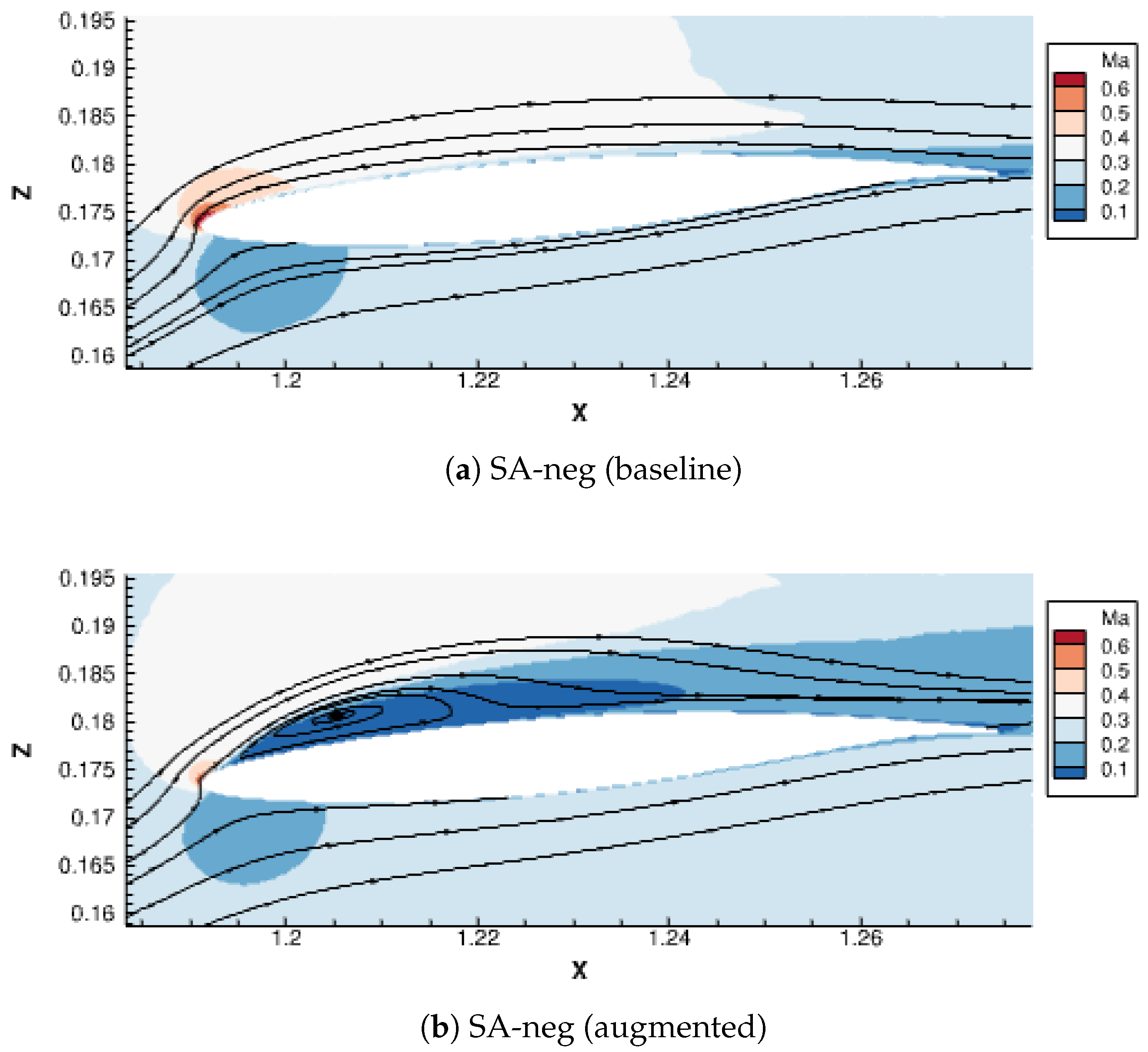
The augmented SA-neg model trained for multiple airfoil flows with separation has been tested on the 2D NASA wall-mounted hump (no plenum) case [21]. The flow conditions are Mach number M a = 0.1 and the Reynolds number based on the hump chord R e c = 936,000. It is a representative test case of flow separation and reattachment on a smooth surface with pressure gradients. For this case, traditional RANS turbulence models are known to produce a delayed reattachment due to the under-prediction of the Reynolds stresses. While this case exhibits flow separation due to an adverse pressure gradient as in airfoil flow cases, it should be seen as a slightly different class of flows in terms of turbulence modeling. In airfoil flows at high incidence angles, traditional RANS models tend to underpredict trailing-edge separation and the resulting overprediction of the lift coefficient is a primary challenge. Here, the reattachment point in a steady simulation is more or less fixed at the trailing edge. On the other hand, for the class of NASA hump flows, the primary attention is typically more on the reattachment prediction rather than the separation onset, which is mostly fixed by the strong pressure rise due to a sudden change in geometry.
Figure 2 shows comparisons of the skin friction coefficient. As can be seen, the augmented model exhibits the flow reattachment further downstream than the baseline SA-neg model, which is already far from the experimental data. This is an example where a data-driven model gives a worse prediction than its original model due to undesired model corrections. Typically, this occurs due to extrapolation of the machine learning model, meaning that the model makes prediction based on data that lie outside the scope of the training data. In this particular case, the machine learning model predicts the correction term β based on the local flow features ( η 1 3 ) at each grid point. If the values of those flow features are far from the training data’s counterpart, the prediction of β at that grid point by the machine learning model would have high uncertainty. This uncertainty, i.e., the extent of extrapolation, can be quantified by using some distance metric, such as the Mahalanobis distance, which will be detailed later. Furthermore, even if there exist close training data (i.e., η 1 3 η 1 3 t r a i n ), a completely different correction term might be required. This could happen when the selected flow features are insufficient to discern different underlining flow physics and/or when the coverage of the training data is insufficient. In Figure 2, the results of another data-driven model by gene-expression programming (GEP) trained in [22] are also shown together with its baseline Speziale–Sarkar–Gatski (SSG) model [23]. The SSG-GEP model here was trained using large-eddy simulation (LES) data for the curved backward-facing step by Bentaleb et al. (2012) [24], whose nature is the same as the NASA hump case. As anticipated, it shows a better reattachment prediction as extrapolation should not happen as much as the augmented SA-neg model and interpolation is dominant. Despite the difference in the underlining machine learning techniques, it illustrates that the prediction of the present NASA hump test case can be improved by a data-driven model with small extrapolation extent.
The aforementioned Mahalanobis distance metric, which can quantify the extrapolation extent, has been tested to obtain further insight, following [25]. The Mahalanobis distance is a distance metric similar to the Euclidean distance; however, it only requires to store the mean and covariance matrices of the training data to assess the extrapolation extent for a new case. The Euclidean distance between an evaluation point and one of the training data samples in the feature space reads
D e = i = 1 3 ( η i η i t r a i n ) 2 ,
where η i are the flow features at a grid point of evaluation and η i t r a i n are those of the training sample. By using this metric and the nearest neighbor search technique, the extrapolation extent, i.e., how far the current data point is off from the training dataset, could be quantified. However, this would require to store the entire training data samples. In contrast, the Mahalanobis distance has a low memory requirement and provides similar quality to the nearest neighbor Euclidean distance metric, as reported in [25]. The Mahalanobis distance between an evaluation point and the distribution of the training data in feature space is calculated as
D m = ( η μ ) T V 1 ( η μ ) ,
where μ and V 1 are the mean and inverse covariance matrix of the training data, respectively. Note that the matrix notation is used for the flow features η .
For the augmented SA-neg model, the Mahalanobis distance is evaluated on the NASA hump case (Figure 3). It can be observed that the extrapolation extent is higher (i.e., high value of the Mahalanobis distance) in the region of the separated shear layer.
The local model correction with the APG TBL sensor that was described in the previous section was also tested. As shown in Figure 2, the prediction of the augmented model with the sensor functions is almost the same as that of the baseline model. A comparison of the field of β is illustrated in Figure 4. In global model augmentation, model correction is active in a large part of the boundary layer (except the first half of the hump 0 < x / c < 0.6 ), as well as inside a separation bubble. This includes a zero and favorable pressure gradient region in the upstream ( x / c < 1 ) and downstream of the hump ( x / c > 1.5 ) (see Figure 5 for the pressure coefficient distribution). Model corrections in those region have been suppressed by the introduction of the sensor, mainly the χ activation function that detects an adverse pressure gradient region. Most of the model correction inside the separation bubble is also deactivated, which is again presumably due to the χ activation function that additionally excludes a separated boundary layer region.
As demonstrated here, the APG TBL sensor serves as a limiter or an additional “safety-net” to preserve the predictive capability of the baseline model for untrained, non-airfoil flows. The effect of introducing the sensor for trained, airfoil flow cases will be discussed in the following section.

3.2. HGR-01 Airfoil

The global and localized model corrections with the sensor are also compared for the HGR-01 airfoil, whose 13.7 deg case was used as one of the training cases. The HGR-01 airfoil was designed at the Technische Universität Braunschweig to study the mixed leading-edge trailing-edge stall behavior [12]. The flow conditions are M a = 0.07 and R e c = 0.65 × 10 6 , and the transition is fixed using experimentally measured transition locations. It is fixed at x / c = 0.002 on the suction side and at x / c = 0.95 on the pressure side.
Figure 6 shows the comparisons of the lift coefficient curve. Firstly, it should be highlighted that the global model augmentation, SA-neg (augmented), gives a consistent improvement in the lift prediction, while only one of the incidence angles was seen during the training phase. Although not shown, the same holds for the S809 airfoil cases at various angles of attack.
On the other hand, the local model augmentation, SA-neg (augmented) + APG sensor, loses more prediction accuracy as the angle of attack increases. This can be explained as follows: As shown in Figure 7a, there are two distinct regions where model correction is active. The first region around 0 < x < 0.6 is in an attached boundary layer, and the second one around x > 0.6 corresponds to the region downstream of the separation point. At low angles of attack, model corrections in the latter are not dominant since the separation occurs close to the trailing edge. However, at high angles of attack, their contribution to the entire lift change becomes significant due to the earlier separation. The APG sensor deactivates the model correction in this post-separation region (Figure 7b), and thus the accuracy loss becomes larger at higher incidence angles.
In addition, Figure 8 shows the profile of the sensor value χ f b 2 f b 3 and β at the location of x / c = 0.5 for the local model augmentation. The velocity profile normalized by the reference velocity is also given. An increase in the sensor value from 0 to 1 at z / c 0.005 is controlled by f b 2 and a decrease at z / c 0.02 is controlled by the values of the f b 3 function. Note that χ , which is an activation function to determine an adverse pressure gradient and flow separation, does not play a role on this wall normal profile. It can be observed that the value of χ f b 2 f b 3 drops to zero, as expected, at around the location where the velocity takes its maximum value. Also, the value of β is shielded in the near wall region ( z / c < 0.005 ) due to the f b 2 function.
The accuracy loss by the local model augmentation is inevitable for this case, as the global model augmentation should be seen as a locally optimal solution. The extent of the accuracy loss is solely due to the a posteriori usage of the APG sensor function, which only detects an attached boundary layer. Although still far from ideal, the data-augmentation with this type of physics-based sensor could offer a compromised model, which provides some improvement for target flow phenomena while not losing the predictive capability of the baseline model at worse.

4. Application to Three-Dimensional Flows

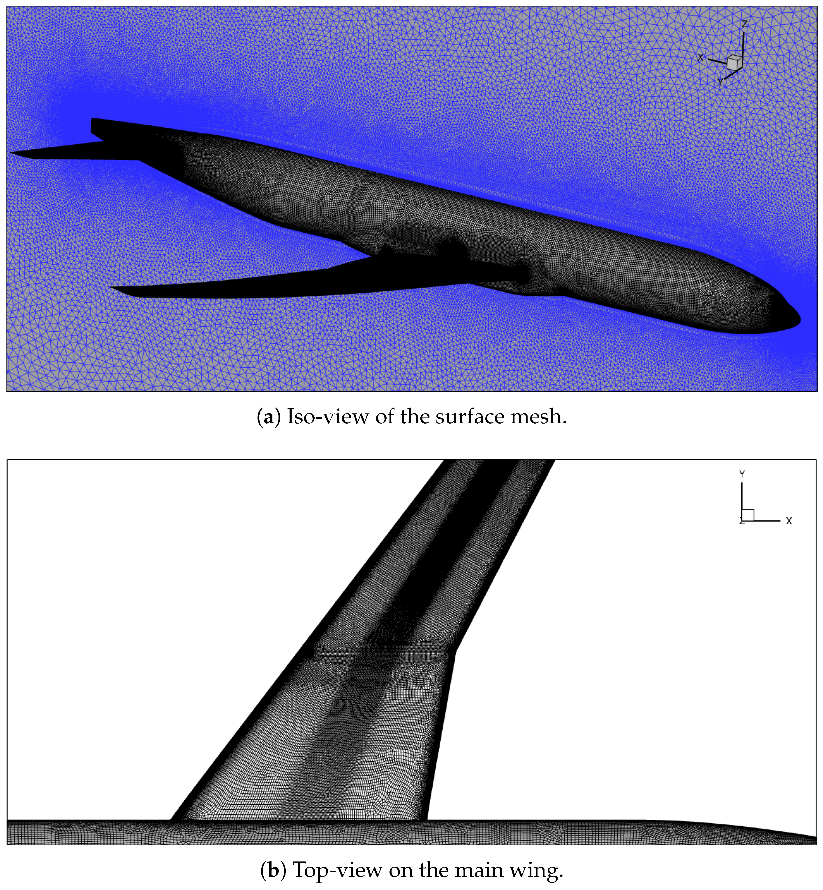
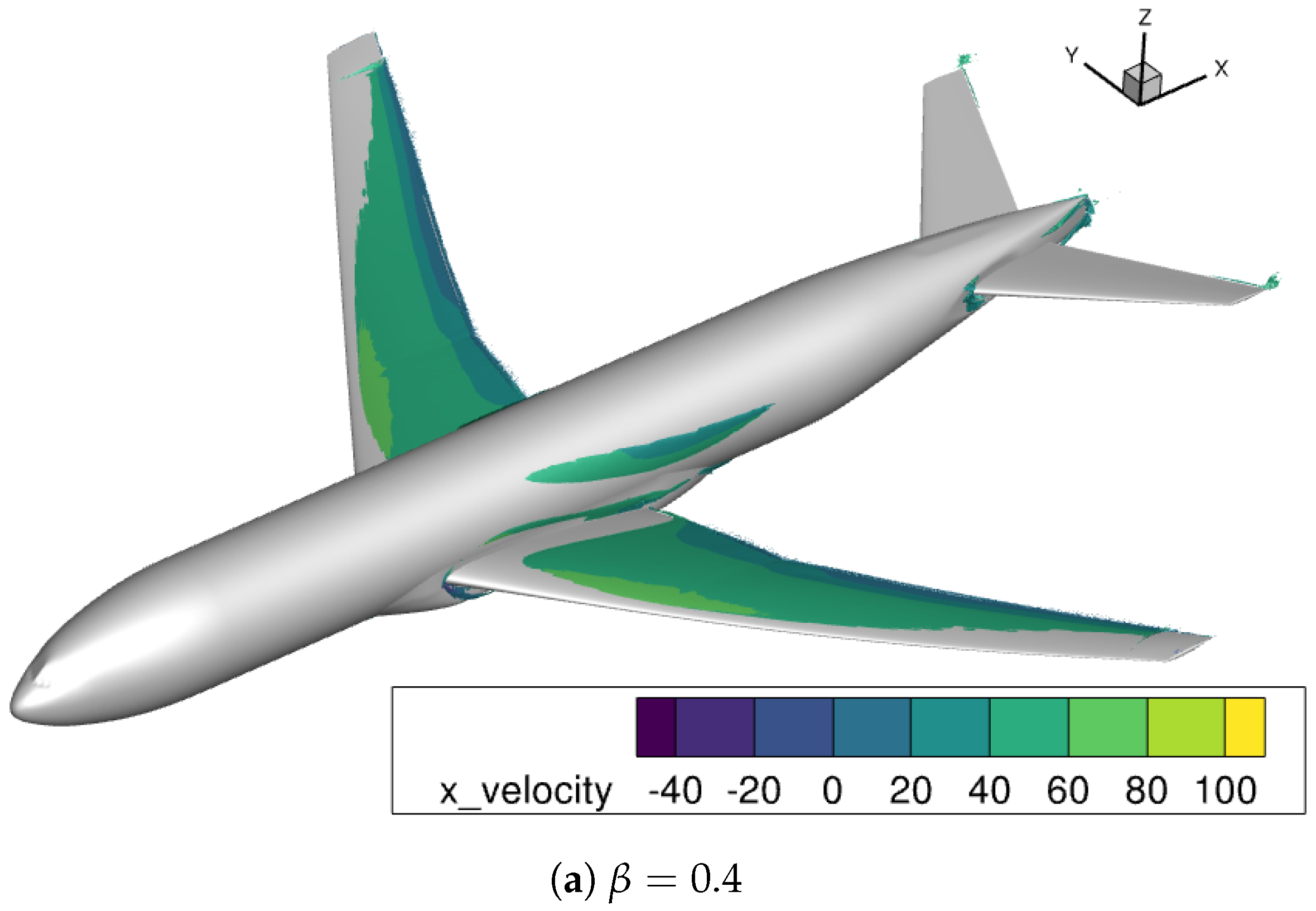
4.1. Test Case: NASA Common Research Model

The present study considers the NASA Common Research Model (CRM) with horizontal tailplanes (HTP) as a 3D test case to investigate the applicability of the 2D-based model augmentation. The model does not include high-lift devices nor nacelles. The target flow configuration is a Mach number M a = 0.25 and a Reynolds number R e = 17 × 10 6 , which is selected from the ESWIRP (European Strategic Wind Tunnels Improved Research Potential) wind tunnel campaign conducted at the European Transonic Windtunnel (ETW) in 2014 [26]. Experimental data from the ESWIRP test campaign are publically available. The experimental pressure coefficients that are shown later against our CFD results are taken from the Polar 251 dataset.
Figure 9 shows the measured lift coefficient curve over angles of attack. As can be seen, there is a clear indication of stall at around α = 12.5 deg. We focus our study on the pre-stall regime at two angles of attack, α = 10.92 deg and α = 12.35 deg. At both angles of attack, the flow over the main wing should not be separated in the experiment, but a relatively large adverse pressure gradient is present, which we expect would lead to a certain degree of model correction when using the augmented SA-neg model.
Simulations were performed using the baseline SA-neg model and the augmented SA-neg model. Note that the augmented SA-neg model is used without the sensor function. As the flow remains attached on large parts of the wing, the augmentation should be applied almost on the entire wing surface, i.e., the situation with the sensor is expected to be similar to the 2D airfoil HGR-01 for an incidence angle smaller than 10 deg. The attached boundary layer is subjected to a strong adverse pressure gradient, and hence, the model augmentation is activated.
Figure 10 shows the overview of the computational grid used in this study. The baseline grid is a fine solar grid from the Fourth AIAA Drag Prediction Workshop (DPW-IV) [27], which has approximately 34.1 million points. This preexisting mesh also takes into account the experimentally measured deformation of the main wing at α = 14 deg. Although this is slightly mismatched with the angles of attack ( α = 10.92 deg, α = 12.35 deg) considered in this study, the overall lift load causing this deformation is not very different (cf. Figure 9) and, therefore, should lead to comparable deformations. Thus, the authors think that this potential mismatch can be considered negligible compared to the turbulence-modeling effects and does not affect our main conclusions drawn in this study.

4.2. Results

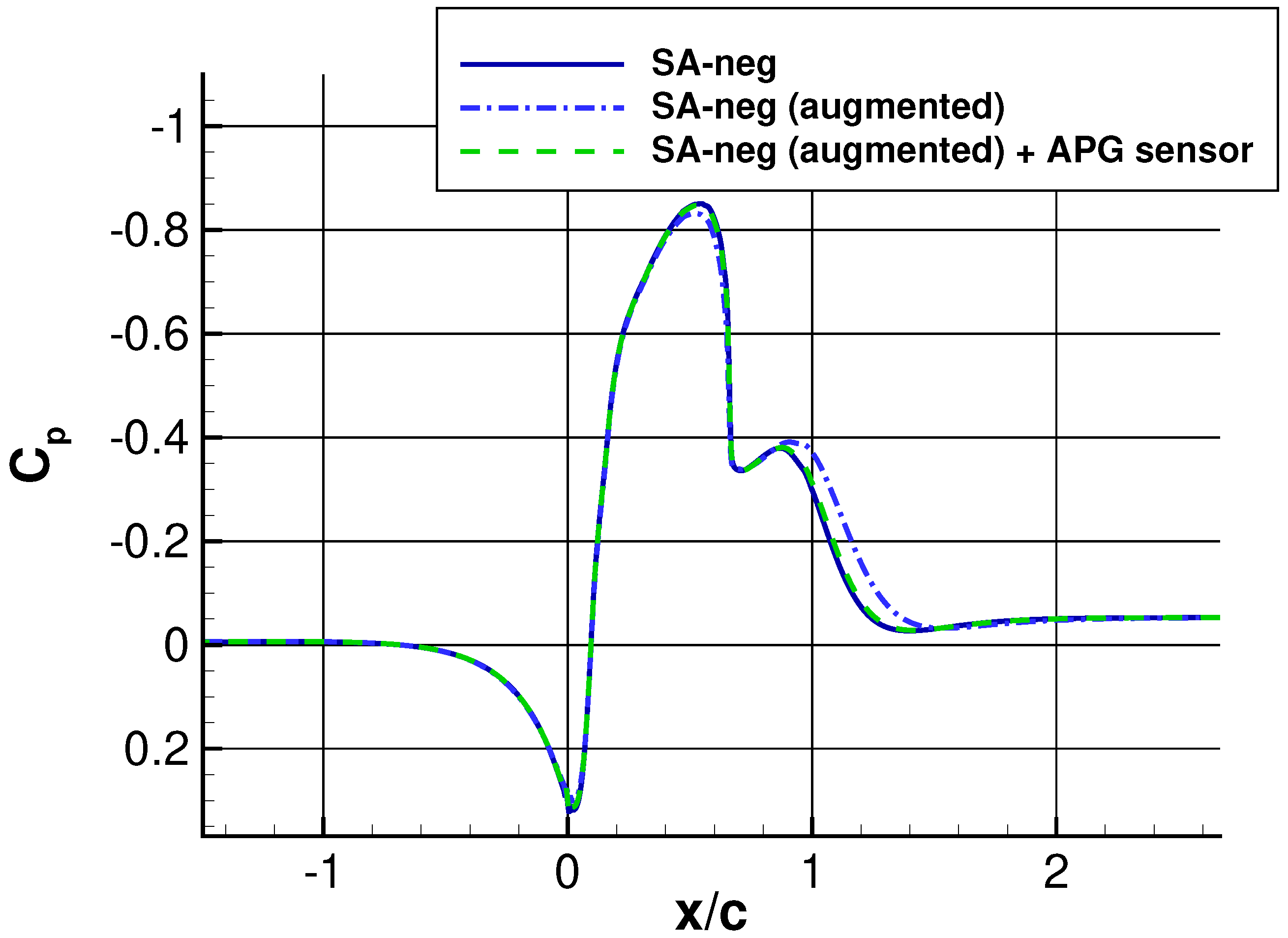
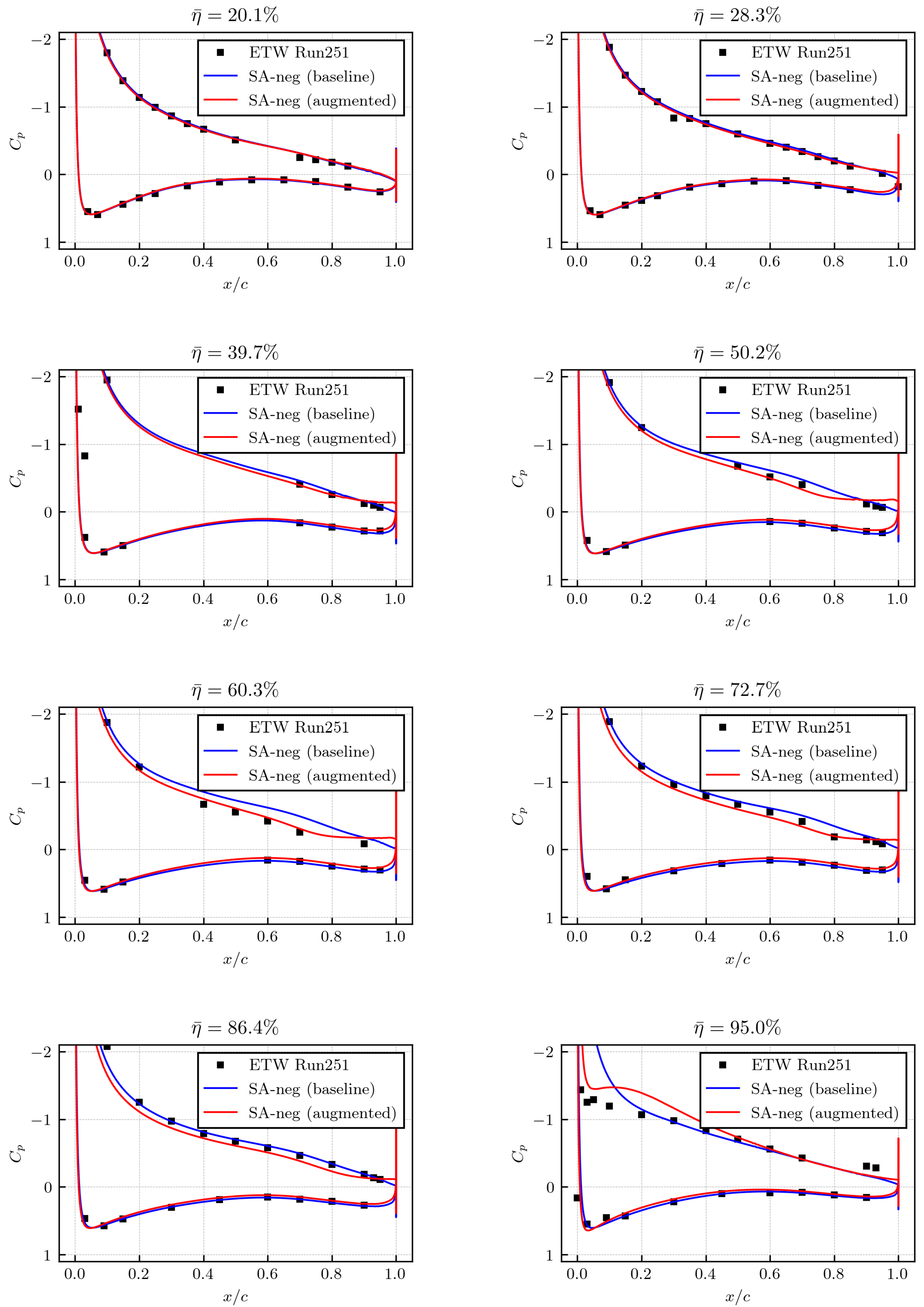
4.2.1. Pressure Coefficients

Figure 11 and Figure 12 show the predictions of the pressure coefficient over the main wing simulated by the baseline SA-neg model and the augmented SA-neg model at each incidence angle. As expected, the baseline model already shows good agreement with the experimental data for both angles of attack since these are below the stall regime. Moreover, the overall differences between the baseline model and the augmented model are relatively small, especially in the inboard area (i.e., small non-dimensionalized spanwise location η ¯ ), and slightly larger in the outboard area. Here, the spanwise coordinate η ¯ = y / B , B is the wing span, and hence, η ¯ = 0 at the wing root and η ¯ = 1 at the wing tip. Moreover, note that the notation of η ¯ used traditionally in aircraft aerodynamics should not be confused with the flow features η 1 , η 2 , η 3 used in the augmented turbulence model. In addition, the model correction is, as predicted, larger at the higher incidence angle due to a greater adverse pressure gradient. Especially at α = 12.35 deg, the augmented model seems to give some improvement around η ¯ = 60.3 %.
Notable differences are observed at η ¯ = 95 % of the α = 12.35 deg case. While the baseline model preserves a clear suction peak, the augmented model shows a suction drop near the leading edge, which is also present in the experimental data, and a following short plateau, which is, however, not seen in the experiment. Visualizations of streamlines projected onto the X-Z plane in Figure 13 suggest that these effects are due to a local separation bubble that is only obtained with the augmented model. Although separation is also the likely reason for the suction drop in the experiment, the deviations in c p at x / c 0.2 , as well as near the trailing edge, suggest a somewhat different pattern than predicted by the augmented model. Still, some improvement with respect to c p compared to the fully attached flow prediction by the baseline model can be stated.

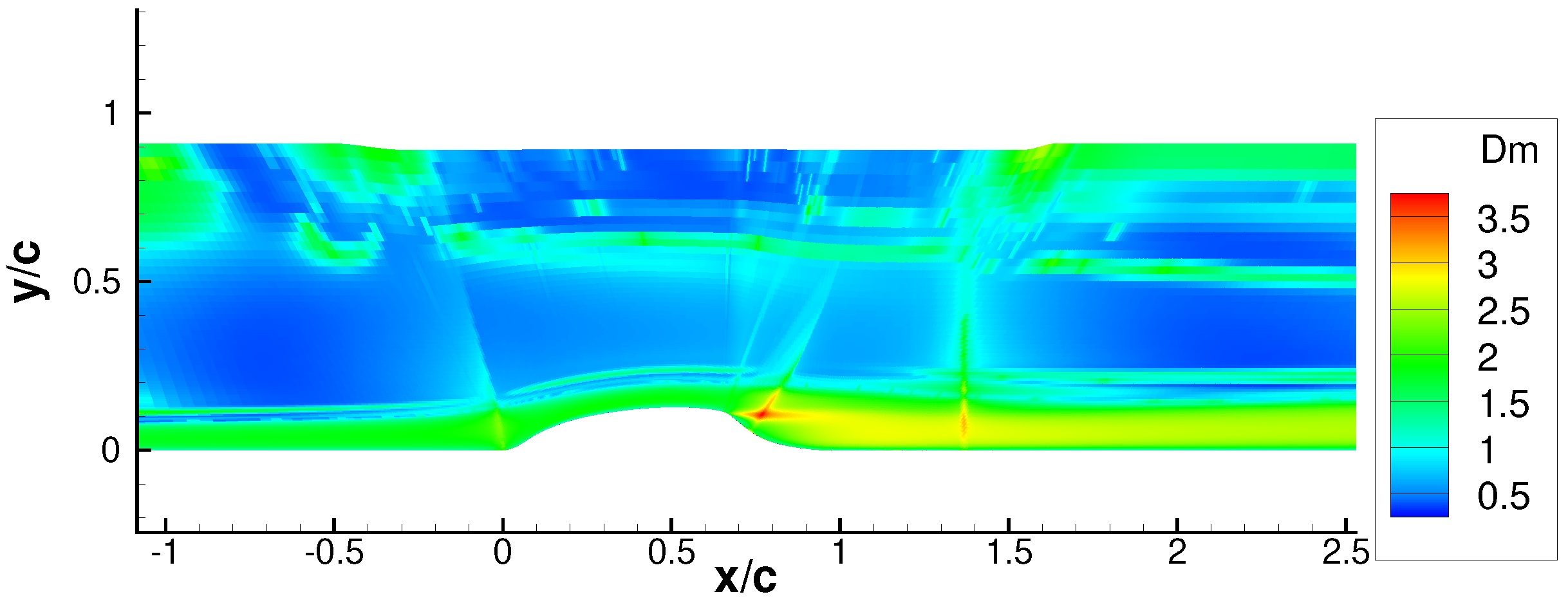
4.2.2. Model Correction Fields

Figure 14 and Figure 15 show the iso-surfaces of the correction field β at each incidence angle. For each iso-surface of two different values, β = 0.4 and β = 0.8 are visualized. It should be recalled that the value β = 1.0 means that no model correction is introduced, and the smaller the value is, the stronger the model correction is. Hence, relatively strong model corrections are visualized by the iso-surface β = 0.4 , and relatively mild corrections by β = 0.8 . For both angles of attack, the β = 0.4 iso-surface is mainly restricted to the main wing, which is subjected to an adverse pressure gradient. Although the augmented model is trained for 2D airfoil flows and the present case is a 3D-flow, the majority of the flow over the main wing should be close to two-dimensional at these incidence angles. Therefore, the flow features used in the 2D training are still considered to be valid and are responding to the adverse pressure gradient flow. In fact, as illustrated in Figure 16, the correction field clearly resembles that of 2D airfoil cases, such as the HGR-01 case when looking at the η ¯ = 60.3 % spanwise location for the α = 12.35 deg case. These observations suggest that the data-driven model correction inferred from the 2D dataset could partly be usable in the nearly 2D-flow regime of a 3D-flow configuration. On the other hand, the β = 0.8 iso-surface not only surrounds almost the entire wings and fuselage, but is also present in a few regions where the flow should be highly three-dimensional (e.g., wing tips, wing–body juncture). Since the model correction is not trained for such highly three-dimensional flows, the prediction accuracy could potentially be harmed as the machine learning model is certainly extrapolating in such a scenario. To avoid this, an ad hoc treatment by a similar sensor-based approach is required in the 2D case, or more insights from a complete 3D training might be necessary.

5. Conclusions

The generalizability of a data-augmented Spalart–Allmaras turbulence model trained via the field inversion and machine learning strategy was studied for two-dimensional (2D) and three-dimensional (3D) aerodynamic flow cases. Throughout this paper, we focused on one data-driven model with a closed-form expression that was trained for 2D separated airfoil flows [8] in order to be consistent with the model and to have good interpretability of the results.
In 2D-flow cases, while consistent improvements are observed in the airfoil flows, the model corrections inferred from the embedded machine learning model could negatively affect the prediction of the other flows, as shown in the NASA hump case. Using a common machine learning terminology, one can say that the considered model augmentation is “over-fitted” to the airfoil flow configurations. The detrimental effect of the data-driven model corrections observed in the NASA hump case is a typical example of extrapolation, meaning that the machine learning model is applied to the outside of the scope of training data, and hence, its prediction has high uncertainty. To prevent the unwanted model corrections, we introduced a set of sensor functions to localize the model corrections. With this approach, the model is corrected only inside the attached boundary layer with an adverse pressure gradient. While the sensor works as a limiter or an additional “safety net” to preserve the predictive capability of the baseline model for non-airfoil flows, much of the improvement for the airfoil flows at high incidence angles was lost due to the deactivation of the model augmentation inside the separated shear layers. Nevertheless, the data augmentation with physics-based sensors could offer a compromised model, which provides improvement for target flow phenomena while not losing the predictive capability of the baseline model at worse.
Furthermore, the augmented model was applied to a 3D aircraft flow configuration, the NASA Common Research Model (CRM) with horizontal tail-planes. This should be seen as a preliminary exercise to investigate the generalizability of the 2D-based augmentation to 3D flows. The data-augmented model produced similar predictions of the pressure coefficients over the main wing to the baseline model with indications of some improvement, especially for the higher incidence angle. The investigation of the correction field revealed that relatively strong model corrections were restricted to the main wing subjected to an adverse pressure gradient. In those regions, the flow should be close to two-dimensional, and therefore, the features used in the 2D training are still considered to be valid. On the other hand, relatively weak corrections are active in the majority of the near wall regions, and a few regions where the flow should be highly three-dimensional (e.g., wing tips, wing–body juncture). The latter could be harmful, and thus an ad hoc treatment by a similar sensor-based approach is required in the 2D case, or more insights from a complete 3D training might be necessary.
It is obvious that further studies are required towards achieving a more generalizable model augmentation for 2D adverse pressure gradient flows with separation. As discussed in the present study, the different modeling focuses between airfoil flows and the NASA hump-like flows should be taken into account for this purpose. Also, future work in 3D-flows may include investigations on the post-stall regime of a 3D aircraft flow, which could not be covered in the present work.

Author Contributions

Conceptualization, Y.N., C.G., A.P., A.K. and T.K.; methodology, Y.N. and T.K.; software, Y.N.; validation, Y.N.; formal analysis, Y.N.; investigation, Y.N.; resources, Y.N., T.K. and A.K.; data curation, Y.N. and A.K.; writing—original draft preparation, Y.N.; writing—review and editing, A.P., A.K., T.K. and C.G.; visualization, Y.N. and A.K.; supervision, A.P. and A.K.; project administration, A.K.; funding acquisition, C.G. and A.K. All authors have read and agreed to the published version of the manuscript.

Funding

The funding of the presented work within the Luftfahrtforschungsprogramm VI-1 (LUFO VI-1) project SMARTfly (SMARTfly—Smart Modeling of flying Transport Vehicles—Entwicklung exakter und effizienter Modellierungen und Simulationsmethoden für den Entwurf von Fluggeräten und Triebwerken, FKZ: 20X1909A) by the German Federal Ministry for Economic Affairs and Climate Action (BMWK) is gratefully acknowledged. The funding of this work by the DLR internal aeronautical program within the project ADaMant is also gratefully acknowledged.

Data Availability Statement

The simulation data are stored on DLR premises and are not publicly accessible. Processed data could be made available upon request. This requires permission by DLR.

Acknowledgments

The authors are grateful to our colleague Stefan Keye for providing the computational grid of the NASA CRM test case.

Conflicts of Interest

The authors declare no conflicts of interest.

References

  1. Cary, A.W.; Chawner, J.; Duque, E.P.; Gropp, W.; Kleb, W.L.; Kolonay, R.M.; Nielsen, E.; Smith, B. CFD Vision 2030 Road Map: Progress and Perspectives. In Proceedings of the AIAA Aviation 2021 Forum, Virtual, 2–6 August 2021. [Google Scholar] [CrossRef]
  2. Weatheritt, J.; Sandberg, R. A novel evolutionary algorithm applied to algebraic modifications of the RANS stress–strain relationship. J. Comput. Phys. 2016, 325, 22–37. [Google Scholar] [CrossRef]
  3. Schmelzer, M.; Dwight, R.P.; Cinnella, P. Discovery of Algebraic Reynolds-Stress Models Using Sparse Symbolic Regression. Flow Turbul. Combust. 2020, 104, 579–603. [Google Scholar] [CrossRef]
  4. Ling, J.; Kurzawski, A.; Templeton, J. Reynolds averaged turbulence modelling using deep neural networks with embedded invariance. J. Fluid Mech. 2016, 807, 155–166. [Google Scholar] [CrossRef]
  5. Singh, A.P.; Duraisamy, K. Using field inversion to quantify functional errors in turbulence closures. Phys. Fluids 2016, 28, 045110. [Google Scholar] [CrossRef]
  6. Cherroud, S.; Merle, X.; Cinnella, P.; Gloerfelt, X. Space-dependent Aggregation of Stochastic Data-driven Turbulence Models. arXiv 2024, arXiv:2306.16996. [Google Scholar]
  7. Srivastava, V.; Rumsey, C.L.; Coleman, G.N.; Wang, L. On Generalizably Improving RANS Predictions of Flow Separation and Reattachment. In Proceedings of the AIAA Scitech 2024 Forum, Orlando, FL, USA, 8–12 January 2024. [Google Scholar] [CrossRef]
  8. Jäckel, F. A Closed-Form Correction for the Spalart–Allmaras Turbulence Model for Separated Flows. AIAA J. 2023, 61, 2319–2330. [Google Scholar] [CrossRef]
  9. Allmaras, S.R.; Johnson, F.T. Modifications and clarifications for the implementation of the Spalart-Allmaras turbulence model. In Proceedings of the Seventh International Conference on Computational Fluid Dynamics (ICCFD7), Big Island, HI, USA, 9–13 July 2012; Volume 1902. [Google Scholar]
  10. Holland, J.R.; Baeder, J.D.; Duraisamy, K. Field Inversion and Machine Learning with Embedded Neural Networks: Physics-Consistent Neural Network Training. In Proceedings of the AIAA Aviation 2019 Forum, Dallas, TX, USA, 17–21 June 2019. [Google Scholar] [CrossRef]
  11. Somers, D.M. Design and Experimental Results for the S809 Airfoil. Technical Report. 1997. Available online: https://www.osti.gov/biblio/437668/ (accessed on 30 May 2024).
  12. Wokoeck, R.; Krimmelbein, N.; Ortmanns, J.; Ciobaca, V.; Radespiel, R.; Krumbein, A. RANS Simulation and Experiments on the Stall Behaviour of an Airfoil with Laminar Separation Bubbles. In Proceedings of the 44th AIAA Aerospace Sciences Meeting and Exhibit, Reno, NV, USA, 9–12 January 2006. [Google Scholar] [CrossRef]
  13. Schwamborn, D.; Gerhold, T.; Heinrich, R. The DLR TAU-Code: Recent Applications in Research and Industry. In Proceedings of the European Conference on Computational Fluid Dynamics, ECCOMAS CFD 2006, Delft, The Netherlands, 5–8 September 2006. [Google Scholar]
  14. Brezillon, J.; Dwight, R. Discrete Adjoint of the Navier-Stokes Equations for Aerodynamic Shape Optimization. In Proceedings of the EUROGEN 2005—Sixth Conference on Evolutionary and Deterministic Methods for Design, Optimization and Control with Applications to Industrial and Societal Problems, Munich, Germany, 2–14 September 2005. [Google Scholar]
  15. Bekemeyer, P.; Bertram, A.; Chaves, D.A.H.; Ribeiro, M.D.; Garbo, A.; Kiener, A.; Sabater, C.; Stradtner, M.; Wassing, S.; Widhalm, M.; et al. Data-Driven Aerodynamic Modeling Using the DLR SMARTy Toolbox. In Proceedings of the AIAA AVIATION 2022 Forum, Chicago, IL, USA, 27 June–1 July 2022. AIAA 2022-3899. [Google Scholar] [CrossRef]
  16. Paszke, A.; Gross, S.; Massa, F.; Lerer, A.; Bradbury, J.; Chanan, G.; Killeen, T.; Lin, Z.; Gimelshein, N.; Antiga, L.; et al. PyTorch: An Imperative Style, High-Performance Deep Learning Library. arXiv 2019, arXiv:1912.01703. [Google Scholar]
  17. Eisfeld, B. The importance of turbulent equilibrium for Reynolds-stress modeling. Phys. Fluids 2022, 34, 025123. [Google Scholar] [CrossRef]
  18. Nishi, Y.; Knopp, T.; Probst, A.; Grabe, C.; Krumbein, A. Towards local application oF data-driven turbulence modeling for separated flows. In Proceedings of the 14th International ERCOFTAC Symposium on Engineering, Turbulence, Modelling and Measurements, ETMM14, Barcelona, Spain, 6–8 September 2023. [Google Scholar]
  19. Ling, J.; Kurzawski, A. Data-driven Adaptive Physics Modeling for Turbulence Simulations. In Proceedings of the 23rd AIAA Computational Fluid Dynamics Conference, Denver, CO, USA, 5–9 June 2017. [Google Scholar] [CrossRef]
  20. Knopp, T.; Reuther, N.; Novara, M.; Schanz, D.; Schülein, E.; Schröder, A.; Kähler, C.J. Modification of the SSG/LRR-Omega Model for Turbulent Boundary Layer Flows in an Adverse Pressure Gradient. Flow Turbul. Combust. 2023, 111, 409–438. [Google Scholar] [CrossRef]
  21. Naughton, J.W.; Viken, S.; Greenblatt, D. Skin Friction Measurements on the NASA Hump Model. AIAA J. 2006, 44, 1255–1265. [Google Scholar] [CrossRef]
  22. Alaya, E.; Grabe, C.; Eisfeld, B. Evolutionary Algorithm applied to Differential Reynolds Stress Model for Turbulent Boundary Layer subjected to an Adverse Pressure Gradient. In Proceedings of the AIAA AVIATION 2022 Forum, Chicago, IL, USA, 27 June–1 July 2022. [Google Scholar] [CrossRef]
  23. Speziale, C.G.; Sarkar, S.; Gatski, T.B. Modelling the pressure–strain correlation of turbulence: An invariant dynamical systems approach. J. Fluid Mech. 1991, 227, 245–272. [Google Scholar] [CrossRef]
  24. Yacine Bentaleb, S.L.; Leschziner, M.A. Large-eddy simulation of turbulent boundary layer separation from a rounded step. J. Turbul. 2012, 13, N4. [Google Scholar] [CrossRef]
  25. Ling, J.; Templeton, J. Evaluation of machine learning algorithms for prediction of regions of high Reynolds averaged Navier Stokes uncertainty. Phys. Fluids 2015, 27, 085103. [Google Scholar] [CrossRef]
  26. Boyet, G. ESWIRP: European strategic wind tunnels improved research potential program overview. Ceas Aeronaut. J. 2018, 9, 249–268. [Google Scholar] [CrossRef]
  27. Vassberg, J.; Tinoco, E.; Mani, M.; Rider, B.; Zickuhr, T.; Levy, D.; Brodersen, O.; Eisfeld, B.; Crippa, S.; Wahls, R.; et al. Summary of the Fourth AIAA CFD Drag Prediction Workshop. In Proceedings of the 28th AIAA Applied Aerodynamics Conference, Chicago, IL, USA, 28 June–1 July 2010. [Google Scholar] [CrossRef]
Figure 1. The workflow of the FIML.
Aerospace 11 00592 g001
Figure 2. Skin friction coefficient on the NASA wall-mounted hump. Results of the Speziale–Sarkar–Gatski (SSG) Reynolds stress model and its data-enhanced model by gene-expression programming (SSG-GEP) in [22] are also shown for comparison.
Aerospace 11 00592 g002
Figure 3. Mahalanobis distance metric on the NASA hump case evaluated for the augmented SA-neg model.
Aerospace 11 00592 g003
Figure 4. Comparison of the β -fields between global (a) and local (b) model augmentation for the NASA hump.
Aerospace 11 00592 g004
Figure 5. Pressure coefficient c p on the NASA hump case. Note that the vertical axis is reversed.
Aerospace 11 00592 g005
Figure 6. Lift coefficient vs. angle of attack.
Aerospace 11 00592 g006
Figure 7. Comparison of the β -fields between global (a) and local (b) model augmentation at incidence angle α = 12 deg.
Aerospace 11 00592 g007
Figure 8. Wall profiles at x / c = 0.5 for the local model augmentation, α = 12 deg.
Aerospace 11 00592 g008
Figure 9. Measured lift coefficient vs. angle of attack at the ESWIRP ETW test campaign.
Aerospace 11 00592 g009
Figure 10. Overview of the NASA CRM mesh.
Aerospace 11 00592 g010
Figure 11. Prediction of the pressure coefficients over the main wing at different spanwise locations for the incidence angle α = 10.92 deg. Note that η ¯ represents the non-dimensionalized spanwise location ( η ¯ = 100 % at the wing tip).
Aerospace 11 00592 g011
Figure 12. Prediction of the pressure coefficients over the main wing at different spanwise locations for the incidence angle α = 12.35 deg. Note that η ¯ represents the non-dimensionalized spanwise location ( η ¯ = 100 % at the wing tip).
Aerospace 11 00592 g012
Figure 13. Comparison of the flow field at the spanwise location η ¯ = 0.95 for α = 12.35 deg colored by Mach number. Streamlines projected onto the X-Z plane are shown together.
Aerospace 11 00592 g013
Figure 14. Iso-surfaces of the model correction field β for α = 10.92 deg colored by the streamwise velocity.
Aerospace 11 00592 g014
Figure 15. Iso-surfaces of the model correction field β for α = 12.35 deg colored by the streamwise velocity.
Aerospace 11 00592 g015aAerospace 11 00592 g015b
Figure 16. The correction field β at spanwise location η ¯ = 60.3 % for α = 12.35 deg.
Aerospace 11 00592 g016
Table 1. Summary of the training cases and the flow conditions used in [8], including the Mach numbers M a , Reynolds numbers R e , angles of attack α , and reference data.
Test Case Ma Re α [deg]Reference Data
S8090.1 2 × 10 6 8.2, 16.24 c p [11]
HGR-010.07 0.65 × 10 6 13.7 c l [12]
RAE28220.721 8.79 × 10 6 5.67 c p
Disclaimer/Publisher’s Note: The statements, opinions and data contained in all publications are solely those of the individual author(s) and contributor(s) and not of MDPI and/or the editor(s). MDPI and/or the editor(s) disclaim responsibility for any injury to people or property resulting from any ideas, methods, instructions or products referred to in the content.

