Article

Optimization Study of Steady-State Aerial-Towed Cable Circling Strategy Based on BP Neural Network Prediction

by
Luqi Feng
,
Xueqiang Liu
* and
Zi Feng Nio
College of Aerospace Engineering, Nanjing University of Aeronautics and Astronautics, Nanjing 210016, China
*
Author to whom correspondence should be addressed.
Aerospace 2024, 11(7), 594; https://doi.org/10.3390/aerospace11070594
Submission received: 25 May 2024 / Revised: 3 July 2024 / Accepted: 19 July 2024 / Published: 21 July 2024
(This article belongs to the Special Issue Aerodynamic and Multidisciplinary Design Optimization)

Abstract

:
This paper presents models for UAV aerial-towed cables in free-end and fixed-end configurations, crucial for tasks like communication and aerial charging. By establishing a quasi steady-state model, computational results on cable shapes are obtained. To accelerate computations, a backpropagation (BP) neural network prediction model is trained, significantly reducing the computation time. An evaluation function has been developed that integrates both aircraft performance and cable shape considerations to evaluate circling parameters across various states. This function integrates techniques such as BP neural networks and particle swarm optimization (PSO) to refine parameters such as velocities and bank angles for both free-end and fixed-end cables. The results show that the BP neural network accurately predicts cable shapes, achieving a maximum error of 5% in towing force and verticality. Additionally, PSO efficiently optimizes circling parameters, thereby enhancing the effectiveness of the evaluation function in identifying optimal solutions. This approach significantly improves the efficiency of determining optimal circling parameters for UAV aerial-towed cables, thereby contributing to their operational efficacy.

1. Introduction

The growing use of large UAVs has drawn more attention to technologies like UAV aerial relay communication and UAV aerial charging, leading to the progressive expansion and heightened interest in application scenarios for UAV aerial-towing cables. When the circling altitude, velocity and bank angle parameters of the orbiting aircraft are determined, its orbit is fixed, the shape of the towing cable tends to be stabilized, and its parameters will be able to be derived via calculation. At present, several organizations or individuals have proposed numerical methods for the aerial-towed cable structure under circling state [1].
Ma et al. [2] from Beijing University of Aeronautics and Astronautics (BUAA) used the lumped mass method to simulate the kinematic state of a rear-towed antenna in a stable circling state, which improved the computational accuracy. Furthermore, the authors found that the effect of velocity on the verticality of the cable was more sensitive, whereas the drogue’s mass has lower sensitivity with the change in verticality. Ma et al. [3] used the tension recurrence method to analyze the aerial-towed decoy system to improve the computational efficiency; the fast corresponding prediction of the aerial-towed decoys in an adequate time became possible and proved the effectiveness of the method.
Zhu [4] established a multi-body dynamics model for cable towing to analyze the cable-towing system during aircraft circling. The numerical results from this model are similar to the numerical computations using the finite elemental method under the same conditions. The simulation results showed that in order to maintain the required verticality within a specified range, it is advisable to reduce the aircraft velocity appropriately under similar conditions. This adjustment is necessary to fulfill operational specifications. Merz and Johansen studied the feasibility of a circularly towed cable-body system for UAV applications. The author used a lumped parameter model for the circular towed cable-body system analysis and optimized the system to obtain the optimal control strategy in the process of UAV towing and circling. The results show that an increase in the length of the cable will reduce the radius of the end of the cable, while at the same time, the orbiting aircraft’s circling radius positively correlates with the circling radius at the end of the cable. Nevertheless, when controlling the shape of the cable, it is essential to consider the aerodynamic performance of the towed carrier itself [5,6]. Williams and Trivailo investigated a circularly towed-cable system with an attached windsock. The authors employed an improved system with a discretized lumped mass model of the cable for numerical analysis. The study indicates that the radius of the towed body can be enhanced by incorporating a drag device. Nevertheless, the increased complexity resulting from installing such a device may outweigh the potential benefits [7]. Murray proposed using the concept of differential flatness to handle the towed cable-body system. This approach simplifies trajectory generation by transforming a high-dimensional dynamic optimization problem into a low-dimensional nonlinear optimization problem. Consequently, this method significantly reduces the computational workload [8]. In terms of UAV aerial docking, Wang et al. proposed the use of a drogue in the aerial recharging method for small UAVs. The study involved investigating the aerial docking of drones and conducting on-site flight tests to discuss the feasibility of this approach [9].
The verticality of the towing cable affects its working efficiency, and if the verticality of the towing cable is lower than 70%, its working performance will be affected [10]. Under the current research direction, researchers have been able to simulate and calculate the shape parameters of the tethered cable under different operating conditions using the simplified finite element method, which shows that the increase in the cable length and the decrease in the aircraft’s circling velocity can increase the verticality of the cable, and at the same time, the decrease in the aircraft’s circling radius can also optimize the circling radius of the end of the cable [2,11]. However, in the actual working process, the circling maneuver of the aircraft will lead to a decrease in its aerodynamic efficiency; not only will the stall speed increase, but also the circling bank angle will be limited, due to factors such as vibration or structural overload. Furthermore, the longer cable will also produce a larger drag force, which will inevitably have an impact on the circling state of the aircraft. Therefore, the key to this technology lies in how to determine the circling parameters of the orbiting aircraft so that it can meet the towed cable working needs as much as possible without affecting the aerodynamic performance of the carrier.
Although it has been simplified in many aspects, it still takes a lot of time to calculate the circularly towed cable parameters and optimize them if they are calculated directly using numerical methods, and therefore there is a need to find fitting algorithms that can make predictions based on the available data quickly [12,13]. This article first establishes a quasi-static model of the towed-cable system and analyzes the parameters affecting the verticality, towing force and cable end circling range of the towed-cable system during the steady-state hovering phase of the carrier. A certain amount of the steady-state towing system dataset is obtained through calculation and analysis. Using this as the training sample, the BP neural network is employed for prediction training, significantly reducing the parameter calculation time of the steady-state towing system. Finally, an evaluation function for the performance of the steady-state towing cable system is proposed, and the PSO algorithm is used to search for the optimal value of the evaluation function within a certain range. The final study shows that the multi-hidden layer BP neural network can effectively predict the parameters of the steady-state circling towed cable; the evaluation function proposed in this paper can be adapted to the towed-cable system and the PSO algorithm can be used to find the optimal solution of the evaluation function with high efficiency.

2. Modeling and Calculation Methods

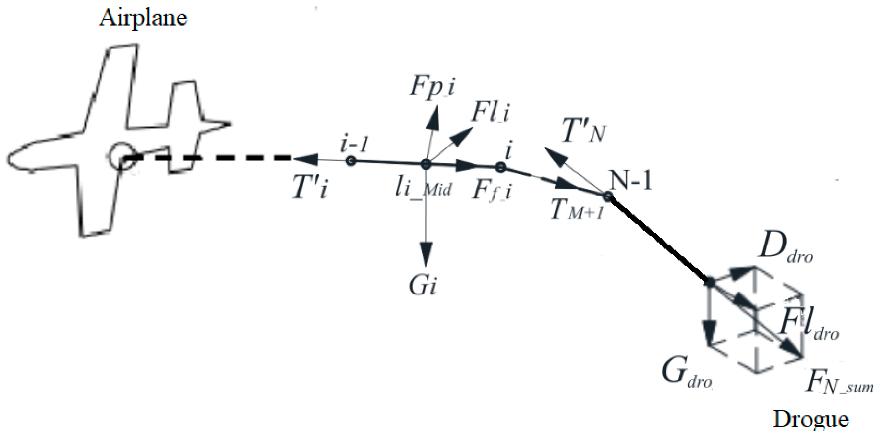
2.1. Steady-State Trailing Cable Model

2.1.1. Quasi-Stationary Circling Aircraft Model for Unconstrained Trailing Cable

In the circular towing process, as the circling trajectory of the aircraft remains constant, the spatial shape of the towing cable gradually stabilizes. This stabilization serves as the foundation for establishing the quasi-static model of the towed antenna system. Neglecting the minor factors, in order to simplify the calculations to some extent without affecting the results of the calculations, this study made the following assumptions:
  • The towing cable is considered a flexible structure that exhibits high flexibility while maintaining inextensible.
  • The aircraft maintains a constant altitude while circling uniformly.
  • This paper mainly considers the circling of a towed carrier in a stabilized environment. The wind speed profile in the environment is not taken into consideration, and only the relative wind speed in the circling is taken into account as one of the variables.
  • In the following section, the computational results of the model in this paper will be verified against the existing literature to verify that the assumptions made in paper do not affect the computational results.
The antenna is set to be in a stable circling state, and the cable is stabilized. The origin O is the circling center, the Z-axis is vertical, the X-axis is parallel to the horizontal plane and the Y-axis satisfies the right-hand rule. The circling plane XOY is determined by the flight altitude H of the carrier aircraft and the steady-state circling radius R is expressed as follows:
R 0 = V t r u e 2 g | tan φ |
where φ is the bank angle, g is the g ravity acceleration and Vtrue is the true airspeed.
Figure 1 show the model of the towed-cable system with unconstrained end. First, the cable system is discretized into fixed-length rigid rod microsegments connected at the head and tail. Then, any point below the flight altitude and within the circling radius as the coordinates of the drogue was selected, combined with the centrifugal force, the aerodynamic force and the gravity force of the drogue, and then, according to Newton’s third law, the tension T n of the end segment of the cable and its direction vector l n were determined. According to the backward deduction of the N − 1 tail coordinates of the microsegment and the circling radius Rn−1, the aerodynamic force of the cable was added, and then the magnitude and direction of the tension were iteratively corrected. By analogy, the magnitude and direction of the tension in each of the other segments of the cable were obtained. Finally, the deviation △R and △H between the radius and altitude of the first microsegment (i.e., towing point) and the given flight conditions were compared; the drogue’s coordinates N were adjusted and iterated until the residual error converged. The tension T i recurrence relationship is as follows:
{ T i = ( m i g + F l i + F q i + D d r o ) ( i = N ) T i = T i + 1 m i g F l i F q i ( 1 i < N )
where mi, F l i , F q i denote the mass, centrifugal force and aerodynamic force of microsegment i, respectively, and D d r o denotes the drogue’s drag force. The solution equations are as follows, respectively:
{ F l i = m i ω 2 R i n L n F q i = F p i + F f i D d r o = 1 2 ρ V n 2 C d r o A
where, ω denotes the circling angular velocity, which is equal everywhere because the towed-cable system is in the proposed steady state. F q i , F p i and F f i denote the total aerodynamic force, differential pressure force, and friction force of the i-th microsegment, V n is the velocity of the drogue (n-th microsegment). ρn, Cdro and A represent the air density, drag coefficient, and the area of the drogue, respectively. Those formulas for any rod may be derived as follows:
{ F p i = C p 1 2 ρ | V n i | V n i d l F f i = C f 1 2 ρ | V t i | V t i 2 π r l
where, V n i and V t i indicate the normal velocity and tangential velocity of microsegment i, respectively. Cp and Cf indicate the pressure drag coefficient and friction coefficient of the cable segments, respectively. The values of Cp and Cf are 0.1 and 0.02, respectively.
The calculation method in this paper is essentially an inverse calculation method, which firstly calculates the force at the end of the cable, and then, based on aerodynamics and Newton’s laws, reverse engineers the cable’s state at other positions. It iteratively adjusts the endpoint until the cable shape meets the requirements. A simplified flow chart of the model calculation is shown in the following Figure 2:

2.1.2. Quasi-Stationary Circling Aircraft Model for Fixed-End Trailing Cable

This paper focuses on simulation optimization for two application scenarios, a UAV towing cable and UAV aerial charging. Therefore, it is necessary to consider two working states, the free-end condition and the fixed-end condition [14]. The structure of the towing cable in the fixed-end condition is similar to the free-end condition; the force on the end section of the cable is first calculated using Newton’s law and then the aerodynamic force on the end section is changed to the reaction force on the cable from the fixed point, which is not constant and will change with the change in the cable structure. By constantly changing the end force and cable length, the cycle is iterated until the first section of the cable position meets the requirements.The cable schematic is shown in Figure 3.
The tension T i of the discrete sections of the cable under the end fixation is as follows:
{ T i = ( m i g + F l i + F q i + F dro ) ( i = N ) T i = T i + 1 m i g F l i F q i ( 0 < i < N )

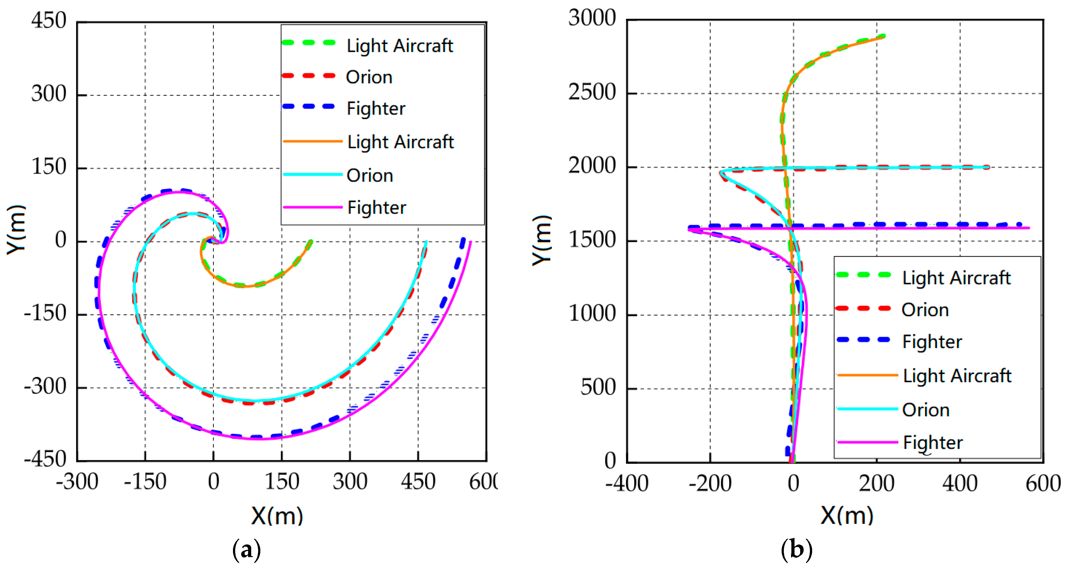
2.1.3. Model Accuracy Validation

To validate the accuracy of the model, the verticality of the TACAMO system’s antenna is computed using system parameters extracted from the literature [11]. Verticality is defined as the ratio of the total length of the towing cable to the amount of sagging observed during the circling maneuver. Typically, this ratio is a value less than 1 or as a percentage.
The comparison of the verticality reveals a reasonably consistent outcome between the calculations, with a maximum deviation of approximately 5.85%. In Table 1, Verticality (V1) represents the referenced values, while Verticality (V2) denotes the obtained values, revealing minor errors upon analysis.
In addition to calculating the verticality of the towing cable and towing force, this paper uses a calculation model to verify the cable’s spatial shape. The model’s parameters are referenced from the results in the literature [7]. The fundamental parameters of the towing cable include the following: the density ρ = 970 kg/m3, the length of the cable L = 3000 m, the drogue’s mass md = 10 kg and the drag characteristics of the drogue at the end of the cable Cdro = 2.0 m2; other parameters are shown in the following Table 2:
Figure 4 illustrates the comparison between simulated data and data sourced from the existing literature [7]. The dotted lines depict the cable shape from the reference, while the solid line represents the simulation results of the computational model under corresponding conditions. It is evident that the simulated cable shape closely matches the observed trend. The model calculates and samples trailing cables across various operational scenarios, serving as training samples for a BP neural network.

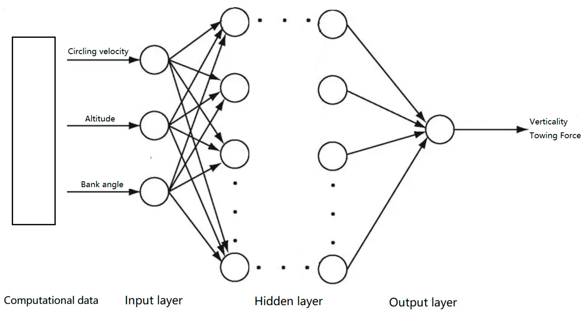
2.2. Neural Network Prediction Methods

2.2.1. Prediction Method Introduction

Neural network algorithms offer an increasingly prominent method for numerical prediction. The BP neural network, a widely adopted multi-layer feed-forward architecture, leverages the error backpropagation algorithm for training. This makes it particularly valuable for prediction tasks in various engineering applications, as evidenced by research in [15,16,17].
The architecture of a neural network prediction model comprises an input layer, one or more hidden layers, and an output layer. The number of neurons in the input layer corresponds directly to the number of features in the data. Similarly, the output layer typically possesses a number of neurons equal to the predicted classes. The hidden layers, of which there can be multiple, offer flexibility in model design. Within this layered structure, neurons exert mutual influence on their respective states. When the output layer generates predictions with significant errors, the neural network will back-propagate according to the error. This involves updating and adjusting the weights and thresholds of different nodes until the predicted output aligns closely with the actual values.
In this paper, the input of the neural network is three-dimensional data consisting of the circling velocity, circling altitude and bank angle of the towed UAV. The outputs consist of the towing force and verticality of the cable during stable circling under these parameters. To enhance accuracy in predicting target data and reduce computational load during training, the approach involves training two separate neural networks: one for predicting cable verticality and another for predicting towing force. Each neural network is designed with two hidden layers, and each layer consists of a specified number of neurons. The simplified structure of the neural networks is illustrated in Figure 5.

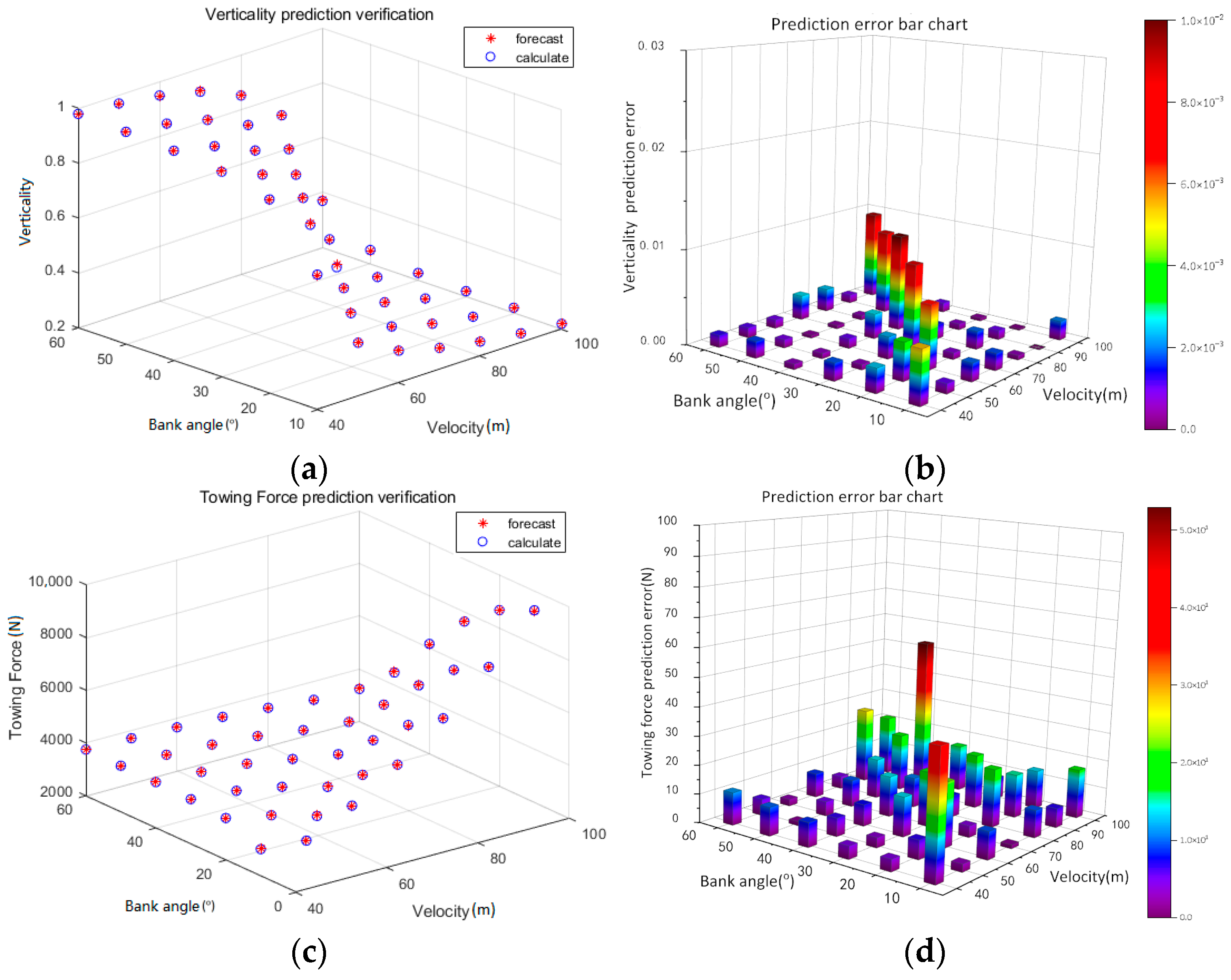
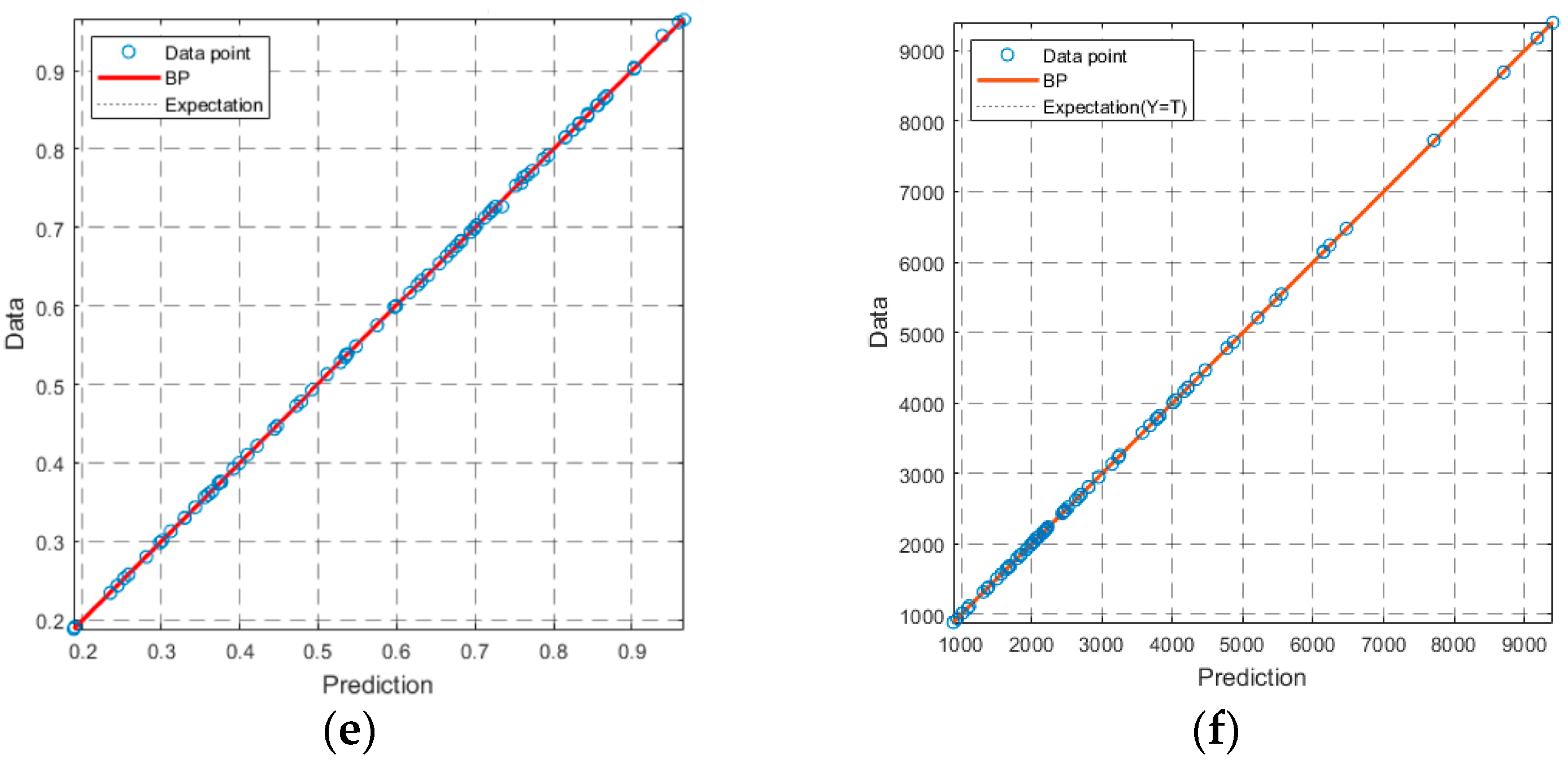
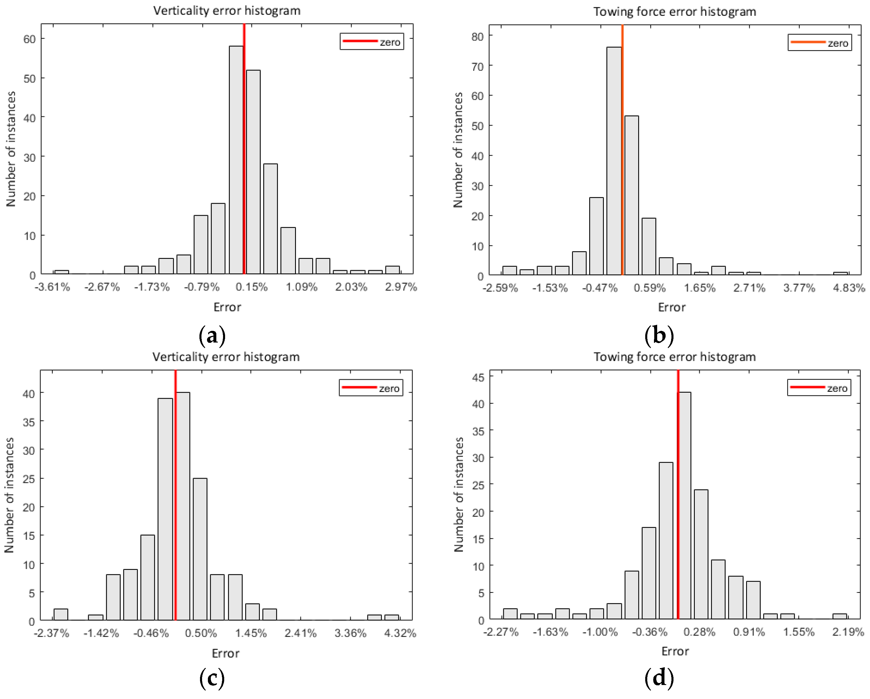
2.2.2. Neural Network Prediction Accuracy Validation

The flight altitude, circling velocity and bank angle of the aircraft are taken as the three-dimensional input variables of the BP neural network, while the other conditions remain constant. The output of the BP neural network is the verticality of the cable and the towing force at the towing point of the cable. Considering the complexity of the mapping relationship between the towing cable and the circling parameters of the carrier aircraft, this paper adopts the double hidden layer BP neural network training method. The basic parameters of the system are as follows Table 3:
The verticality and towing force of the free-end towing cable at a cable length of 4000 m and a flight altitude of 6000 m are chosen for verifying prediction accuracy. Figure 6 shows the accuracy comparison between the predicted value and the actual calculated value. Based on the observation of the verticality scatter plot, it can be observed that for the majority of data points, the predicted results exhibit minor errors compared to the calculated results. However, at the points where there are significant changes in verticality, the errors tend to increase. This is even more evident in Figure 6b where, at a bank angle of 60 degrees and a speed of 100 m/s, a maximum error of around 3% (0.011) is observed. This is likely due to the intricate characteristics of the cable under circling conditions and the significant changes in verticality within the specified area, making it challenging for the neural network to predict accurately. Nonetheless, the neural network exhibits consistently minimal prediction errors, averaging around 0.6% (0.002). In terms of towing force, the largest error is approximately 1% (50 N). Other neural network prediction simulations in more states are presented in the results section; these results suggest the viability of employing a neural network for predicting the state parameters of a cable under uniform circling motion.
In the end free state, it takes about 20–30 s to compute each instance using direct computation; this time is even longer in the end-fixed state, whereas the prediction using the BP neural grid takes less than 1 s, which greatly reduces the computation time despite some errors. This provides the basis for a large number of calculations for the next PSO algorithm.

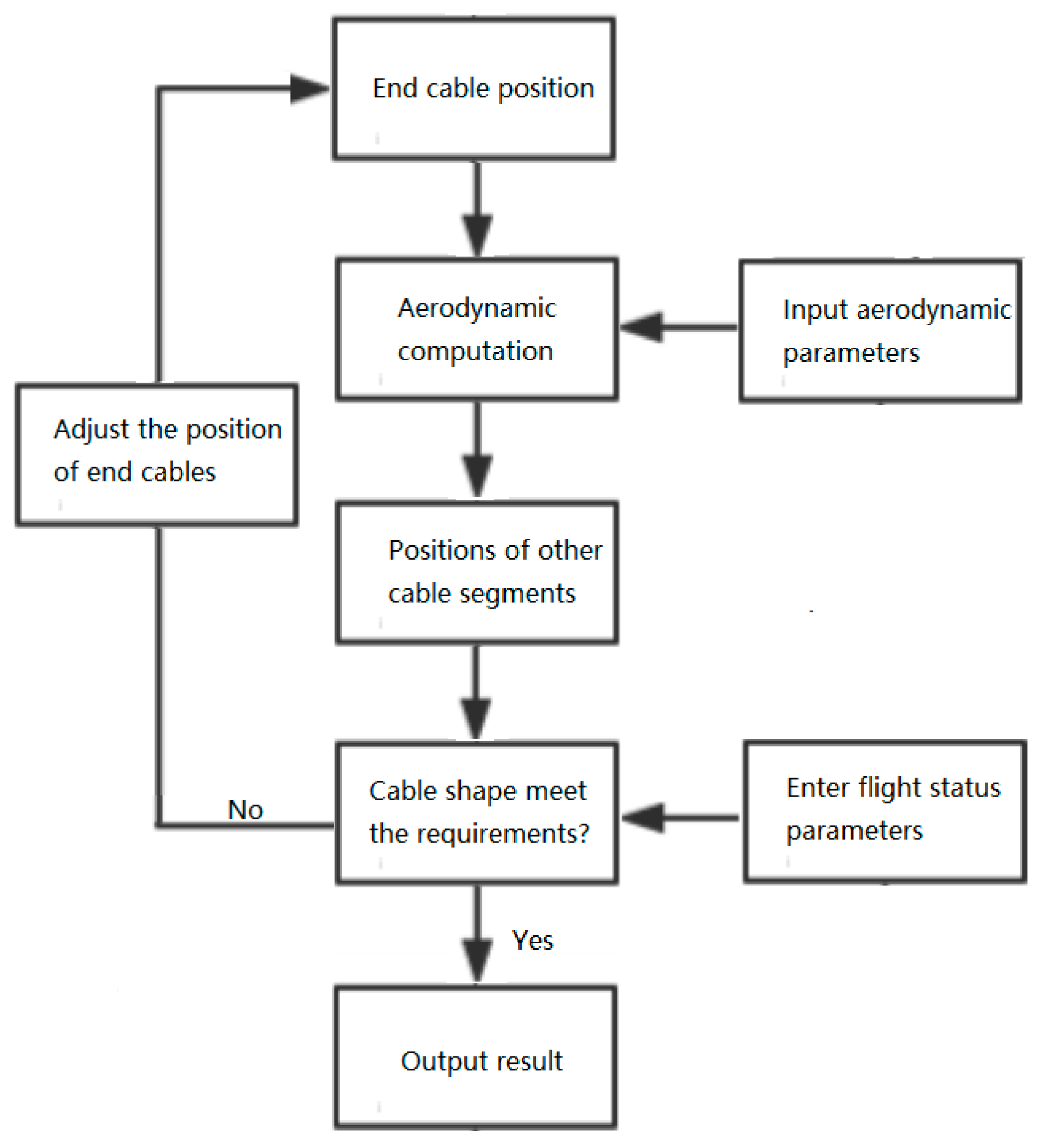
2.3. Optimization Methods

The fitting function obtained through neural network training significantly accelerates the computation time of the towing cable under various circling states. The Particle Swarm Optimization (PSO) algorithm aims to find the optimal solution by simulating the movement of particles within the search domain. PSO’s advantage lies in its simplicity, ease of implementation and requirement for fewer tuning parameters, showcasing excellent global optimization capabilities [18,19].

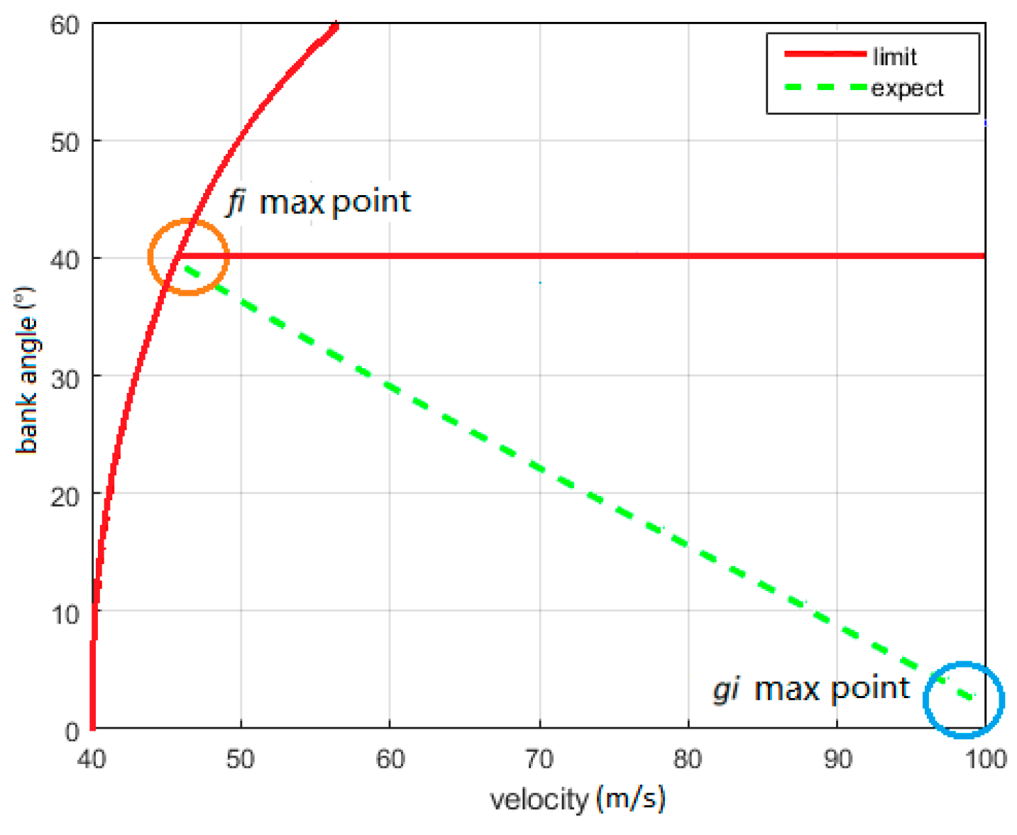
2.3.1. Segmentation of the Search Area

The verticality of the towing cable is essential for its transmission efficiency, with higher verticality associated with enhanced performance. Maintaining a verticality threshold of at least 70% ensures the cable’s proper functionality [11]. While increasing the cable length enhances verticality, it also intensifies towing forces at the connection point with the aircraft, disadvantaging the circling aircraft. Similarly, lowering the aircraft’s speed can boost cable verticality, but excessively slow speeds may lead to stalling, reducing flight efficiency and potentially resulting in adverse consequences. This emphasizes the importance of evaluating towing cable performance by not only examining the cable itself but also considering the aerodynamic efficiency of the circling aircraft. The paper proposes a method that involves partitioning the particle swarm search area into regions to systematically analyze the performance aspects of both the aircraft and the towed cable. This approach aims to optimize the verticality of the towed cable to meet operational requirements while ensuring the satisfactory flight performance of the aircraft. Furthermore, this technique intends to enhance the search efficiency of the PSO algorithm and alleviate the computational burden.
This paper begins with an analysis of the circling performance of the aircraft. During circling maneuvers, the lift generated by the wings changes along the bank angle. As a result, the aircraft experiences a shifted lift component, leading to an increase in the stall boundary. In order to maintain a consistent flight altitude while circling, the velocity necessary for the aircraft’s lift component to balance the aircraft’s gravitational force is termed as the circling velocity. However, the circling velocity typically exceeds the aircraft’s stall speed.
For the selection of stall speed, Table 4 presents flight performance parameters for several common large unmanned aerial vehicles (UAVs). In this study, the Heron TP, developed by Israel Aerospace Corporation (IAC), has been chosen as the designated towed cable carrier. The stall speed of the towed carrier is set at 40 m/s [20,21].
Furthermore, aircraft maneuvering is also limited by the load factor. During level flight, when an aircraft is circling at low speeds, the wings may experience a certain degree of airflow disruption, resulting in buffeting. The buffeting boundary is typically associated with aircraft load factors. To maintain the maximum buffet margin and ensure aircraft maneuverability, an acceptable limit of the load factor has to be determined. Most aircraft usually choose load factor limits that can withstand up to ηmax = 1.3 G load factors, allowing for turns with a bank angle of 40 degrees without encountering buffeting, corresponding to the “1.3 G buffet limit altitude”. The buffet limit altitude for commercial airliners typically exceeds 20,200 feet (6100 m). This paper primarily targets medium to large UAVs, where circling towing altitudes are lower than the typical buffet altitude limit for commercial airliners. Therefore, the calculations limit the search range to circling with the bank angle capped at 40° [22].
In this study, the parameters are set between the circling velocities of 40 m/s (typical stall speed) and 100 m/s, alongside bank angles ranging from 0 to 60 degrees. By considering the velocity and bank angle restrictions discussed earlier, the calculation regions can be divided as shown in Figure 7. The boundaries illustrate limitations due to buffeting and stalling regions.
In addition to the prescribed limits on the velocity and bank angle, it is crucial to address concerns regarding the verticality of the towing cable. A verticality below 60% may lead to excessive cable curvature, consequently diminishing operational effectiveness. It is essential to strategically narrow down the search region by accounting for the verticality constraints. The evaluation of these cables is complex due to the intricate changes in shape.
For the cable trailing at different heights, the shape of the cable exhibits intricate variations. Consequently, verticality numerical constraints are directly integrated into the evaluation function, as expressed in the equation below:
{ F = ( 1 K ) f + K g ( l > 0.6 ) F = σ min ( l i < 0.6 )
where (revisionC1,3)F is the total evaluation function value, and K, f and g are the total weight value, the cable information evaluation value and the position evaluation value, respectively. li is the verticality of the cable and σmin is a constant value to exclude the points where the verticality does not meet the requirements, which is set at 0.1.

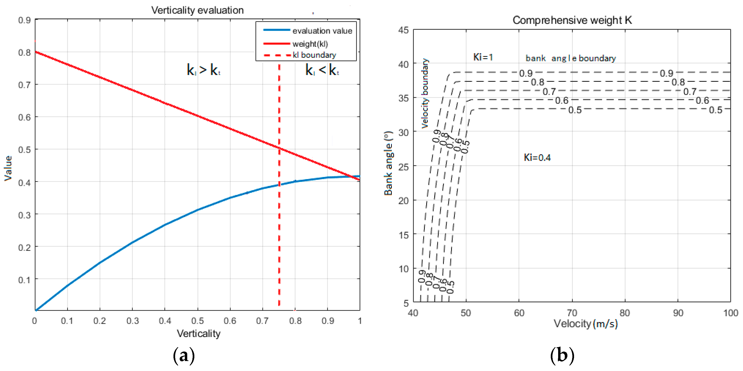
2.3.2. Towed Cable Performance Evaluation Function

There is currently no unified comprehensive evaluation standard for the performance evaluation of trailing cables. Therefore, it is necessary to conduct a weighted evaluation of the existing parameters. Given the characteristics of parameter variations in trailing cables, in order to appropriately balance the verticality and towing force during the aircraft circling process, this paper proposes a method that follows the criteria outlined below:
(1)
Although cable verticality in the search region exceeds 65%, a margin should be allowed due to differing flight conditions. To ensure cable stability, verticality should be prioritized over towing force.
(2)
After the cable verticality reaches a certain degree, a further increase in the verticality has a minimal effect on the cable. At this point, the cable’s lower towing force results in a smaller impact on the aircraft. Therefore, the focus should be on minimizing the towing force exerted by the cable on the aircraft accordingly.
(3)
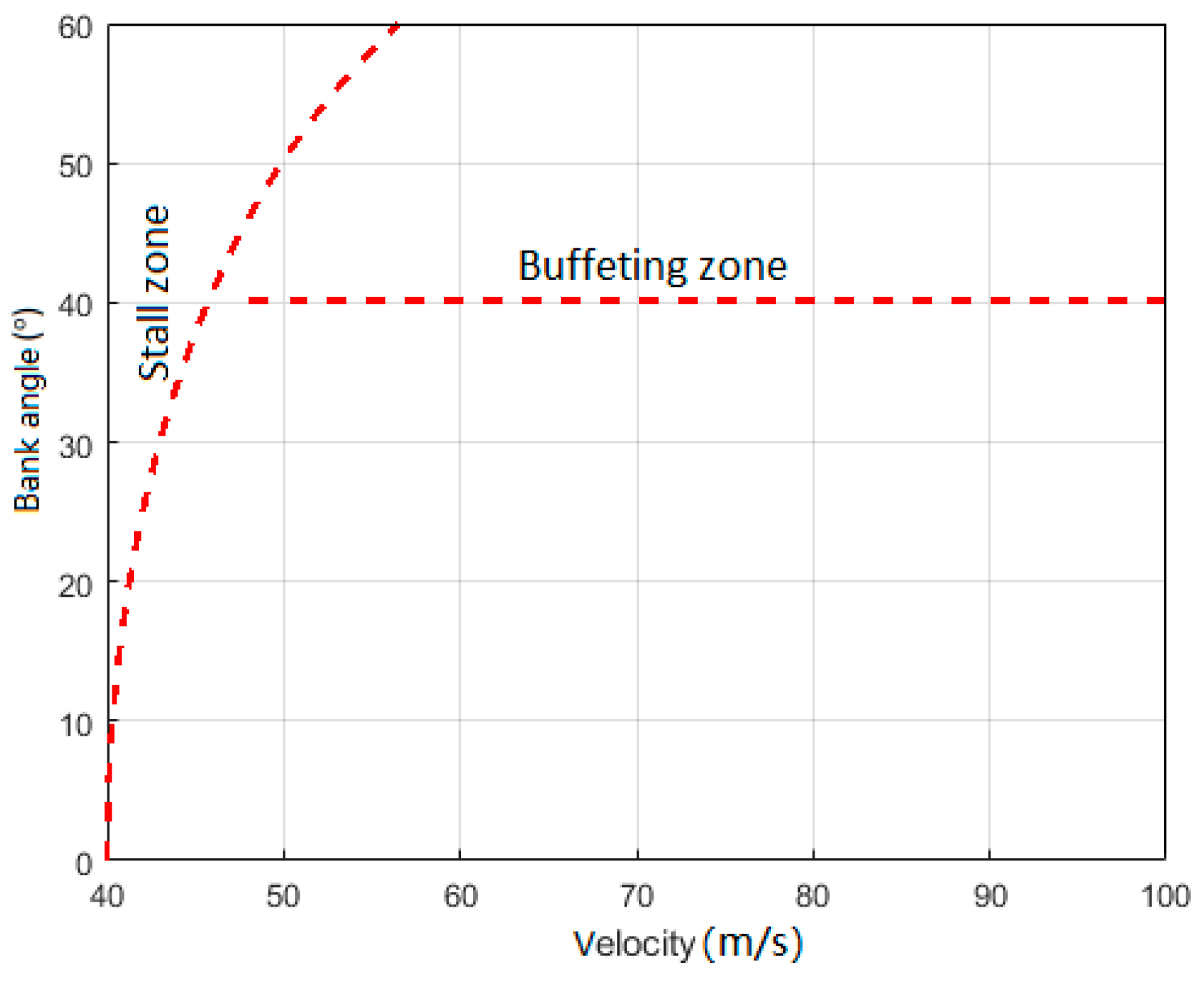
When both verticality and towing force meet specific conditions, it is crucial to maintain a significant buffer from stall and vibration boundaries to enhance the towing aircraft’s aerodynamic performance. This buffer zone ensures that the aircraft operates well within safe aerodynamic limits.
According to the criteria above, a cost function is created. This function incorporates normalized values of the verticality, towing force, bank angle and circling velocity, ensuring all parameters are on a scale of 0 to 1 for better comparison. The normalization formula is as follows:
z i = x i min [ x 1 x n ] max [ x 1 x n ] min [ x 1 x n ]
where zi is the i-th normalized value, and max[xixn] and min[xixn] represent the maximum and minimum values in the dataset.
After normalizing the data, it is necessary to develop an evaluation function to evaluate the performance of the cable and aircraft. First, the evaluation focuses on the aircraft’s performance. This assessment involves evaluating the aircraft’s performance based on the distance between the bank angle and its boundary, as well as the circling velocity and its threshold. Since both the bank angle and speed are crucial for the aircraft’s normal flight, they are each allocated equal weights of 0.5 in the evaluation function for the aircraft, as shown below:
g i = 0.5 × Δ v i + 0.5 × Δ γ i
where gi is the performance evaluation parameter and Δvi and Δγi indicate the normalized distance from the circling velocity and bank angle to their respective boundary limits.
In the evaluation of the cable’s performance, the verticality and towing force are taken into account. The objective of this is to reduce the towing force while adhering to the verticality requirements. This involves assigning dynamic weights to both towing force and verticality. Below are the evaluation factors for the trailing cable:
{ f i = t i k i t + l i k i l k i t = 1 k i l t i = max [ t 1 t n ] t i max [ t 1 t n ] min [ t 1 t n ] l i = max [ l 1 l n ] l i max [ l 1 l n ] min [ l 1 l n ]
where ti represents the difference between the normalized towing force and its maximum value, while li represents the normalized verticality of the cable. k i t and k i l denote the weight coefficients for towing force and verticality, respectively. This ensures that the sum of the weight coefficients for the cable evaluation factors equals 1. To adjust the weight properly, it is crucial to assign a higher value when verticality is low or vice versa. When verticality reaches a specific level, the weight for verticality gradually decreases while the weight for towing force increases. It is important to maintain high verticality and low towing force to enhance cable transmission efficiency while minimizing the loads on the aircraft. In this paper, the weight and evaluation values are linked in a product relationship. Therefore, it is crucial to avoid excessively small weights. Otherwise, an increase in verticality may lead to a reduction in its evaluation value due to an excessively small weight. It is established that cables operate effectively when their verticality exceeds 0.75. Therefore, when the cable’s verticality reaches this threshold, the weight of the towing force equals the weight of the verticality. As verticality increases beyond 0.75, the weight gradually decreases. The maximum verticality considered for the weight is capped at 0.8. The verticality weight is expressed as follows:
k i l = 4 5 2 5 L
where L is the actual value of the verticality of the trailing cable.
The comparison between the evaluated verticality value l i × k i l and the actual verticality value is illustrated in Figure 8a below:
It can be observed that initially the weight of verticality surpasses that of the towing force. When the verticality reaches 0.75, both the weights of verticality and towing force equate to 0.5. Upon surpassing a verticality value of 0.75, although further increases in verticality will still enhance the overall evaluation value of the verticality, the rate of change at this stage is lower compared to the evaluation value, resulting from the reduction in towing force. In essence, the verticality shows a lower sensitivity compared to the towing force.
Considering both the aircraft circling performance and the shape of the cable, the comprehensive evaluation function can be expressed as follows:
F i = ( 1 K i ) f i + K i g i
where Fi is the value of the total evaluation function for the i-th particle, gi and fi are the values of the aircraft performance evaluation parameter and cable’s evaluation parameter, respectively, and Ki represents the total weight used to evaluate the aircraft performance and cable structure.
The range of values for the comprehensive weight, Ki, is depicted in Figure 8b. This figure shows that by extending the boundaries of the circling velocity and bank angle selection inward to 0.8 times their own values, the region for the comprehensive weight Ki is established, which linearly changes. Moreover, at the upper limit of 1 on the boundary, the aircraft’s circling performance exclusively dictates the evaluation function, prompting search points to move away from the boundaries. To accurately reflect the variations in the cable at different altitudes, a lower limit Ki min = 0.4 is selected through trial and error. At this point, the evaluation function is predominantly influenced by the cable’s shape, while also ensuring it stays away from the boundaries. In scenarios where the cable length changes with altitude, subsequent discussions will explore various minimum comprehensive weight factors, Ki min, to identify the most suitable circling parameters for the aircraft.
As operational conditions approach boundaries, the weighting for aircraft circling performance increases rapidly, guiding the optimal evaluation position away from these limits. Ensuring a safe distance from these boundaries subsequently emphasizes favorable cable spatial structures over aircraft-circling parameters in the overall evaluation. Hence, the total weightage of the evaluation value function is expressed as follows:
( 1 K i ) ( 0.5 + 0.5 ) + K i ( k i l + k i t ) = 1
As depicted in Figure 9, at the circling velocity boundary, a decrease in circling velocity results in an increase in bank angle, cable verticality and a reduction in towing force. Notably, an optimal point for the maximum cable performance parameter (fi max) is observed on this boundary(orange circles). Conversely, as circling velocity increases, bank angle decreases, thereby enhancing aircraft flight performance. This optimal point for maximum aircraft performance (gi max) is situated below the computational domain(blue circles).
Thus, achieving a balance between circling velocity and bank angle is imperative. Figure 9 shows that relying solely on the distance between search points and boundaries for assessment may lead to scenarios where the circling velocity diminishes significantly or the bank angle increases significantly. Despite these challenges, the evaluation function value for the carrier’s performance remains high.
To ensure that both the circling velocity and bank angle are kept significantly away from their boundary limits and to avoid scenarios where either velocity is extremely low or the bank angle is excessively high, search particles should aim to approach the desired region (represented by the dashed line in Figure 9). For this purpose, the following formula is proposed to assess the consistency in the relative distances of search points from the circling velocity and bank angle boundaries, thereby introducing the integrated performance index (ni) for the aircraft:
n i = ( 1 Δ x i Δ y i ) 2 + 1
where Δxi and Δγi represent the normalized distances from the velocity and bank angle boundaries, respectively.
The integrated performance index (ni) is utilized to assess whether the changes in the velocity and bank angle at the search point are uniform. When the evaluation values of the velocity and bank angle are equal, indicating the integrated performance index ni = 1, the point is closest to the desired region represented by the dashed line in Figure 9. However, if there is a notable difference between the evaluation values of circling velocity and bank angle, the aircraft may be positioned at an extreme position, resulting in an integrated performance index greater than 1. Although the performance evaluation values might be equal, the integration of the aircraft performance index (ni) acts as a divisor in the total evaluation function, consequently reducing the overall evaluation value. This method ensures that search points are as close as possible to the desired search region. At this stage, the comprehensive evaluation function of the towing cable under uniform circling can be expressed as follows:
F = ( 1 K i ) ( t i k i t + l i k i l ) + K i ( 0.5 Δ v i + 0.5 Δ γ i ) n i
In the subsequent calculations, the calculations for the free-end cable employ the constant lower limit of the comprehensive weight factor Ki min value, as previously described. For calculations under fixed-end conditions, various Ki min values are experimented with for comparison, ultimately integrating considerations of the optimal point position.
Finally, the evaluation method mentioned above is compared with two commonly used methods in current performance evaluation: the Analytic Hierarchy Process (AHP) and the Entropy Weight Method (EWM). Both the AHP and EWM are criteria weighting methods; the difference is that the AHP is a subjective empowerment method, while the EWM is an objective empowerment method that calculates weights based on the amount of information (entropy) contained in each criterion. The weights of each parameter of the two methods are calculated as follows Table 5.
For the verification process, an altitude of 6000 m and a cable length of 4000 m were selected. The parameters range from a speed of 35 to 100 m/s and a bank angle of 5 to 60 degrees. The Figure 10 below illustrates the results obtained from different evaluation methods.
The values of the optimal point under different evaluation methods are shown in the table above, Table 6. It can be seen that the weights in the EWM are determined based on the fluctuation of different parameters. As a result, the EWM assigns the highest weight to the towing force, leading to the lowest towing-force evaluation result among the three methods. Moreover, the results from the EWM showed that the circling velocity of the carrier is only 35 m/s, which is dangerously close to the stall boundary. Under such conditions, towing the cable is undoubtedly risky. On the other hand, the AHP yields the best verticality result as shown in the table, which aligns with the significant impact of cable verticality on its operational state. However, the towing force exceeds 3600 N. Additionally, when the cable’s verticality exceeds 75%, it can maintain normal operation without the need for additional towing force, although the method proposed in this paper does not outperform the EWM in towing force or the AHP in verticality. However, it achieves a balance between these aspects, ensuring the towing carrier does not stall while maintaining the performance of the cable

3. Calculation Results

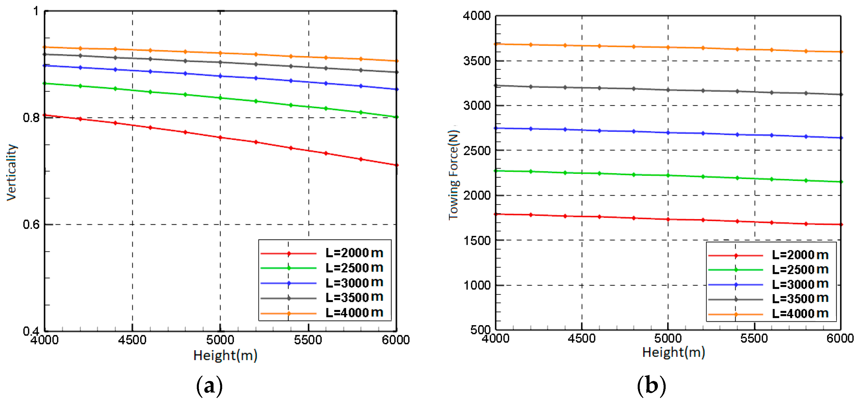
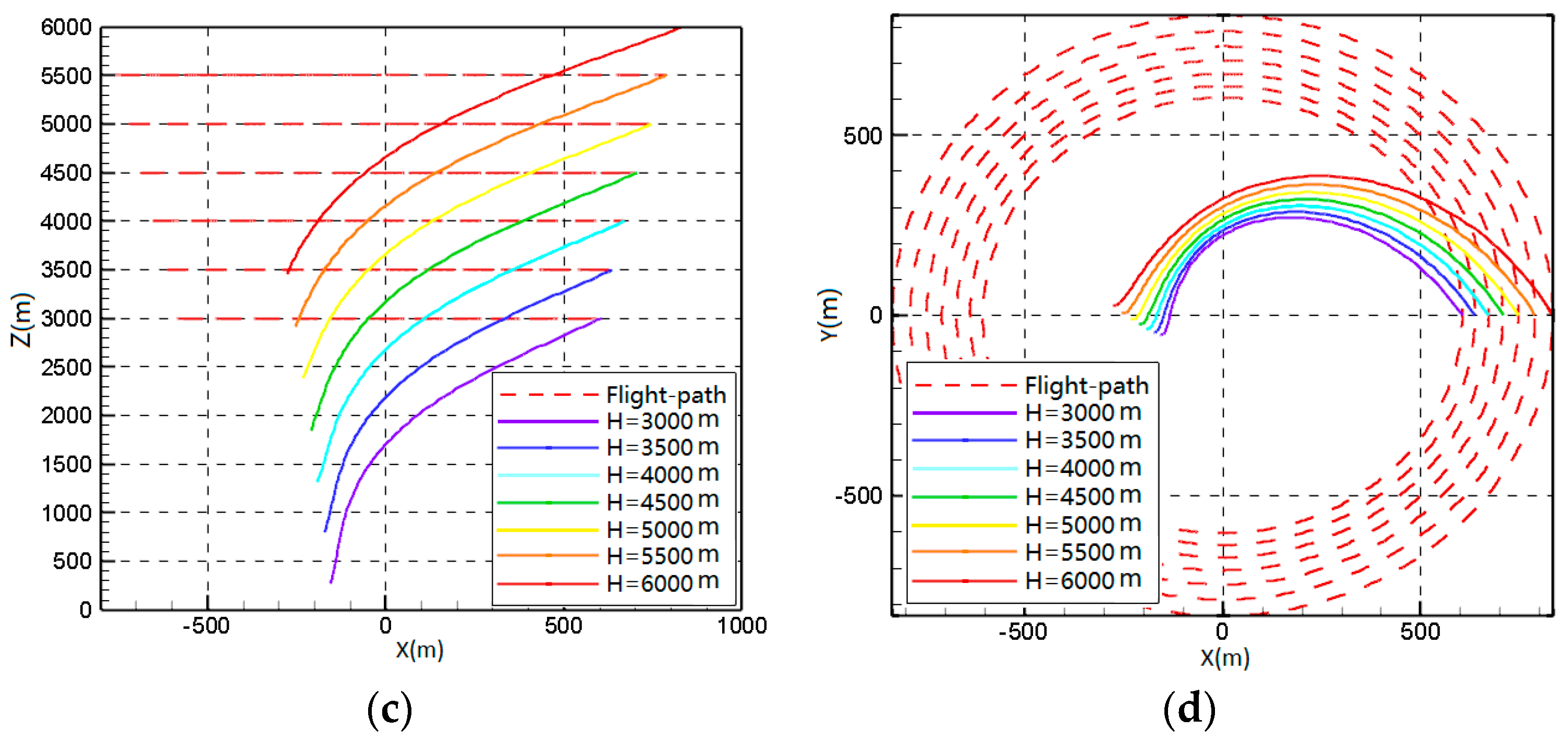
3.1. Different Circling Altitudes

3.1.1. End-Free State CABLE

For the towing cable in a free-end state, this paper examines the circling conditions at a constant altitude with varying cable lengths, bank angles and velocities. To proceed with the calculations, it is essential to determine the predetermined altitude in advance.
In this study, a trained BP neural network is employed to predict the parameters of the towing cable at various altitudes using an aircraft circling at a velocity of 40 m/s with a bank angle of 20 degrees, as depicted in Figure 11a,b. The results indicate that the predicted trends align well with the existing literature [11], demonstrating that an increase in circling altitude leads to a decrease in the verticality of the cable, regardless of its length. Specifically, as the circling altitude rises, the verticality of cables of different lengths diminishes, with shorter cables experiencing a more pronounced rate of reduction.
For a free-end towed cable with a constant length of 3000 m, simulations were conducted at various circling altitudes, as depicted in Figure 11c,d. It is important to note that in this study, the circling velocity is the indicated airspeed (IAS). As the IAS remains constant, the true airspeed (TAS) increases with altitude due to decreasing air density. Consequently, the circling radius expands with altitude, altering the cable’s spatial structure. Considering this variation in cable behavior at different altitudes, altitudes of 2000 m and 6000 m were selected as optimal circling altitudes for search optimization.

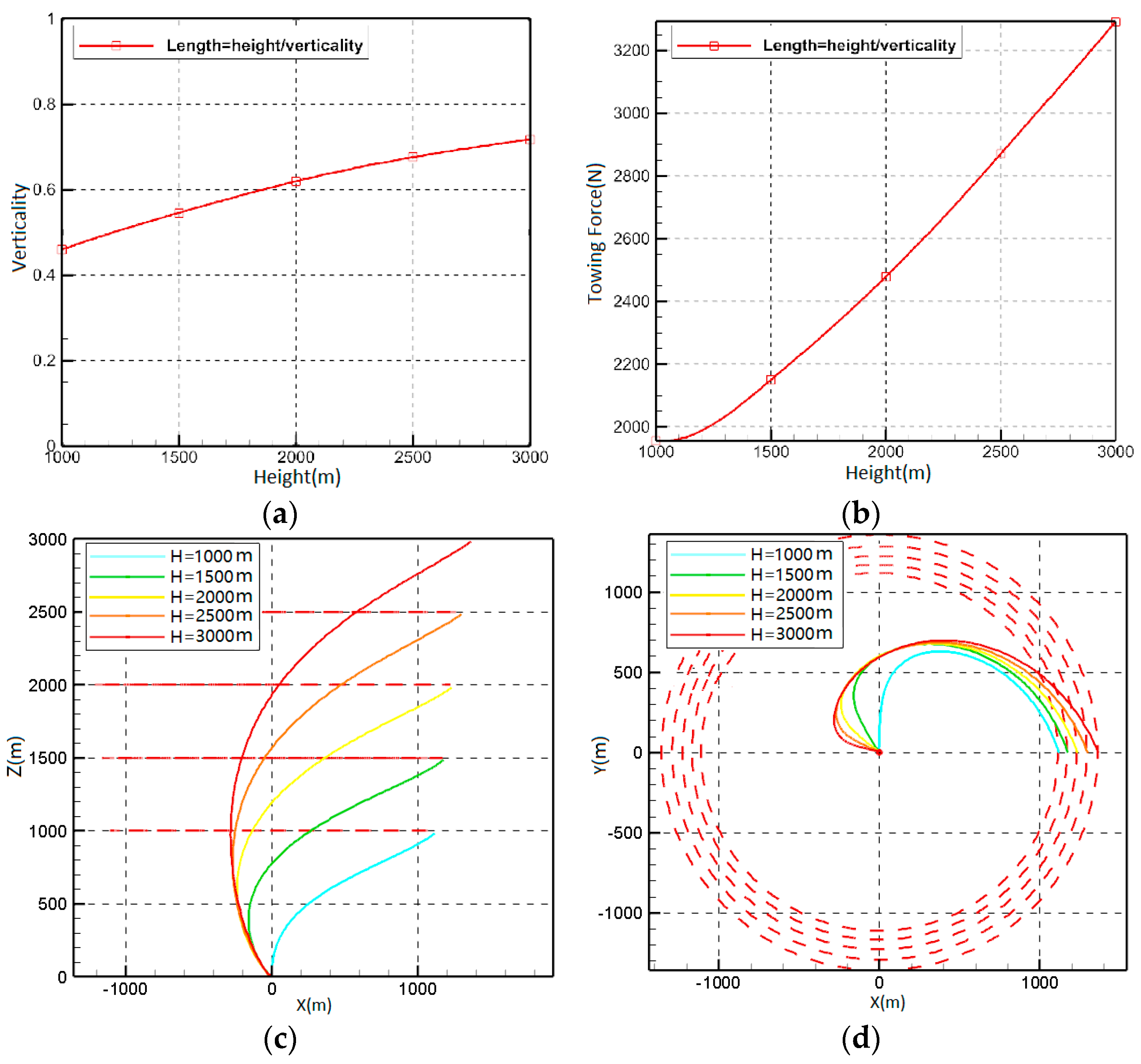
3.1.2. Fixed-End State Cable

For UAVs or other aircraft requiring aerial recharging, the towed cable remains fixed at the end, typically to a ground station, with its length increasing as the aircraft ascends in circling altitude. Hence, the selection of a specific altitude position becomes unnecessary and only predictions of the cable’s parameters and shape are carried out. When the end of the cable is fixed to the ground, the towing force increases rapidly with rising flight altitude. By an altitude of 3000 m, the towing force is nearly as high as that observed when the end is free at 4000 m, as shown in Figure 12b.
Considering that excessively long towed cables can generate significant reaction forces at the cable’s end, potentially exceeding the structural capacity of the underlying power supply, this study selects a flight altitude range of 500 m to 3000 m for the towed cable under fixed-end conditions [23]. The cable state under different altitudes is calculated, as illustrated in Figure 12a,b.
Since the cable’s end is fixed to the ground, the circling altitude divided by the verticality equals the cable’s length. The below Table 7 summarizes the cable length at different circling altitudes.
Figure 12c,d illustrate the shape of a fixed-end cable towing at different altitudes, demonstrating that the cable length varies with the flight altitude of the aircraft. As the cable length increases, the verticality of the cable also increases, but the rate of its increase gradually becomes slower. Regarding the towing force, similar to the trend in the end-free state, the cable towing force gradually increases as the flight altitude of the carrier aircraft increases and the length of the cable increases.

3.2. Neural Network Training

To facilitate neural network training, this study establishes an end-free state cable by employing a multi-body dynamics model. This model calculates and simulates various scenarios involving different cable lengths, circling velocities and bank angles at altitudes of 2000 m and 6000 m. Step sizes are set at 5 m/s for circling velocity, 100 m for cable length and 5° for bank angle.
Figure 13 shows the regression analysis of neural network grid training, showing predicted values against actual calculated values. The ideal regression curves for different parameters are indicated by diagonal lines, with blue scatter points representing actual testing results. An alignment with the red diagonal line indicates agreement between predicted and calculated values. The results indicate a strong agreement between towing force and calculated values for various towing cable conditions. Scatter points closely follow the regression curve, signifying high accuracy. However, verticality prediction is slightly lower due to complex mapping with circling state parameters, though deviations from the regression curve are minimal.
For stable circling towing cables at altitudes of 2000 m and 6000 m, the BP neural network data for stable circling towing cables at altitudes of 2000 m and 6000 m were compared in terms of verticality and towing force errors using the Latin hypercube sampling (LHS) method. This method involves selecting random sampling intervals of 10 for the circling velocity and bank angle and intervals of 500 and 1000 for altitudes at 2000 m and 6000 m, respectively.
The error distribution of these sample points is shown in Figure 14 and Table 8. The overall error between the predicted values and the actual calculated values is relatively small. The maximum errors in towing force are 97.07 N and 34.62 N, while the maximum errors in verticality are 0.0084 and 0.0053. Although the sample size for the test is limited, and the relative error across the actual overall calculation range may be larger, the BP neural network predictions effectively reflect the parameter variation trends in the actual towing cables. Therefore, using these predicted values for further optimization is feasible.
This study extends its analysis by employing a trained BP neural network to offer a comprehensive preliminary prediction within the forecasted range. Figure 15 depicts contour plots illustrating the variations in cable verticality and towing force along the circling velocity and bank angle for different cable lengths. It can be seen that the prediction results are consistent with the calculations in the previous section: as the circling velocity increases and the bank angle decreases, the cable’s verticality gradually decreases and the towing force increases. As the circling velocity decreases and the bank angle increases, the verticality gradually increases and the towing force gradually decreases. The length of the cable is positively correlated with the cable’s verticality and negatively correlated with the towing force. The longer the cable length, the better the cable’s verticality at the same circling velocity and bank angle.
In terms of altitude, as altitude decreases, the cable verticality under the same circling parameters also improves. The contour plot of cable verticality for an altitude of 2000 m with a cable length of 2000 m is similar to the cable verticality for a 3000 m cable length at an altitude of 6000 m.
Similarly, in terms of towing force and the circling radius at the cable end, the numerical values are smaller at a 2000 m altitude. This is likely due to the fact that when the aircraft speed is constant, the density increases as altitude decreases. Consequently, the true speed of the aircraft decreases with decreasing circling altitude, resulting in a decrease in the circling radius of each part of the antenna. It is worth noting that at a 2000 m altitude when the cable length is too short (l < 500 m), the variations in verticality and towing force become less apparent. This may be attributed to the increased proportion of aerodynamic forces on the cable caused by the excessively short cable length.
Figure 16 depicts contour plots illustrating the variations in cable verticality and towing force along with the circling velocity and bank angle under fixed-end conditions. The trend in verticality is similar to that of the free-end condition, with the cable’s verticality gradually increasing as circling velocity decreases and the bank angle increases. However, in the fixed-end condition, the verticality changes uniformly with the circling parameters, without distinct transitions.
Figure 16b shows that when the circling velocity is low and the bank angle is steep, the contour plots shift to warmer colors as the altitude increases, indicating a rise in towing force with flight altitude. This observation matches previous calculations. Notably, under fixed-end conditions, particularly at lower flight altitudes with shorter cable lengths and higher circling velocities, the towing force experiences a significant surge, exceeding the towing forces observed in other circling states by a substantial margin. Additionally, unlike the free-end condition, the towing force under fixed-end conditions increases as cable length decreases. This surge likely occurs because the cable is fixed to the ground, generating a substantial reaction force to restrict the cable’s end position when the cable is short and the circling velocity is high. Since the aerodynamic force generated by the cable is relatively low in this scenario, the reaction force is largely transferred to the towing point, increasing the force at this point. Therefore, when the cable end is fixed to the ground, the towing aircraft should maintain a consistent flight altitude and reduce circling speed to minimize towing force.
To conduct sensitivity analyses of the cable’s behavior under various circling parameters, this study selects an initial position near the center for each solution space and adjusts the values accordingly. The below Table 9 summarizes the effects of changes in the flight altitude, circling velocity and bank angle on the behavior of the trailing cable system.
In the analysis under the free-end condition, it is evident that circling velocity exerts the most significant influence on both the verticality of the cable and the towing force. Conversely, the length of the cable has the least impact on these factors, regardless of whether the altitude is 2000 m or 6000 m. Under the fixed-end condition, changes in the bank angle prove to be the most sensitive factor affecting the verticality of the towing cable and the towing force.

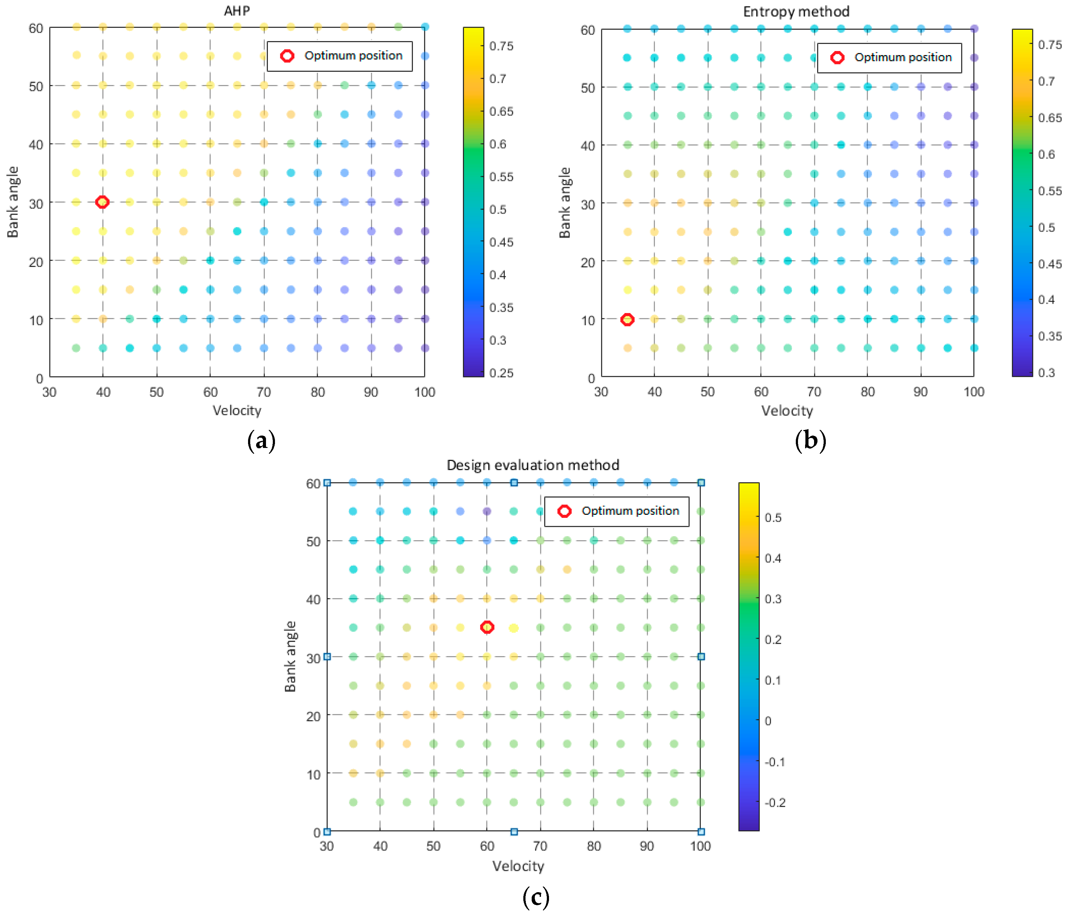
3.3. PSO Search Results

3.3.1. PSO Search Results for End-Free Condition

In this study, PSO search will be employed to determine the optimal values. Initially, the constraint region, as outlined in the previous section, will be defined. Within this region, the positions of 100 particles will be initialized. As mentioned earlier, the aircraft’s flight altitude is fixed within this region, the while bank angle and velocity have predefined ranges.
The cable parameters primarily depend on the length of the cable deployed by the aircraft. Longer cable lengths result in higher cable verticality, but they also lead to increased towing force due to the added cable mass. Consequently, the main objective of the PSO algorithm is to find the optimal cable deployment length while adhering to the constraints. Specifically, the aim is to minimize towing force while maximizing cable verticality.
The PSO algorithm initiates with 100 particles and defines the search range as follows: cable length from 0 to 6000 m, circling velocity from 40 to 80 m/s and bank angle from 10 to 40 degrees. The maximum speed in each direction typically ranges between 10% and 20% of the search range; in this paper, it is set to 10%. The particle position and velocity are updated according to the equations shown below:
{ v i = ω v i + c 1 r a n d ( p b e s t x i ) + c 2 r a n d ( g b e s t x i ) x i = x i + v i
where xi and vi are the position and velocity of individual particles, respectively. ω is the inertia weight factor which is set to 0.8 after testing so that the algorithm can ensure the stability of the results while at the same time maintaining the highest computational efficiency. c1 and c2 are the self-learning factor and the group learning factor, respectively, both set to 0.5.
In this study, a circling altitude of 2000 m was utilized to assess the stability of the PSO algorithm. The results from multiple search iterations are presented in Table 10 below:
It can be seen that after the number of iterations reaches 100, the search results no longer change. In order to ensure the convergence of the results, the next search iteration number in this paper is set to 120.
To achieve this, a total weighting factor, Ki min, is used, set to 0.4. This factor is crucial for balancing aircraft performance with cable structure. The resulting comprehensive evaluation function and structural characteristics for towing the cable are summarized in the table below Table 11.
It can be observed that, compared to an altitude of 6000 m, the optimal position of the search point at an altitude of 2000 m results in a smaller towing force on the cable and better cable verticality. This finding aligns with earlier predictions. Additionally, the lower altitude and increased air density improve the aircraft’s aerodynamic performance. This improvement allows the circling aircraft to approach the constraint boundaries more closely, achieving a better cable shape. Therefore, if other conditions are met, the circling aircraft should aim to lower the circling altitude as much as possible during the towing process. The simulation calculations of the circling parameters based on the final PSO results illustrate the shape of the towing cable, as shown in Figure 17.

3.3.2. PSO Search Results for Fixed-End Condition

To enhance the endurance of large drones, it is necessary for drones to connect to ground-based facilities via a towing cable for aerial recharging. This paper focuses on optimizing the stable circling trajectory parameters during aerial recharging using the PSO search algorithm.
As previously mentioned, the length of the towing cable under fixed-end conditions is related to the flight altitude of the aircraft, making the variation in performance parameters complex. Therefore, the method of directly setting the total weighting factor Ki min as a constant (Ki min = 0.4) is no longer applicable. In this section, different values of the total weighting factor Ki min are chosen for the search process to compare and evaluate the comprehensive optimal point. The total weighting factor reflects the trade-off between the aircraft’s performance and the cable’s performance parameters in the overall evaluation function. A Ki min value that is excessively small tends to shift the search process towards the predefined boundaries set by the aircraft’s performance limits. Conversely, an excessively large Ki min value leads to the formation of a cable shape that fails to meet the operating requirements. The results from the trial-and-error selection of various Ki min values are presented below Table 12.
It can be observed that the total weighting factor Ki min is closely related to the search for the optimal solution. As Ki min gradually increases, the optimal solution moves further away from the boundaries defined via circling velocity and bank angle limitations. However, its cable verticality and towing force gradually decrease. Conversely, when the Ki min decreases, the optimal solution approaches the boundaries, while the performance of the cable gradually improves. A comparison of the optimal solutions for different Ki min values is illustrated in the following Figure.
In Figure 18a, a Ki min value of 0.2 achieves a cable verticality of 86%. However, with an aircraft circling velocity of 52.2 m/s and a bank angle of 32 degrees, this circling state nearly approaches the boundary of buffeting. Furthermore, the reduced circling velocity raises concerns about the aircraft’s ability to provide sufficient lift during circling.
When the Ki min value is increased to 0.35, the flight is maintained at an altitude of 3000 m. Both the circling velocity and bank angle of the aircraft move further away from the boundaries. Nevertheless, the cable’s verticality decreases to around 76%. Although the cable remains operable in this configuration, the increased curvature may weaken the operational efficiency.
Considering these aspects, the optimal stable circling parameters for the fixed-end state of the towing cable are determined using a Ki min value of 0.25. Here, the optimal point significantly distances itself from the boundaries, ensuring that both the cable verticality and towing force are sufficient to meet operational demands. The shape of the cable in this state is depicted in Figure 19.

4. Conclusions

To address the issue of optimizing the configurations of a cable in a steady-circling state, this study proposes using a BP neural network model to predict the state parameters of the towing cable, significantly reducing the computation cost. The results indicate that the BP neural network effectively reproduces the mapping relationship between the circling state of the orbiting aircraft and the parameters of the cable, with minimal error between the predicted results and the simulated calculations. The predicted results show the following:
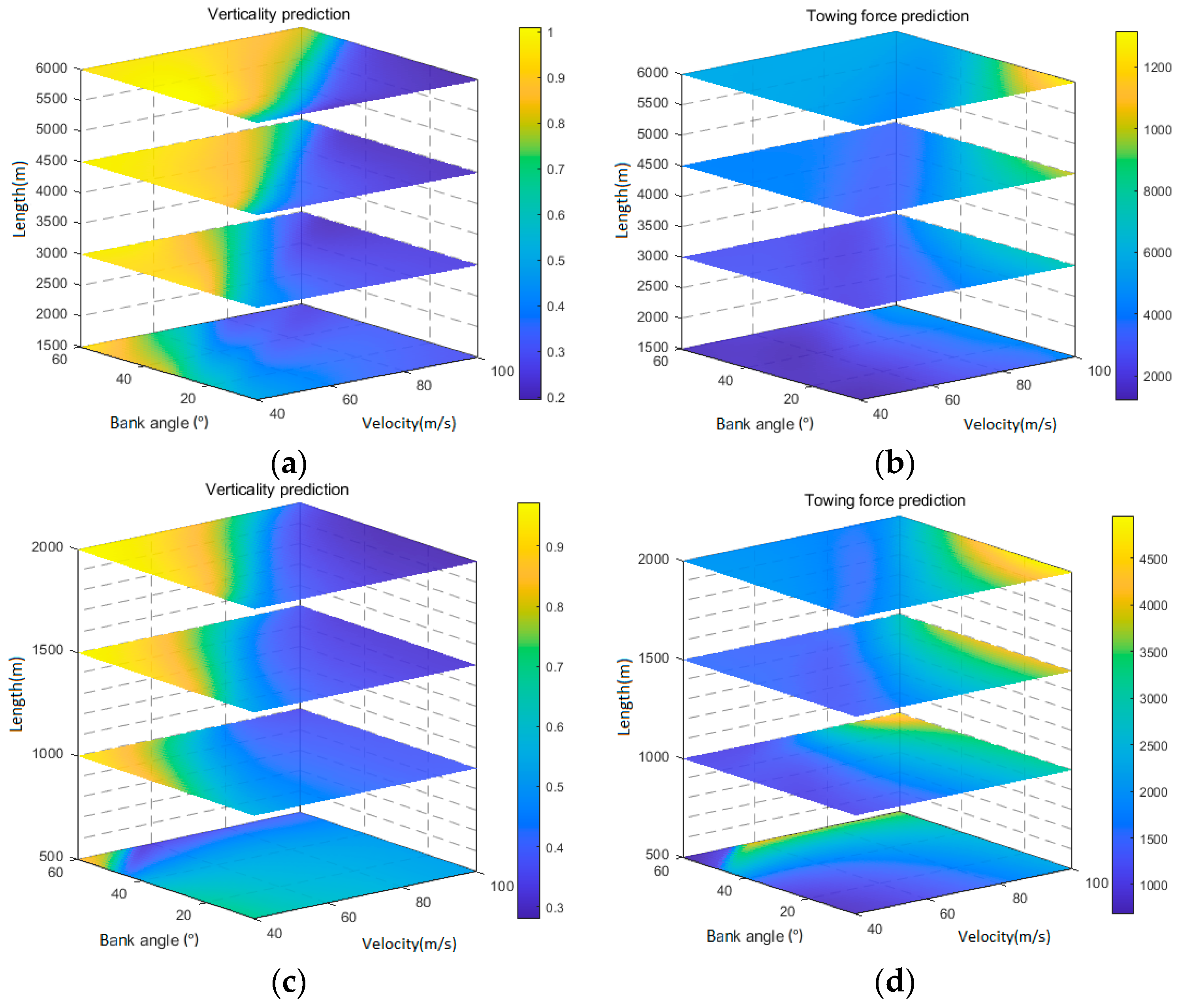
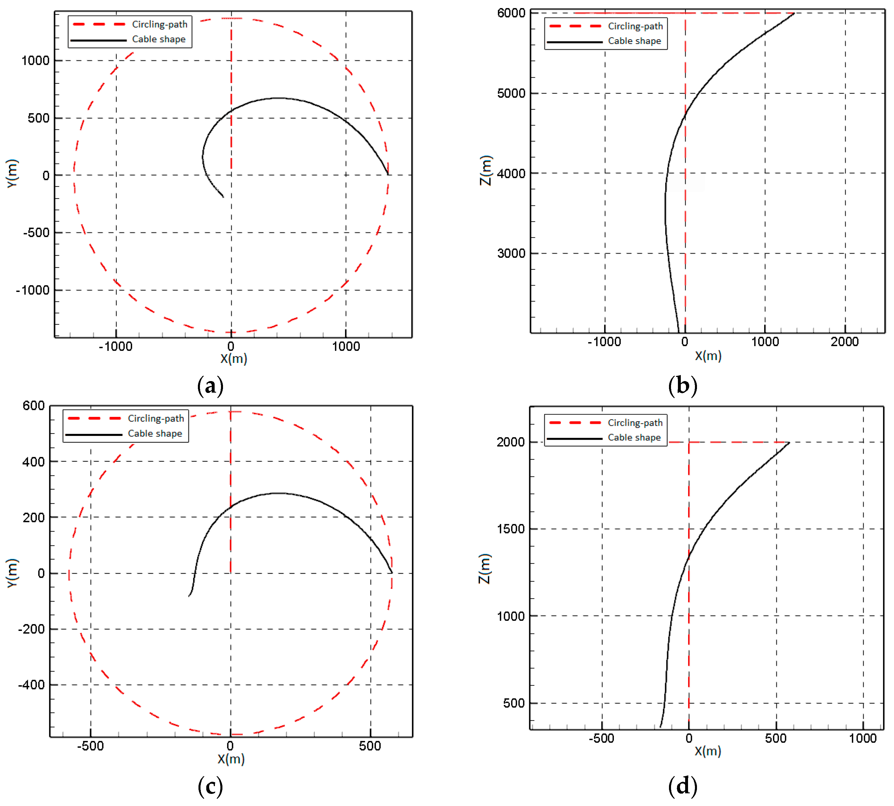
  • Under free-end conditions, the shape of the towing cable progressively enhances with an increase in the bank angle of the aircraft coupled with a decrease in circling velocity. Moreover, increasing the length of the cable within the same circling condition results in better vertical alignment, although it also results in an increase in towing force, requiring consideration and the balancing of the trade-off between vertical alignment and towing force. Within the range of 2000 m to 6000 m, lowering the altitude further improves the cable’s shape under identical circling conditions. Moreover, a reduced altitude enhances the aerodynamic efficiency of the aircraft. Consequently, it is advisable to minimize circling altitude whenever feasible.
  • Under fixed-end conditions, the transition of the cable’s verticality changes gradually, similar to the trend observed in free-end scenarios. However, the towing force exhibits more drastic changes when the cable is fixed at the end. Under this setup, the orbiting aircraft must carefully maintain a specific circling altitude and cable length while ensuring that the circling velocity remains within acceptable limits. Otherwise, a rapid increase in towing force may occur, demanding greater attention to the material properties and structural integrity of the aircraft.
Additionally, this paper introduces a comprehensive evaluation function to assess the circling performance of the towing cable. The evaluation function considers both the cable’s shape and the aerodynamic efficiency of the orbiting aircraft. The function aims to optimize the cable’s verticality and towing force while preserving the aircraft’s aerodynamic performance. Additionally, it aims to minimize the cable’s impact on the orbiting aircraft, thereby meeting operational requirements.
Moreover, this study employs the PSO algorithm to address the challenges of airborne communication transmission and aerial recharging for UAVs. The algorithm optimizes the stable circling parameters of the cable under both free-end and fixed-end conditions, resulting in the following results:
  • Under free-end conditions at an altitude of 6000 m, the evaluation function reaches its optimal state with a cable length of 5258 m, a circling velocity of 62 m/s and a bank angle of 28°, where the cable verticality is 79% and the towing force is 4400 N.
  • Under free-end conditions at an altitude of 2000 m, the evaluation function reaches its optimal condition when the cable length is 2052 m, the circling velocity of the orbiting aircraft is 55 m/s and the bank angle is 33°. At this point, the cable verticality is 81% and the towing force is 1800 N.
  • Under fixed-end conditions, the evaluation function reaches the optimal state when the circling altitude is 2470 m. Here, the cable extends over 3758 m, with the orbiting aircraft maintaining a consistent circling velocity of 55 m/s, accompanied by a bank angle of 29°. This setup results in a cable verticality of 84%, demanding a towing force of 2546 N.
Under ideal windless conditions, for medium-sized UAVs, flying according to the circling parameters mentioned above after cable deployment can ensure both the stability of the aircraft and the absence of vibration phenomena while meeting the requirements for cable verticality and towing force. For other types of aircraft, the method outlined in this paper can be used to modify the boundaries of the flight performance and search for the optimal point, providing guidance and reference for various aerial tasks requiring the use of towing cables, such as aerial recharging and relay communication transmission.
This paper effectively identifies the optimal circling parameters for towing cables under specific conditions using modeling and predictive methods. However, the study primarily focuses on low-speed flight and medium-sized UAVs, thus restricting the scope of calculation and prediction. To enhance its applicability, there is still room for improvement in the application of the evaluation functions and search methods. Moreover, some assumptions are made in this paper to simplify the calculation, which sacrifices the accuracy to a certain extent; at the same time, environmental factors such as wind need to be taken into account in the actual engineering application. In practical engineering applications, environmental factors such as wind must be taken into consideration. Therefore, the results presented here are specifically applicable under ideal windless conditions and adjustments may be necessary for real-world applications. It is important to note that the primary motivation of this study is to swiftly predict the impacts of circling velocity, bank angle and flight altitude on the cable’s shape. This capability accelerates the identification of cable behavior without the need for time-consuming simulations.
In future studies, researchers could integrate the prediction of stable circling cable states with autonomous control and other relevant technologies. This integration holds great potential, particularly in fields such as relay communication transmission and UAV aerial recharging. This integration would better meet the needs of missions with medium- and large-sized UAVs.

Author Contributions

Software, L.F.; Formal analysis, Z.F.N.; Writing—original draft, L.F.; Writing—review & editing, Z.F.N.; Supervision, X.L. All authors have read and agreed to the published version of the manuscript.

Funding

This research received no external funding.

Data Availability Statement

The data presented in this study are available on request from the corresponding author. All the data were calculated by the author and have been included in this paper.

Conflicts of Interest

The authors declare no conflicts of interest.

References

  1. Wu, D. The Research of the Dual Trailing Wire Antenna (DTWA) on the Aircraft in Application to the Submarine Communication. Ph.D. Thesis, Shanghai Jiao Tong University, Shanghai, China, 2009. [Google Scholar]
  2. Ma, T.; Wei, Z.; Chen, H.; Wang, X. Research on parameters of the trailing VLF antenna using lumped-mass method. In IOP Conference Series: Materials Science and Engineering, proceedings of the 2018 2nd International Conference on Advanced Technologies in Design, Mechanical and Aeronautical Engineering (ATDMAE 2018), Dalian, China, 1–3 July 2018; IOP Publishing Ltd.: Bristol, UK, 2018. [Google Scholar]
  3. Ma, D.L.; Wang, S.Q.; Yang, M.Q.; Dong, Y. Dynamic simulation of aerial towed decoy system based on tension recurrence algorithm. Chin. J. Aeronaut. 2016, 29, 1484–1495. [Google Scholar] [CrossRef]
  4. Zhu, Y.J.; Luo, D. Dynamic modeling and analysis of tow cable for aircraft circling. J. Tong Ji Univ. 2018, 1, 46. [Google Scholar]
  5. Merz, M.; Johansen, T.A. Feasibility study of a circularly towed cable-body system for uav applications. In Proceedings of the 2016 International Conference on Unmanned Aircraft Systems, Arlington, VA, USA, 7–10 June 2016. [Google Scholar]
  6. Merz, M.; Johansen, T.A. Optimal path of a UAV engaged in wind-influenced circular towing. In Proceedings of the 2017 Workshop on Research, Education and Development of Unmanned Aerial Systems, Linköping, Sweden, 3–5 October 2017. [Google Scholar]
  7. Williams, P.; Trivailo, P. Stability and equilibrium of a circularly-towed aerial cable system with an attached wind-sock. In Proceedings of the AIAA Atmospheric Flight Mechanics Conference and Exhibit, San Francisco, CA, USA, 15–18 August 2005. [Google Scholar]
  8. Murray, R.M. Trajectory generation for a towed cable system using differential flatness. IFAC Proc. Vol. 1996, 29, 2792–2797. [Google Scholar] [CrossRef]
  9. Wang, L.X.; Li, H.; Liu, Y.X.; Ai, J.L. Design and Realization of a Cable-Drogue Aerial Recharging Device for Small Electric Fixed-Wing UAVs. In Proceedings of the 2023 International Conference on Unmanned Aircraft Systems, Warsaw, Poland, 6–9 June 2023. [Google Scholar]
  10. Zheng, X.H.; Hou, Z.Q.; Han, W.; Li, J.X. Research on the Steady Dynamic of VLF Trailing Antenna on an Aircraft. J. Mech. Eng. 2012, 48, 166–171. [Google Scholar] [CrossRef]
  11. Cheng, J.F.; Liu, X.Q.; Deng, F. Numerical Study on Parameters of the Airborne VLF Antenna by Quasi-Stationary Model. Aero 2022, 10, 29. [Google Scholar] [CrossRef]
  12. Wu, C.L. Study on Dynamic Characteristics of In-Flight Refueling Hose-Cone Sleeve System. Master’s Thesis, Nanjing University of Aeronautics and Astronautics, Nanjing, China, 2009. [Google Scholar]
  13. Liu, Y.H.; Wang, H.L.; Su, Z.K. Deep learning based trajectory optimization for UAV aerial refueling docking under bow wave. Aerosp. Sci. Technol. 2018, 80, 392–402. [Google Scholar] [CrossRef]
  14. Mohsan, S.A.H.; Othman, N.Q.H.; Khan, M.A.; Amjad, H.; Żywiołek, J. A Comprehensive Review of Micro UAV Charging Techniques. Micromachines 2022, 13, 977. [Google Scholar] [CrossRef] [PubMed]
  15. Pereira, J.A.; Camacho, E.A.; Marques, F.D. Flapping Airfoil Aerodynamics using Recurrent Neural Network. In Proceedings of the AIAA Scitech 2024 Forum, Orlando, FL, USA, 8–12 January 2024. [Google Scholar]
  16. Faller, W.E.; Schreck, S.J. Neural networks: Applications and opportunities in aeronautics. Prog. Aerosp. Sci. 1996, 32, 433–456. [Google Scholar] [CrossRef]
  17. Buscema, M. Back propagation neural networks. Subst. Use Misuse 1998, 33, 233–270. [Google Scholar] [CrossRef] [PubMed]
  18. Kennedy, J.; Eberhart, R. Particle swarm optimization. In Proceedings of the ICNN’95-International Conference on Neural Networks, Perth, WA, Australia, 27 November–1 December 1995. [Google Scholar]
  19. Venter, G.; Sobieszczanski-Sobieski, J. Particle swarm optimization. AIAA J. 2003, 41, 1583–1589. [Google Scholar] [CrossRef]
  20. Zountouridou, E.; Kiokes, G.; Dimeas, A.; Prousalidis, J. A guide to unmanned aerial vehicles performance analysis—The MQ-9 unmanned air vehicle case study. J. Eng. 2023, 6, e12270. [Google Scholar] [CrossRef]
  21. Mohsan, S.A.H.; Khan, M.A.; Noor, F.; Ullah, I. Towards the unmanned aerial vehicles (UAVs): A comprehensive review. Drones 2022, 6, 147. [Google Scholar] [CrossRef]
  22. Guo, R.; Bai, Y.; Qiao, Z.; Pei, X.; Wu, G. Numerical investigation on buffeting and lock-in phenomenon for biplane airfoils at α = 40°. Int. J. Mech. Sci. 2022, 219, 107120. [Google Scholar] [CrossRef]
  23. Pasandideh, F.; da Costa, J.P.J.; Kunst, R.; Islam, N.; Hardjawana, W. A review of flying ad hoc networks: Key characteristics, applications, and wireless technologies. Remote Sens. 2022, 14, 4459. [Google Scholar] [CrossRef]
Figure 1. The model of the towed-cable system with unconstrained end.
Aerospace 11 00594 g001
Figure 2. Simplified flow diagram of the cable calculation process.
Aerospace 11 00594 g002
Figure 3. Schematic diagram of the coordinate system: (a) is the cable coordinate system in the end-free state; (b) the cable coordinate system in the end-fixed state.
Aerospace 11 00594 g003
Figure 4. A comparison of the spatial structure of the cables is as follows. (a) Top view of cable space shape; (b) side view of cable space shape.
Aerospace 11 00594 g004
Figure 5. Schematic diagram of BP neural network structure.
Aerospace 11 00594 g005
Figure 6. BP neural network prediction error validation: (a) Comparison of verticality predictions; (b) verticality error distribution; (c) comparison of towing force predictions; (d) drag force error distribution.
Aerospace 11 00594 g006
Figure 7. Representative flight envelope for bank angle and circling velocity.
Aerospace 11 00594 g007
Figure 8. (a) Cable weight factor distribution, (b) total weight factor distribution for the aircraft and cable.
Aerospace 11 00594 g008
Figure 9. Distribution of carrier performance and cable structure optimal points.
Aerospace 11 00594 g009
Figure 10. Distribution of assessed values of different evaluation methods: (a) Analytic Hierarchy Process; (b) Entropy Weighting; (c) Design Methodology for this paper.
Aerospace 11 00594 g010
Figure 11. Calculation of trailing cables at different heights: (a) Verticality of cables at different heights; (b) cable towing force at different heights; (c) side view of cable shapes at different heights; (d) top view of cable shapes at different heights.
Aerospace 11 00594 g011aAerospace 11 00594 g011b
Figure 12. End-free trailing cables at different heights: (a) Verticality of cables at different heights; (b) cable towing force at different heights; (c) side view of cable shapes at different heights (end fixing); (d) top view of cable shapes at different heights (end fixing).
Aerospace 11 00594 g012
Figure 13. BP neural grid prediction results and actual output error regression error: (a) H = 2000 m, cable verticality; (b) H = 2000 m, cable towing force; (c) H = 6000 m, cable verticality; (d) H = 6000 m, cable towing force; (e) fixed-end cable verticality; (f) towing force of fixed-end cable.
Aerospace 11 00594 g013aAerospace 11 00594 g013b
Figure 14. Error histograms: (a) H = 2000 m, cable verticality error; (b) H = 2000 m, cable towing force error; (c) H = 6000 m, cable verticality error; (d) H = 6000 m, cable towing force error; (e) fixed-end cable verticality error; (f) fixed-end cable towing force error histogram.
Aerospace 11 00594 g014aAerospace 11 00594 g014b
Figure 15. BP neural network range prediction for end-free cable: (a) H = 6000 m, cable verticality prediction; (b) H = 6000 m, cable towing force prediction; (c) H = 2000 m, cable verticality prediction; (d) H = 2000 m, cable towing force prediction.
Aerospace 11 00594 g015
Figure 16. BP neural network range prediction for fixed-end cable: (a) H = 2000 m, cable verticality prediction; (b) H = 2000 m, cable towing force prediction.
Aerospace 11 00594 g016
Figure 17. The optimal cable shape resulting from PSO: (a) H = 6000 m, top view of optimal cable shape; (b) H = 6000 m, side view of optimal cable shape; (c) H = 2000 m, top view of optimal cable shape; (d) H = 2000 m, side view of optimal cable shape.
Aerospace 11 00594 g017
Figure 18. PSO search results for different weighting factors under fixed-end conditions: (a) the optimal solutions of different values of Ki min; (b) percentage of composition of optimal evaluation values for different Ki min values.
Aerospace 11 00594 g018
Figure 19. PSO of cable shape for fixed−end condition: (a) top view of optimal shape; (b) side view of optimal shape.
Aerospace 11 00594 g019
Table 1. Comparison of verticality of cables with a circling altitude of 7620 m.
Cable Length (m)Bank Angle (°)Velocity (m/s)Radius (m)Verticality (V1)Verticality (V2)
8404.631112.92165.376.63%78.52%
7962.031113.42194.873.14%75.24%
7519.832114.52139.074.14%73.26%
7077.5351161960.473.29%74.03%
6635.2351161960.473.12%70.06%
Table 2. Parameters of the towing cable system.
ExampleR (m)ω (rad/s)d (mm)
Light Aircraft213.780.2461.27
Orion468.050.2401.39
Fighter565.610.2181.28
Table 3. Basic parameters of UAV towing cable.
ParametersValuesUnit
Antenna Diameter4mm
Material Density0.0915kg/m
Antenna pressure coefficient1.15~
Antenna friction coefficient0.05~
Drogue’s mass30kg
Drogue’s drag coefficient 0.6~
Drogue’s area0.5m2
Altitude6000m
Air density0.66kg/m3
Minimum stall speed40m/s
Table 4. Selected flight-related parameters of common large drones.
UAV ModelWing Area (m2)Take-Off Weight (kg)Stall Speed (m/s)
MQ-9 Reaper41.76476066.6
RQ-4 Global Hawk65.514,62861.1
Heron TP52450042.3
CH-4 Rainbow18133030.8
Triton MQ-4C39.614,62859.0
Table 5. Comparison of method weight assignments.
ParametersAnalytic Hierarchy ProcessEntropy Weighting
Verticality0.5000.1112
Towing force0.2500.3947
Velocity0.1250.1435
Bank angle0.1250.3506
Table 6. Optimal values for different evaluation methods.
ParametersDesign MethodsAnalytic Hierarchy ProcessEntropy Weighting
Verticality0.82410.93250.8329
Towing force3397.63664.63294.6
Velocity60.0040.0035.00
Bank angle35.0025.0010.00
Table 7. Length of trailing cable in end-fixed condition.
AltitudeLength of Cable (m)
10002272
15002830
20003225
25003703
30004166
Table 8. Goodness of fit analysis for BP neural network parameters.
ParametersR-SquaredTest Error NormMaximum Error
H = 6000 m
Towing Force0.9995327.12 N114.07 N (4.83%)
Verticality0.99930.04710.0124 (2.97%)
H = 2000 m
Towing Force0.9951164.81 N78.56 N (1.8%)
Verticality0.99950.05100.0221 (2.19%)
L = 500–2000 m
Towing Force0.999468.1349 N23.85 N (1.4%)
Verticality0.99950.02300.0064 (0.8%)
Table 9. Sensitivity analysis of different hovering parameters without height.
H = 6000 m
(Initial State: Velocity = 60 m/s, Bank Angle = 20°, Length = 3500 m)
ParametersParameter Variation RangeChange in Verticality Evaluation (Absolute Value)Change in Drag Force Evaluation (Absolute Value)
Velocity±10 (m/s)0.01991 (Δ1 m/s)52.94 (Δ1 m/s)
Bank angle±10°0.01799 (Δ1°)40.36 (Δ1°)
Length±500 (m)0.00401 (Δ100 m)10.74 (Δ100 m)
H = 2000 m
(Initial state: velocity = 60 m/s, bank angle = 20°, length = 1500 m)
ParametersParameter variation rangeChange in verticality evaluation (absolute value)Change in drag force evaluation (absolute value)
Velocity±10 (m/s)0.00777 (Δ1 m/s)45.36 (Δ1 m/s)
Bank angle±10°0.00443 (Δ1°)25.10 (Δ1°)
Length±500 (m)0.00211 (Δ100 m)9.85 (Δ100 m)
H-L
(Initial state: velocity = 60 m/s, bank angle = 20°, length = 1500 m)
ParametersParameter variation rangeChange in verticality evaluation (absolute value)Change in drag force evaluation (absolute value)
Velocity±10 (m/s)0.01479 (Δ1 m/s)51.68 (Δ1 m/s)
Bank angle±10°0.01624 (Δ1°)110.96 (Δ1°)
Height±500 (m)0.01596 (Δ100 m)51.98 (Δ100 m)
Table 10. PSO algorithm convergence validation.
Number of IterationsOptimal Point Position (Length, Speed, Bank Angle)Optimum Value
50[55.03792, 33.04564, 2049.5392]0.57853
80[54.436105, 33.456913, 1957.7764]0.57819
100[55.067775, 33.029162, 2052.9438]0.57856
120[55.06784, 33.029106, 2052.9256]0.57856
Table 11. PSO results at H = 6000 m and H = 2000 m.
H = 6000 m
ParametersLength
(m)
Circling Velocity
(m/s)
Bank Angle
(°)
Towing Force
(N)
VerticalityComprehensive Evaluation Function, F
Predicted value5258.7262.0828.074419.20.7990.529
Calculated value5259.0065.0028.004325.90.803~
H = 2000 m
ParametersLength
(m)
Circling Velocity
(m/s)
Bank Angle
(°)
Towing force
(N)
VerticalityComprehensive evaluation function, F
Predicted value2052.9355.06733.031833.80.80420.579
Calculated value2053.0055.0033.001797.10.802.0~
Table 12. Variation in the optimal solutions with different combined weighting factors.
H-L
Ki minHeight
(m)
Circling Velocity
(m/s)
Bank Angle (°)Towing Force
(N)
VerticalityComprehensive Evaluation Function, F
0.22053.452.2232.342128.10.86970.7601
0.252470.155.4528.752546.40.83950.7291
0.32921.958.5725.413034.40.80310.7052
0.353288.461.0322.923473.80.76660.6871
Disclaimer/Publisher’s Note: The statements, opinions and data contained in all publications are solely those of the individual author(s) and contributor(s) and not of MDPI and/or the editor(s). MDPI and/or the editor(s) disclaim responsibility for any injury to people or property resulting from any ideas, methods, instructions or products referred to in the content.

