Numerical Study on Far-Field Noise Characteristic Generated by Wall-Mounted Swept Finite-Span Airfoil within Transonic Flow

Abstract

This study seeks to develop a fundamental comprehension of the noise challenges encountered by commercial aircraft fuselage surface attachments, such as blade antennas and pitot tubes. The study examines the flow characteristics and far-field noise directivity of a wall-mounted NACA0012 airfoil with various sweep angles (−35°, −15°, 0°, +15°, and +35°) and an aspect ratio of 1.5. The Mach numbers of the incoming flow range from 0.8 to 0.9 with a Reynolds number of about 7 × 10⁵. Delayed Detached Eddy Simulation (DDES) and the Ffowcs Williams–Hawkings (FW-H) equation are utilized. The results show that the shock wave intensity at the junction between the airfoil and the bottom wall is enhanced by the forward-swept angle. The shock wave moves and changes into a λ-type structure, while the boundary layer separates and produces shedding vortices in the junction at a smaller Mach number on the forward-swept airfoil compared to the straight airfoil and the backward-swept airfoil. These phenomena cause significant surface pressure fluctuations in the junction and result in a significant dipole noise in the far field, which is the primary source of noise in the far field. In addition, the normal Mach number and the absolute sweep angle also contribute to the far-field noise.

1. Introduction

In the cruise phases of large civil aircraft, aerodynamic noise from the fuselage becomes the primary source of noise in the cabin due to the retraction of the landing gear and the decrease in engine power [1,2,3]. The noise produced by fuselage attachments, such as blade antennas and pitot tubes, amidst the fuselage noise, has not been thoroughly investigated. A blade antenna is generally a backward-swept finite-span symmetrical wing, while the strut of a pitot tube is usually a forward-swept finite-span symmetrical airfoil. Therefore, it is necessary to investigate the noise characteristics of symmetric wall-mounted finite-span airfoils with different forward and backward sweep angles. In a low Mach number flow, two main three-dimensional (3D) flow phenomena are considered in wall-mounted finite-span airfoils: the horseshoe vortex at the wall–body junction [4,5] and the trailing tip vortex [6,7]. Under a non-zero angle of attack, the wall-mounted finite airfoil produces broadband noise [8,9] and tonal noise [10,11]. The primary mechanism of tonal noise from this structure is considered to be the trailing edge diffraction of laminar boundary layer Tollmien–Schlichting (T–S) instability waves [11,12,13,14]. As the angle of attack increases, the region of separated flow and the tonal noise source move towards the tip [11,15]. The effects of other factors on far-field noise, such as airfoil thickness, camber, and tip vortexes, have also been studied [16,17,18,19]. In the case of a swept finite airfoil, when the angle of attack is large, in addition to the trailing edge, tip vortex, and horseshoe vortex at the junction, the spanwise flow at the leading edge due to sweep will also generate noise in the turbulent flow [20,21]. The leading-edge noise becomes the dominant noise at all frequencies when there is 8% incoming turbulence [21]. The sweep angle also produces an asymmetric directivity pattern and affects the wavenumber distribution of the wall-pressure fluctuations beneath a turbulent boundary layer [22,23].

However, the investigation of airfoil noise under transonic flow conditions, typical of the cruising state of large civil aircraft, remains primarily focused on two-dimensional (2D) conditions. A supercritical airfoil will produce broadband noise when the boundary layer of the suction surface is separated [24,25]. When buffeting occurs, shock position oscillation and trailing edge separation are important noise sources [26]. When a gust is introduced into the incoming flow, the blockage effect of the airfoil’s leading edge on vortical gusts will generate noise [27]. The sound waves will be scattered by shock waves during the propagation process and influenced by various airfoil shape factors, primarily thickness [27,28]. T-S waves in a laminar boundary layer on an aircraft wing in a transonic flow regime have been theoretically studied. The dimensionless frequency of the T-S wave was of the order O(${Re}^{2/9}$), and the wavelength was estimated to be of the order O(${Re}^{-1/3}$) [29]. Recently, an improved transport equation for T-S instabilities based on linear-stability-theory analysis results has been developed, and can be applied to transonic infinite swept wings to predict a transition dominated by T-S instabilities [30].

The three-dimensional flow effect of a wall-mounted finite-span airfoil in transonic incoming flow has not been deeply investigated, although it clearly influences the noise mechanism. A wall-mounted airfoil with a forward sweep angle will generate shock waves near the wall, while the shock waves on the surface of a finite-span airfoil with a backward sweep angle will be slightly concentrated in the wing tip. A difference in shock wave position will affect the flow separation range of the boundary layer on the model surface, which is a type of shock wave and boundary layer interaction (SWBLI). This phenomenon usually only produces white noise [31,32,33]. However, SWBLIs on the surface of the airfoil may lead to oscillations in shock wave position and the vibration of the airfoil itself [34,35], which can generate dipole noise. Sweep can also induce spanwise-traveling perturbations [36]. And the periodic formation of a secondary supersonic region is indicative of shock wave oscillations in configurations featuring a large sweep angle (30°) [37]. Studies of the flow and noise of wall-mounted finite-span wings in transonic flow are limited. The flow and noise phenomena resulting from the interaction between the shock wave on the surface and the tip area, or between the shock wave and the boundary layer in the junction area between the root and the bottom wall, are not provided. In this paper, the flow-field and far-field noise of a wall-mounted finite-span NACA0012 airfoil with various forward and backward sweep angles in transonic incoming flow are numerically simulated. The sources and general mechanisms of noise are discussed.

This paper aims to present a preliminary study of far-field noise generated by SWBLIs at the junction part between the airfoil and bottom wall. This paper is organized as follows: Section 2 introduces the numerical configurations; the simulation results of the flow field and shock wave are presented in Section 3; Section 4 presents the propagation characteristics of pressure waves in the near field; the effects of forward and backward sweep angles and free stream Mach numbers on far-field noise directivity are discussed in Section 5; and Section 6 is a summary of this work.

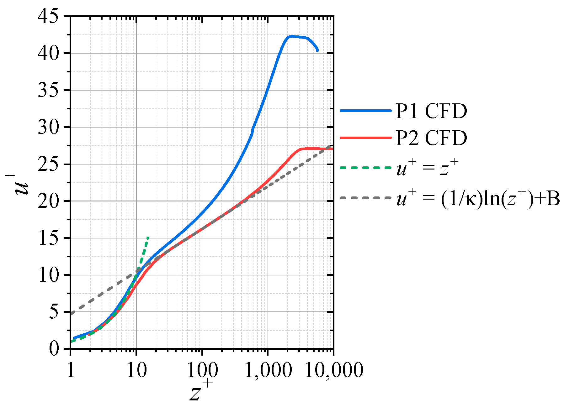
2. Model Setup and Methodology Validation

Examples of blade antennas and pitot tubes used on modern large commercial airliners are shown in Figure 1. Several blade antennas and pitot tubes of various sizes are simultaneously utilized on one airliner. More outline parameters of these two parts produced by different suppliers are summarized in

Table 1. Summary of some representative blade antennas and pitot tubes with applications in airliners and contour parameters. Data from Internet.

Type 1	Supplier	Aircraft	${\mathit{M}\mathit{a}}_{\mathbf{c}\mathbf{r}\mathbf{u}\mathbf{i}\mathbf{s}\mathbf{e}}$	$\mathit{\phi }$	$\mathit{c}\mathit{o}\mathit{s}\left(\mathit{\phi }\right)$	$\mathit{A}\mathit{R}$
S65-8280-18 BA	Sensor Systems Inc., Chatsworth, CA, USA			+46°	0.694659	1.09
20-200-20 BA	Chelton Ltd., Marlow, UK			+45°	0.707107	1.16
110-337 BA	ACR Artex, Fort Lauderdale, FL, USA			+38°	0.788011	0.83
ANT500 BA	Mc Murdo Group, Lanham, MD, USA			+37°	0.798636	1.15
S65-8262-305 BA	Sensor Systems Inc., Chatsworth, CA, USA			+36°	0.809017	1.4
20-200-F18LP BA	Chelton Ltd., Marlow, UK			+30°	0.866025	1.89
21-30-176 BA	Cooper Antennas Ltd., Marlow, UK			+30°	0.866025	1.2
0851HLAI PT	Aero-Instruments, Depew, NY, USA	A320	0.785	−25°	0.906308	1
0851HT1AI PT	AeroControlex, South Euclid, OH, USA	B737	0.74	−25°	0.906308	1
0856AE19AI PT	AeroControlex, South Euclid, OH, USA	B737NG	0.785	−35°	0.819152	1.5
0851FJ1AI PT	Aero-Instruments, Depew, NY, USA	B757	0.8	−35°	0.819152	0.7
PT	--	B747	0.85	−45°	0.707107	1

¹ BA stands for blade antenna and PT stands for pitot tube.

, where the backward sweep angle is positive and the forward sweep angle is denoted by a negative angle. According to Figure 1 and Table 1, blade antennas used in large passenger aircraft generally have a sweep angle ($\phi$) of more than 30° and an aspect ratio ($AR$) of about 1.5. Furthermore, blade antennas typically feature distinctive wing tip sharpening. It is noticed that aircraft models with faster cruising speeds are more likely to use antennas with larger sweep angles. Pitot tubes generally have a forward-swept strut with a probe mounted at the tip. The strut aspect ratio is generally less than 1.5, and the sweep angle is related to the cruise Mach number of the suitable aircraft.

In this study, wall-mounted finite-span airfoils with sweep angles were used as models for blade antennas and pitot tube struts. Combined with Table 1, the forward and backward sweep angles of the wall-mounted symmetric airfoils were set as $\phi$ = −35°, −15°, 0°, +15°, and +35° for analysis. Although small sweep angles (±15°) do not appear in real aircraft, they can still be used to demonstrate the transition process between airfoils with a large sweep angle (±35°) and a straight airfoil. The incoming Mach number (${Ma}_{\infty }$) range was set from 0.8 to 0.9. All airfoils had an aspect ratio of 1.5, i.e., the chord length ($c$) was 0.1 m and the span ($L$) was 0.15 m. The airfoil selected for the following calculations was NACA0012. Given the research context of a cruise phase, the sound velocity ($a$) was approximately 300 m/s, achieved by lowering the inlet temperature to 223.15 K during the simulation. The Reynolds number ($Re$), using the chord length as the reference length, was approximately 6.9 × 10⁵ to 7.7 × 10⁵.

Taking a finite-span airfoil with a sweep of $\phi$ = +35° as an example, the model and calculation grid used in this study are illustrated in Figure 2. The calculation grids extend 2$c$ ahead of the bottom airfoil, 50$c$ behind it, 10$c$ on each side (equivalent to 83.3$d$ with an airfoil thickness $d$ = 0.12$c$ = 0.012 m as a reference), and 5c above it, totaling 3.3$L$. The computational grids have a C-H type topology and a grid number of approximately 8.2 million. The boundary conditions for the bottom surface and the model surface were non-slip walls. The downstream boundary was set as the pressure-outlet, while the remaining boundary conditions were defined as the pressure-far-field. The turbulence of the flow was characterized by incorporating a turbulence viscosity ratio of 10 into these two boundary conditions. The height of the first grid layer satisfies $y^{+}$ = 1. The solver selected for this study was Delayed Detached Eddy Simulation (DDES) for its balance between accuracy and computational cost. A numerical simulation was conducted for 0.1 s of physical time after the flow stabilized or formed a periodic pattern to obtain the mean flow field and far-field noise. During the FW-H sound analogy, the sound pressure measurement point was chosen at a height of 0.1 m above the bottom wall, with the leading edge of the airfoil’s bottom surface as the center when observed from above, positioned on a circle with a radius of 5 m, as shown in Figure 3. The downstream direction (i.e., the positive X-axis direction) was designated as 0 degrees, and measurement points were positioned at one-degree intervals counterclockwise to assess the directivity of far-field noise. The angular position of each measurement point is denoted by the angle $\theta$. The sound pressure data at $\theta$ = 90° (corresponding to the point located 5 m away from the side of the airfoil) serve as the reference point for comparing far-field noise levels under various conditions.

The simulation results of the straight airfoil ($\phi$ = 0°) at ${Ma}_{\infty }$ = 0.85 depict the boundary layer of the bottom wall around the model. Figure 4 illustrates the profile of velocity and turbulent kinetic energy ($TKE$) in the boundary layer on the wall at P1, located 0.1$c$ upstream of the leading edge of the airfoil root ($x/c$ = −0.1, $y/c$ = 0), and at P2, situated 1$c$ away from the leading edge on the side ($x/c$ = 0, $y/c$ = 1). The velocity of P1 outside the boundary layer decreased due to the blockage of the model. Since the distance between the model and the front edge of the computational domain was relatively close (2$c$), the boundary layer at P1 was not sufficient to fully develop into a turbulent boundary layer, but it was significantly different from the laminar boundary layer. The $TKE$ at P2 was significantly higher than that at P1, indicating more pronounced turbulence characteristics.

Figure 5 shows the boundary layer structure at P1 and P2 in more detail by illustrating the relationship between the dimensionless velocity $u^{+}$ and the dimensionless wall distance $z^{+}$ at these locations. Due to the small wall shear stress at point P1, the $u^{+}$ outside the boundary layer is higher here. The boundary layer at P1 already exhibits some characteristics of a turbulent boundary layer, particularly the viscous sublayer with $z^{+}$ < 5. However, the outer part does not adhere to the logarithmic law. The numerical results of the boundary layer at P2 align well with the predicted characteristics of turbulent boundary layer theory, both in the viscous sublayer ($z^{+}$ < 5) and the log-law layer (30 < $z^{+}$ < 300). In the two intervals, the maximum difference of $u^{+}$ between the simulation results and the theoretical prediction is approximately 0.2. The error rate does not exceed 5% at $z^{+}$ = 5 and is even smaller at other locations. By comparing the boundary layer of the two locations, it is evident that the boundary layer surrounding the model transitions into a turbulent boundary layer due to the model’s influence. This observation suggests that the flow dynamics in the junction are primarily influenced by the model. Although the configuration and thickness of the boundary layer may numerically affect the flow and noise at the junction, their impact on the flow mechanism is limited.

The experimental data from the ONERA M6 supercritical wing were used to assess the numerical method’s capability to accurately predict the shock position on the wing surface under transonic conditions [38,39]. By employing a grid with a similar meshing method and grid number as the grids used in symmetric airfoils for the simulation of the M6 wing, the bottom boundary condition was set as symmetry in this case. The comparison of the numerical simulation and experimental results for the test Case 2308 (incoming Mach number ${Ma}_{\infty }$ = 0.84, angle of attack AoA = 3.06°, Reynolds number based on chord length of bottom ${Re}_{\mathrm{c}\_\mathrm{r}\mathrm{o}\mathrm{o}\mathrm{t}}$ = 14.6 × 10⁶, and far-field temperature $T_{\infty }$ = 300 K; this case fell within the research scope of this study [38]) is shown in Figure 6. It can be seen that the numerical method can accurately capture both the suction peak and the shock wave position under this condition. Since the angle of attack in this study was maintained at 0°, it can be considered that the numerical method met the research requirements.

Given that the angle of attack is 0° in this investigation, the phenomena on either side of the airfoil exhibit statistical symmetry. Consequently, the subsequent analysis does not differentiate between the suction surface and the pressure surface.

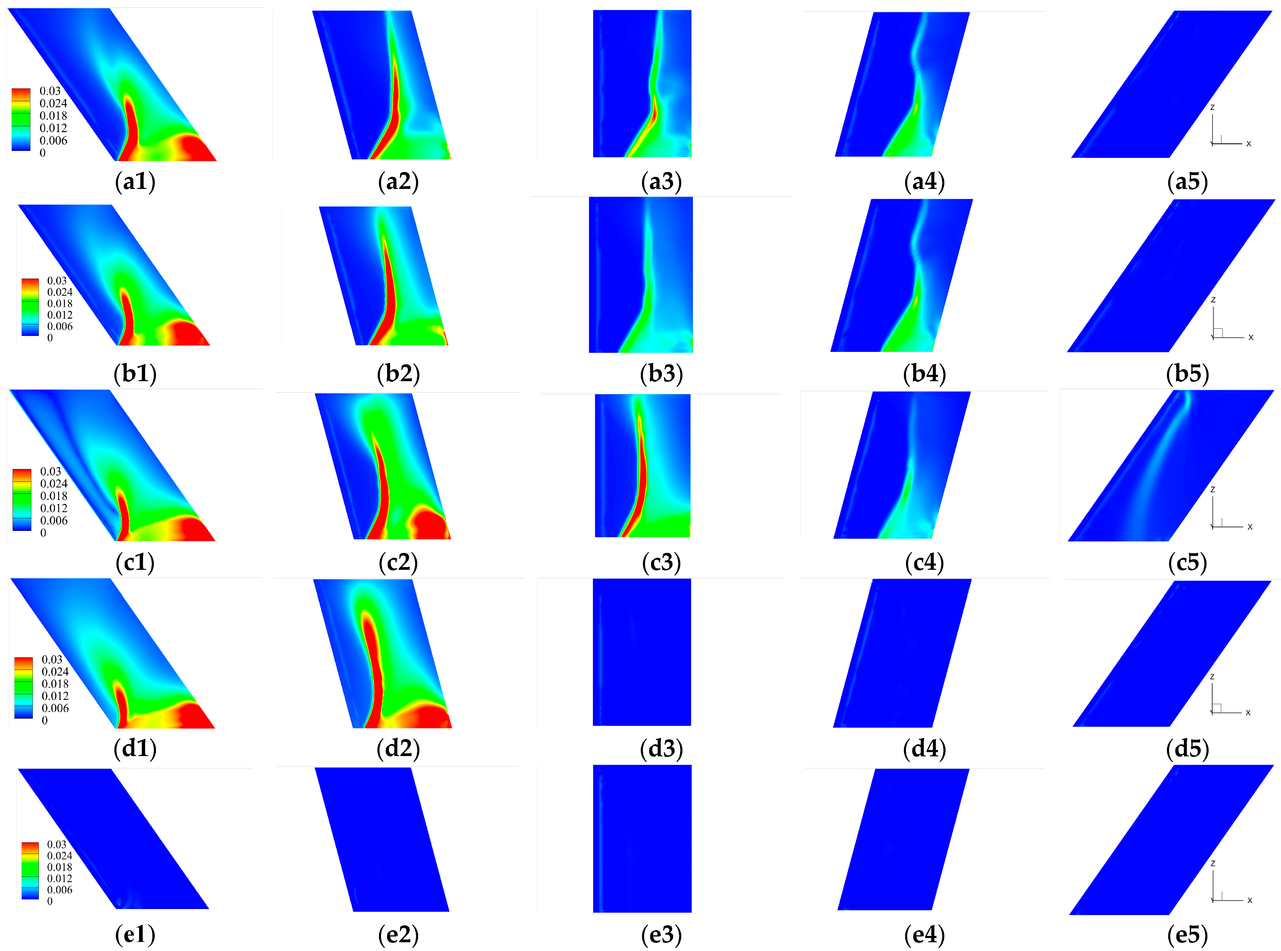
3. The Effect of Sweep Angle on Shock Waves Position, Pressure Fluctuations, and Bottom Boundary Layer

In transonic flow, particular emphasis must be placed on the precise location of shock waves and the separation of the boundary layer on the surface of the wall. These concerns are closely associated with fluctuations in surface pressure and the production of noise. Figure 7 displays the instantaneous simulation results of the surface streamlines and the shock wave positions for a wall-mounted finite span with different sweep angles within the range of ${Ma}_{\infty }$ = 0.8~0.9. The shock position is represented by the purple iso-surface of ${\displaystyle \frac{U}{a}}·{\displaystyle \frac{\nabla p}{‖\nabla p‖}}$ = 16. This quantity takes into account both the local Mach number and the pressure gradient, and it has a large value near the shock wave. The iso-surface value ‘16′ was carefully adjusted so that the position of the iso-surface corresponded to areas of high shock wave intensities. Nevertheless, it should be noted that the shock wave is not limited exclusively to the area enclosed by the iso-surface. The region enclosed by the iso-surface serves to define both the location and strength of the shock wave. It can be observed that the strength of shock waves increases with ${Ma}_{\infty }$. The shock wave generated by forward-swept airfoils initially appears at the junction and progresses towards the midspan as ${Ma}_{\infty }$ increases. In contrast, the shock wave produced by backward-swept airfoils originates at the tip and extends towards the midspan with the increasing ${Ma}_{\infty }$.

For each swept angle airfoil, the intensity of surface shock waves increases with a rise in the ${Ma}_{\infty }$. Additionally, the direction of the shock wave is streamwise-associated with both ${Ma}_{\infty }$ and $\phi$ simultaneously. In airfoils with $\phi$ = −35°, the shock wave predominantly localizes at the junction between the root and the bottom wall. Notably, under conditions where ${Ma}_{\infty }$ ≥ 0.825, a distinct separation flow emerges within this junction. For airfoils with $\phi$ = −15°, flow separation at the junction also transpires within this ${Ma}_{\infty }$ range, and the shock wave exhibits higher intensity in the midspan of the airfoil. When ${Ma}_{\infty }$ ≥ 0.85, a flow separation of the junction part of the straight airfoil ($\phi$ = 0°) takes place, and surface flow separation and a reattachment phenomenon behind the shock wave in the midspan occur when ${Ma}_{\infty }$ is higher. For the airfoil with $\phi$ = +15°, the shock wave intensity is slightly higher at the airfoil surface, and flow separation does not happen at the junction until ${Ma}_{\infty }$ ≥ 0.875. The separation at the junction part of the previous airfoils extends to the trailing edge. The shock waves observed on the airfoil surface at $\phi$ = +35° primarily appear near the tip part within the ${Ma}_{\infty }$ range of 0.8 to 0.9. When ${Ma}_{\infty }$ approaches 0.9, flow separation and reattachment phenomena occur behind the shock waves at the tip of the airfoil, exhibiting a minimal separation distance. Due to the characteristics of the junction and the tip, forward- and backward-swept airfoils with the same absolute value of sweep angle exhibit distinct separation patterns at identical ${Ma}_{\infty }$. This difference is also reflected in pressure fluctuations on the airfoil surface. The root-mean-square surface pressure coefficient ($C_{P\mathrm{r}\mathrm{m}\mathrm{s}}$) of airfoils with different sweep angles at ${Ma}_{\mathrm{\infty }}$ = 0.8~0.9 is illustrated in Figure 7. This value represents the local pressure fluctuation, and the fluctuations near the shock wave indicate the motion of the shock wave’s position. When ${Ma}_{\mathrm{\infty }}$ = 0.8, the surface pressure fluctuations of the airfoil surfaces with a forward/backward sweep angle are negligible, and the straight airfoil surface does not exhibit high pressure fluctuation areas corresponding to the motion of the shock wave, while only a region with a relatively high $C_{P\mathrm{r}\mathrm{m}\mathrm{s}}$ value of about 0.005 extends near the leading edge of the straight airfoil. The pressure fluctuations near the leading edge are associated with a normal Mach number, so they only appear on the straight airfoil when ${Ma}_{\mathrm{\infty }}$ is relatively small. The airfoils with $\phi$ = ± 15° begin to exhibit noticeable leading-edge pressure fluctuations at ${Ma}_{\mathrm{\infty }}$ = 0.825, while airfoils with $\phi$ = ±35° show this phenomenon at ${Ma}_{\mathrm{\infty }}$ = 0.85. The pressure fluctuations at the leading edge may result from the flow being deflected from the airfoil, a phenomenon associated with monopole noise. Such noise is positively correlated with ${Ma}_{\mathrm{\infty }}$.

By comparing Figure 7 with Figure 8, the range of ${Ma}_{\mathrm{\infty }}$ and $\phi$ where the shock motion occurs can be defined. When $\phi$ = −35° and −15°, the shock position occurs at ${Ma}_{\mathrm{\infty }}$ ≥0.825; when $\phi$ = 0°, ${Ma}_{\mathrm{\infty }}$ ≥ 0.85; and when $\phi$ = +15°, ${Ma}_{\mathrm{\infty }}$ ≥ 0.875. At the same sweep angle, the intensity of pressure fluctuation is not strictly positively correlated with Mach number. For the $\phi$ = 0° airfoil, the pressure fluctuation is most noticeable when ${Ma}_{\mathrm{\infty }}$ = 0.85, followed by ${Ma}_{\mathrm{\infty }}$ = 0.90, and then when ${Ma}_{\mathrm{\infty }}$ = 0.875. For the $\phi$ = +35° airfoil, the pressure fluctuation caused by the movement of the shock wave position is noticeable only when ${Ma}_{\mathrm{\infty }}$ = 0.85. For the $\phi$ = −15° airfoil, the pressure fluctuation intensity decreases even further as ${Ma}_{\mathrm{\infty }}$ increases when ${Ma}_{\mathrm{\infty }}$ ≥ 0.825. In addition to the Mach number itself, the relative chordwise position of the shock wave also affects the intensity of the pressure fluctuation. Another common observation is that when the shock wave position shifts near the airfoil root, a significant pressure fluctuation area forms behind the shock wave, especially close to the trailing edge. This suggests that the boundary layer separation and vortex shedding phenomena occur at the junction following a shock wave. The intense pressure fluctuations on the airfoil surface can create a dipole sound source.

The separation of the junction area involves SWBLIs. To provide a more intuitive representation of boundary layer separation, Figure 9 illustrates the iso-surface of $k’={\displaystyle \frac{1}{2}}\left({u\prime }^2+{v^{\prime }}^2+{w\prime }^2\right)$ ($u^{\prime }$, $v^{\prime }$, and $w^{\prime }$ represent the fluctuation velocity, which is the difference between the instantaneous velocity and the time-averaged velocity in the $x$, $y$, and $z$ directions) and streamlines near the junction area of ${Ma}_{\mathrm{\infty }}$ ≥ 0.85 and $\phi$ ≤ +15°. For reference, the iso-surface depicting the same shock position as shown in Figure 7 is also presented in Figure 9. Under the same ${Ma}_{\mathrm{\infty }}$, the trend in the shock location at the root area moving backward with an increase in the sweep angle is more obvious in Figure 9. In comparison to the case with ${Ma}_{\mathrm{\infty }}$ = 0.85 and $\phi$ = +15° where there is no boundary layer separation at the bottom of the junction area, the shock waves on the airfoil surface and the bottom wall of other cases are all λ-type, and a “tetrahedral region” is formed at the shock position of the junction area. Additionally, the turbulent kinetic energy in the junction area starts to increase from the upstream shock wave branch, and a noticeable flow separation phenomenon behind the downstream branch. In addition to the separation region within the junction area, another region where elevated turbulent kinetic energy is observed is at the location of the shock wave. The unsteady flow observed in this region is primarily attributed to the motion of the shock wave. It can be concluded that when the shock wave position remains stationary, boundary layer separation does not occur after the shock wave. With an increase in ${Ma}_{\mathrm{\infty }}$, the range of obvious $k’$ will also expand. The airfoil with sweep angles of 0° and −15° also showed an increase in turbulent kinetic energy at ${Ma}_{\mathrm{\infty }}$ = 0.9. However, for $\phi$ = −35°, significant $k’$ appeared only near the bottom wall. This suggests that a greater forward sweep angle encourages boundary layer separation after the shock wave position at the junction, while restricting separation on the airfoil surface to the root area.

Part of the statistical characteristics of turbulence in the $y/c$ = −0.1 plane of the cases discussed in the above paragraph are depicted in Figure 10, Figure 11, Figure 12 and Figure 13 to illustrate the influence of SWBLIs on the flow field. The root mean square of flow velocity ($u_{\mathrm{r}\mathrm{m}\mathrm{s}}$, which is normalized by dividing $u_{\mathrm{\infty }}$) in this plane represents the change in shock position, and the shedding of the underlying boundary layer is shown in Figure 10. The isograms in the figure represent time-averaged Mach numbers. Reynolds shear stresses in the three directions ($\overline{u^{\prime }{v}^{\prime }}$, $\overline{u^{\prime }{w}^{\prime }}$, and $\overline{v^{\prime }{w}^{\prime }}$, which are normalized by dividing $u_{\mathrm{\infty }}^2$) in the plane are shown in Figure 11, Figure 12 and Figure 13, respectively. It can be seen that ${Ma}_{\mathrm{\infty }}$ has no significant effect on the distribution of Reynolds stress in the range depicted. The $\overline{u^{\prime }{v}^{\prime }}/u_{\mathrm{\infty }}^2$ stress is influenced by compression and expansion around the airfoil. It is more pronounced in the wake originating from the tip area but less obvious in the shock area. The $\overline{u^{\prime }{w}^{\prime }}/u_{\mathrm{\infty }}^2$ stress mainly concentrates in two areas: the leading edge of the tip and the triangular area between the two branches of the λ-type shock wave and above the separation area. When the airfoil has a forward-swept angle, the $\overline{u^{\prime }{w}^{\prime }}/u_{\mathrm{\infty }}^2$ stress extends across the leading edge of the airfoil, and the strength is concentrated at the bottom. The $\overline{v^{\prime }{w}^{\prime }}/u_{\mathrm{\infty }}^2$ stress has a similar distribution, although its strength is only evident at the separation point on the bottom, then fills the triangular area like the $\overline{u^{\prime }{w}^{\prime }}/u_{\mathrm{\infty }}^2$ stress. In addition, various stresses are more pronounced at the edge of the separation area, specifically at the interface with the outer layer flow, forming a wake near the bottom surface, while the stresses within the separation area are less prominent. In summary, the forward-swept angle causes the SWBLIs at the bottom junction area, leading to an increase in the Reynolds stress in this region.

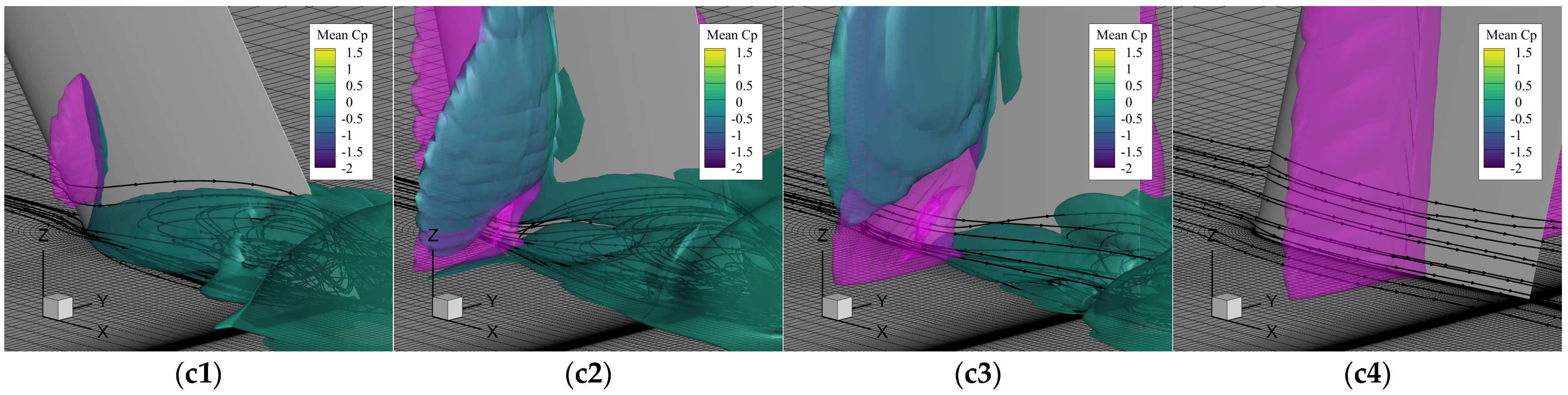
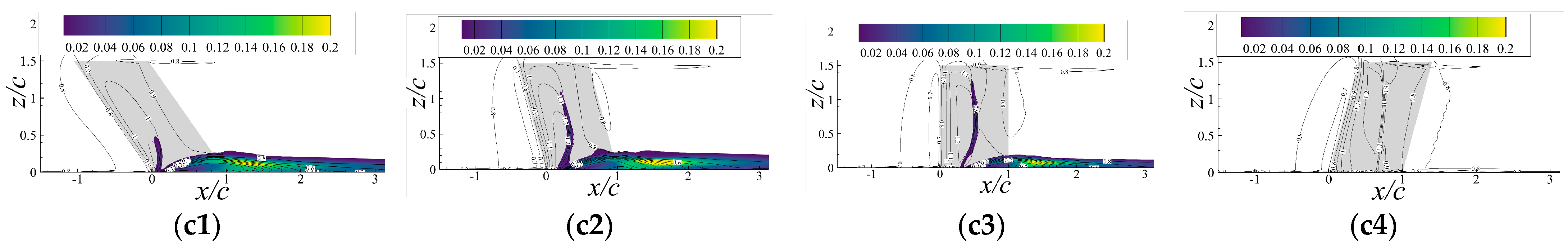
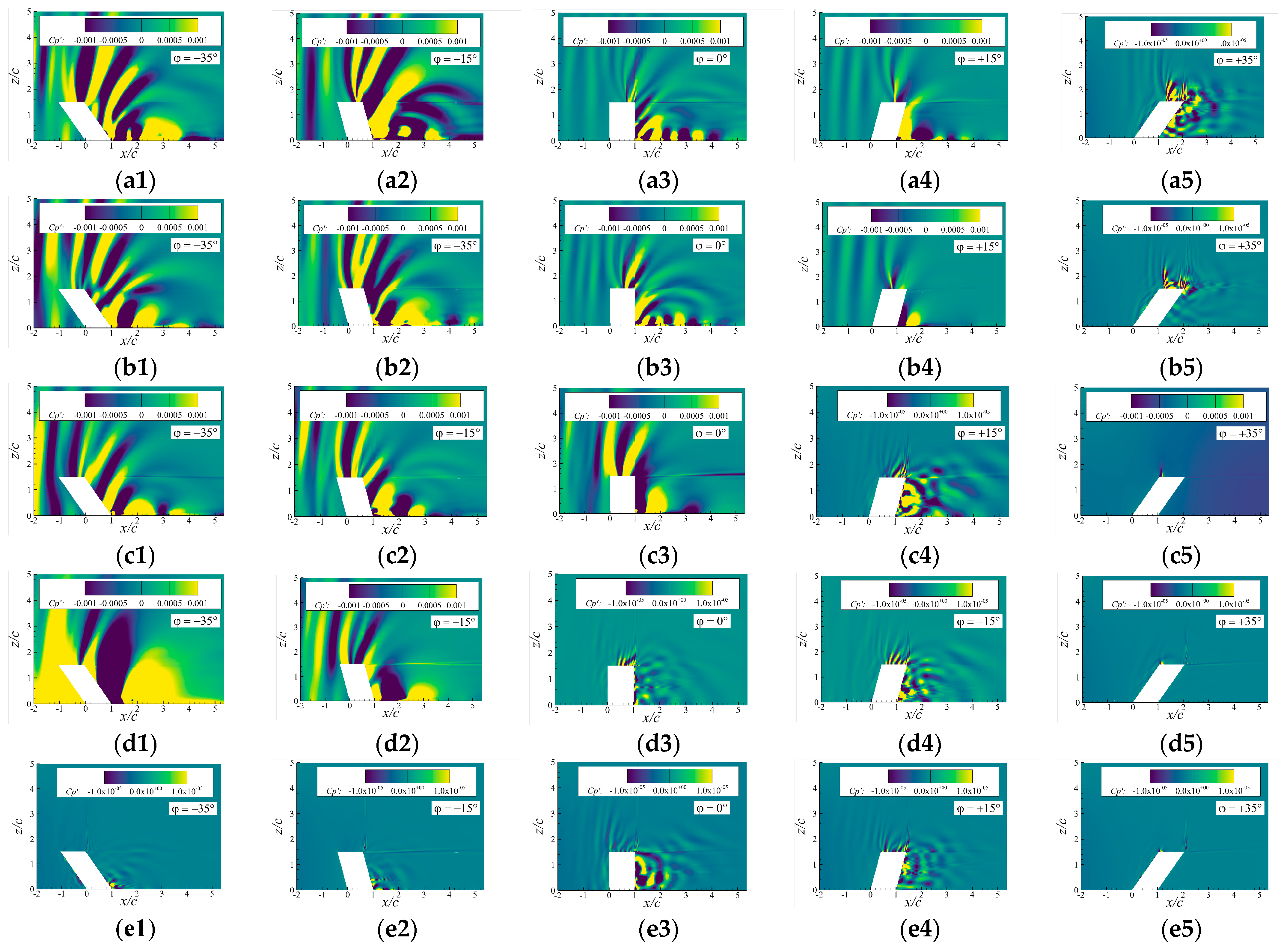
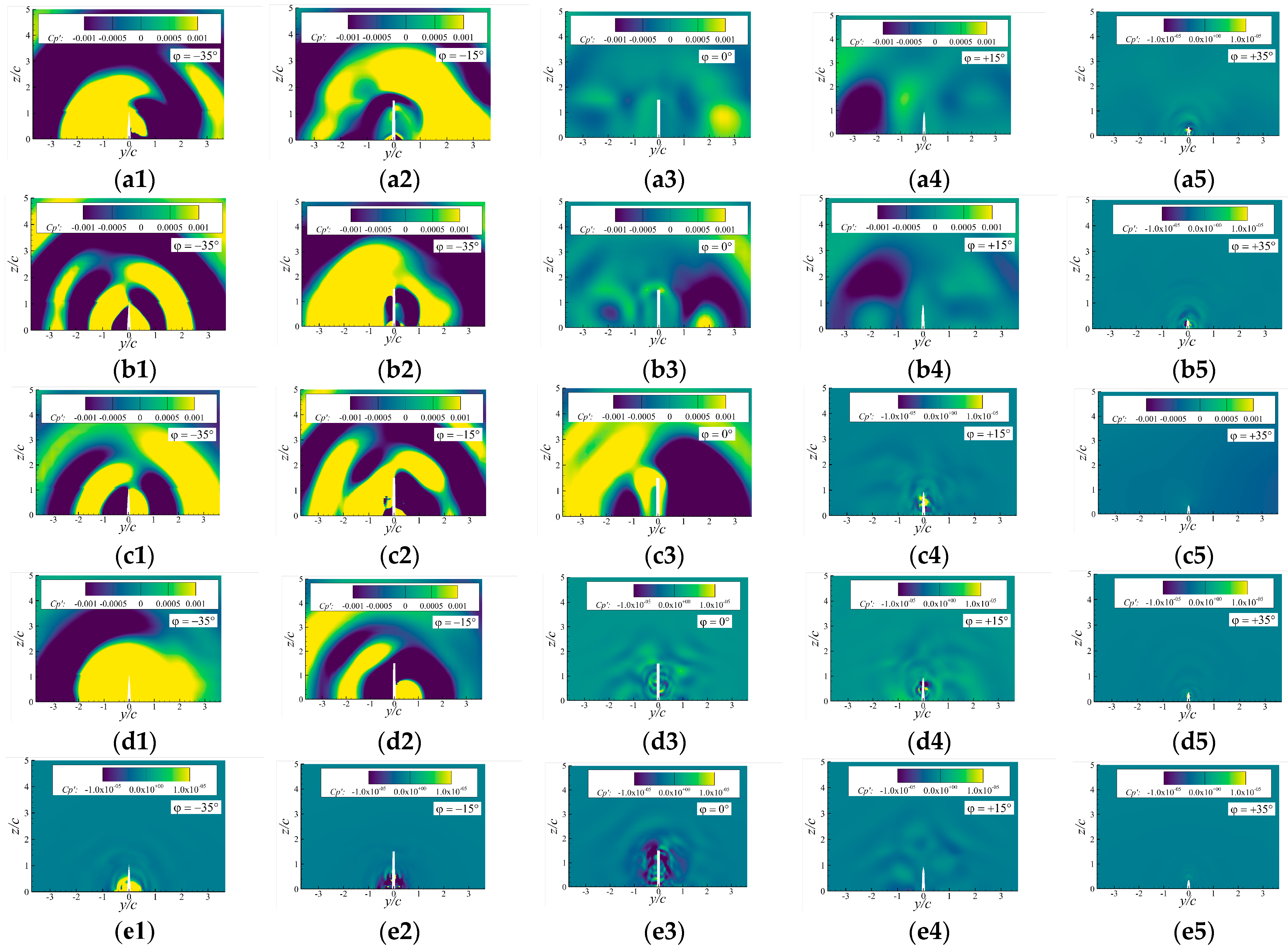
4. Pressure Wave Propagation of Near Field

In this section, the instantaneous pressure fluctuation coefficient (${C_P}^{\prime }=2(p-\overline{p})/\rho U_{\mathrm{\infty }}^2$) is used to reflect the pressure wave propagation and sound field in the near field. The illustration of ${C_P}^{\prime }$ near the bottom wall ($z/c$ = 0.1), in the longitudinal ($y/c$ = 0) and streamwise ($x/c$ = 0.025) sections, are presented in Figure 14, Figure 15 and Figure 16.

Due to the significant difference in pressure amplitude under various conditions, two kinds of ranges of ${C_P}^{\prime }$ are used based on the presence of a noticeable motion of the shock wave position, large amplitude, and small amplitude. Figure 14 ($z/c$ = 0.1) illustrates the pressure wave propagation in the boundary layer of the bottom wall, showing the propagation of pressure waves around the airfoil. It can be seen that the tendency of the shock position is towards the trailing edge as ${Ma}_{\mathrm{\infty }}$ increases. For small pressure fluctuation conditions without SWBLIs, the primary direction of sound propagation is towards the downstream direction, while the amplitude of the pressure wave in front of the shock wave is very small. The boundary layer behind the shock wave becomes more turbulent, and the pressure fluctuation is positively correlated with the normal Mach number. For significant pressure fluctuation cases with SWBLIs, the presence of discernible pressure waves propagates upstream ahead of the shock wave. These pressure waves result from the back and forth of the shock wave position. The pressure wave is reflected by the wall surface between the shock wave and the trailing edge, propagating to both the upper and lower sides in an oblique waveform. This may explain why the boundary layer at P2 exhibits significant turbulent characteristics. At the trailing edge, pressure waves propagate in downstream directions as a result of the shedding of alternating vortices, whereas pressure waves propagate circumferentially. The aforementioned phenomena show a positive correlation with the surface $C_{P\mathrm{r}\mathrm{m}\mathrm{s}}$.

In the longitudinal slice ($y/c$ = 0), as shown in Figure 15, the propagation characteristics of pressure waves in a spanwise direction by the sweep angle is shown. For cases without SWBLIs, turbulence occurs only near the bottom wall when $\phi$ < 0°, while the fluctuation at the trailing edge in the midspan and tip area is very weak. On the other hand, both the straight airfoil and the $\phi$ = +15° airfoil exhibit pressure fluctuations at the trailing edge along the full span for the non−shock−motion cases. This demonstrates that the forward sweep angle can limit the turbulence intensity in the junction area. When $\phi$ = +35°, the pressure fluctuation appears at the trailing edge of the tip part when ${Ma}_{\mathrm{\infty }}$ < 0.85, and with an increase in ${Ma}_{\mathrm{\infty }}$, the development shifts towards the midspan of the airfoil. For the cases with SWBLIs, pressure fluctuations near the bottom wall of forward−swept airfoils are shown to propagate along the spanwise direction, resulting in significant pressure fluctuations above the tip, while for the straight airfoil and the airfoil with $\phi$ = +15°, the propagation of the pressure wave along the airfoil is suppressed, resulting in relatively weak pressure fluctuations above the tip. This phenomenon could be attributed to the low intensity of pressure fluctuation within the boundary layer under these conditions, or the difficulty for the pressure wave to propagate vertically when $\phi$ ≥ 0°. In summary, the forward−swept angle inhibits the longitudinal propagation of the pressure wave in the absence of SWBLIs, and enhances it in the presence of SWBLIs. In particular, in the case of a backward−swept airfoil with $\phi$ = +35° and ${Ma}_{\mathrm{\infty }}$ = 0.85, noticeable pressure fluctuations are observed near the shock wave location at the tip area. Conversely, minimal pressure fluctuations were detected near the bottom surface of the airfoil. Since this study focuses on the attachment of the fuselage surface under the cruise phase, the sound propagation above the tip corresponds to the noise propagating outside the cabin and will not be discussed further.

Figure 16 illustrates the instantaneous pressure fluctuations in a plane perpendicular to the streamwise direction ($x/c$ = 0.025, where the airfoil’s bottom thickness is maximum). For cases without obvious SWBLIs, there are only insignificant pressure waves. Except for the upward propagation tendency of pressure waves when $\phi$ = +35°, there is no obvious propagation direction around airfoils with other sweep angles. For cases with obvious SWBLIs, there are very intense pressure waves in this plane. Some images exhibit distinct ripples, while others display large areas in phase around the airfoils. This reflects the characteristics of the oblique forward propagation of pressure waves in this region. For the straight airfoil and the $\phi$ = +15° airfoil, the amplitude is smaller than that of other cases with large amplitudes when ${Ma}_{\mathrm{\infty }}$ = 0.875 and 0.90, indicating that the pressure wave propagating forward under these conditions is relatively weak. In these cases, it can also be observed that the pressure propagation near the bottom surface is stronger than the pressure propagation in the other directions. The bottom wall of the attachments on the aircraft surface exhibits a specific curvature in reality, as opposed to being flat. However, the size of the attachments is significantly smaller in comparison to the curvature of the fuselage. The phenomena discussed in this section continue to hold significance.

In conclusion, taking the above results into consideration, when the shock wave position moves on the airfoil’s surface, the sound wave mainly propagates to both sides and upstream. When the airfoil has a forward−swept angle, the pressure fluctuation propagating upstream is more pronounced.

5. Far-Field Noise Directivity

5.1. Effect of Forward and Backward Sweep Angles on Far-Field Noise Directivity

In order to demonstrate the influence of the forward and backward sweep angle $\phi$ on far-field noise directivity, the overall sound pressure level (OASPL) for airfoils with different values of $\phi$ in the $\theta$ = 90° direction under the same ${Ma}_{\mathrm{\infty }}$ is shown in Figure 17a.

When ${Ma}_{\mathrm{\infty }}$ = 0.8, the pressure fluctuation on the airfoil surface is small due to the low inflow velocity, and the noise is primarily influenced by the normal Mach number. Therefore, the straight airfoil exhibits the highest OASPL. At this time, airfoils with the same absolute value of $\phi$ exhibit closer OASPL. It is worth noting that the far-field noise of airfoils with a larger sweep angle is more pronounced than that of airfoils with a smaller sweep angle. This suggests that $\phi$ itself contributes to an increase in far-field noise at this Mach number. When ${Ma}_{\mathrm{\infty }}$= 0.8, the OASPL of each airfoil is generally low.

However, with an increase in ${Ma}_{\mathrm{\infty }}$, the far-field noise level significantly rises, with a maximum increase of about 35 dB at $\phi$ = −15°. Compared with Figure 7, it can be observed that this noise is associated with a fluctuation in airfoil surface pressure caused by the motion of the shock wave position and separated flow in the junction area. In order to quantitatively measure the pressure fluctuation on the airfoil surface, $C_{P\mathrm{r}\mathrm{m}\mathrm{s}}$ is integrated over the airfoil surface and normalized by the reference area of the airfoils, i.e., the normalized airfoil surface pressure fluctuation equals ${\displaystyle \frac{1}{2S_{\mathrm{r}\mathrm{e}\mathrm{f}}}}∯C_{P\mathrm{r}\mathrm{m}\mathrm{s}}\mathrm{d}A$, and here $S_{\mathrm{r}\mathrm{e}\mathrm{f}}=cL=$ 0.015 m² is the reference area of the airfoils, which is doubled for both sides of the airfoils, and $\mathrm{d}A$ is the area element of the airfoil surface. The result of normalized airfoil surface pressure fluctuation is shown in Figure 17b. Comparing the far-field noise level with the airfoil surface pressure fluctuation, it can be found that they exhibit a similar variation trend with $\phi$. This indicates that the pressure fluctuation on the airfoil surface plays a significant role as a source of far-field noise. When ${Ma}_{\mathrm{\infty }}$ = 0.825 and 0.85, the airfoil with a $\phi$ of −15° exhibits the most noticeable surface pressure pulsation and far-field noise, followed by the airfoil with a $\phi$ of −35°. When ${Ma}_{\mathrm{\infty }}$ = 0.875 and 0.90, the noise and surface pressure fluctuation decreased with the increase in $\phi$. In addition to airfoil surface pressure fluctuations, Mach number also contributes to far-field noise, which will be discussed in Section 5.2.

Figure 18 illustrates the far-field noise directivity of the airfoil with various forward and backward sweep angles at each ${Ma}_{\mathrm{\infty }}$. In general, the noise directivity curve can take two forms. When the airfoil surface pressure fluctuation is weak and the noise is small, the curve shows evident fluctuations. Conversely, when the pressure fluctuation is obvious and the far-field noise is loud, the curve appears smoother. The far-field noise is more noticeable on both sides ($\theta$ = 90°, 270°), but less so upstream ($\theta$ = 180°) and downstream ($\theta$ = 0°) of the airfoil. Especially when the curve is smooth, the noise in the direction of $\theta$ = 0° hardly changes with $\phi$, demonstrating the directivity characteristic of typical dipole noise. Specifically, when ${Ma}_{\mathrm{\infty }}$= 0.80, the curve of $\phi$ = ±35° exhibits less shrinkage in the upstream and downstream directions compared to that of $\phi$ = −15°, 0°, and +15°, which aligns more closely with the distribution pattern of monopole noise. When ${Ma}_{\mathrm{\infty }}$= 0.825, the noise levels of $\phi$ = −35° and −15° are higher downstream, and the retraction of the two curves is most pronounced in that direction. At ${Ma}_{\mathrm{\infty }}$= 0.85, the noise levels of the airfoils at $\phi$ = +15° and +35° are almost identical in the $\theta$ = 90° direction. But behind the airfoil ($\theta$ < 90° and > 270°), the noise at $\phi$ = +15° is greater than that at $\phi$ = +35°, which is consistent with the noise decreasing as $\phi$ increases at higher ${Ma}_{\mathrm{\infty }}$. The noise of the airfoil with a $\phi$ = +35° at $\theta$ = 90° may be slightly increased by the pressure fluctuation at the airfoil tip, causing a slight change in its value compared to when $\phi$ = +15°. At ${Ma}_{\mathrm{\infty }}$ = 0.875 and 0.90, the directivity curve of the straight airfoil ($\phi$ = 0°) also shows evident fluctuations upstream of the airfoil (90° < $\theta$ < 270°), even though the curve as a whole is still closer to the dipole noise. This may be the effect of the larger normal Mach number. In this ${Ma}_{\mathrm{\infty }}$ range, the maximum noise of the most airfoils appears near the $\theta$ = 80° and 280° directions, except for the $\phi$ = +35° airfoil.

5.2. Effect of Forward and Backward Sweep Angles on Far-Field Noise Directivity

The influence of the normal Mach number ${Ma}_{\mathrm{n}}$= ${Ma}_{\mathrm{\infty }}·\cos \phi$ and incoming Mach number ${Ma}_{\mathrm{\infty }}$ on far-field noise will be discussed in this section. The location and strength of shock waves on the airfoil surface are correlated with ${Ma}_{\mathrm{n}}$. The variation in OASPL in the $\theta$ = 90° direction of the airfoil and the normalized integral of fluctuation pressure on the airfoil surface for each $\phi$ against ${Ma}_{\mathrm{n}}$ is shown in Figure 19. It can be observed that the far-field noise tends to increase with an increase in ${Ma}_{\mathrm{n}}$, but it is not monotonous for each $\phi$. The far-field noise increases with the magnitude of pressure fluctuations on the airfoil surface. Moreover, the surface pressure fluctuation and far-field noise OASPL tend to concentrate as ${Ma}_{\mathrm{n}}$ increases for airfoils with varying $\phi$. As ${Ma}_{\mathrm{n}}$ approaches 0.9, there is a decrease in the integral of $C_{P\mathrm{r}\mathrm{m}\mathrm{s}}$ on the airfoil surface. It can be seen by comparing Figure 19a,b that, apart from the impact of pressure fluctuation on the airfoil surface, the far-field noise is likely to escalate with the ${Ma}_{\mathrm{n}}$.

The influence of ${Ma}_{\mathrm{\infty }}$ on the far-field noise directivity of the airfoils at each $\phi$ is illustrated in Figure 20. From the results of $\phi$ = −35° and +15°, it can be seen that the amplitude of far-field noise increases with ${Ma}_{\mathrm{\infty }}$. When $\phi$ is −15° and 0°, the far-field noise generated by the significant pressure fluctuation in the midspan of the airfoil is significantly larger than the noise when the surface pressure fluctuation is not significant at smaller ${Ma}_{\mathrm{\infty }}$. However, if the noise mechanism does not change, the influence of ${Ma}_{\mathrm{\infty }}$ on the noise level in the current range is minor and weaker than that of $\phi$. In the image of $\phi$ = +35°, the far-field noise distribution of the monopole feature is very noticeable when ${Ma}_{\mathrm{\infty }}$ = 0.80.

6. Conclusions

In this study, numerical simulations were conducted to analyze the flow-field and far-field noise directivity of a wall-mounted finite span symmetric airfoil with forward and backward sweep angles ranging from −35° to +35° and an aspect ratio of 1.5 under transonic incoming flow conditions with ${Ma}_{\mathrm{\infty }}$ = 0.8~0.9. The results indicate that the shock position, instantaneous streamline, pressure fluctuation on the airfoil surface, and far-field noise directivity are influenced by the sweep angle $\phi$ and ${Ma}_{\mathrm{\infty }}$. When flow separation occurs in the junction area between the airfoil and the bottom wall, the shock wave structure transforms into an λ-type configuration, causing the shock wave position to oscillate between moving backwards and forwards. These appearances result in significant fluctuations in surface pressure, which manifest as noticeable dipole noise in the far field. The forward sweep angle results in an increased shock wave intensity at the root area, leading to an earlier separation of the junction area at lower ${Ma}_{\mathrm{\infty }}$. The backward sweep angle of the airfoil will attenuate the intensity of the shock wave, impede flow separation, and reduce noise generation. The primary findings of this research are summarized as follows:

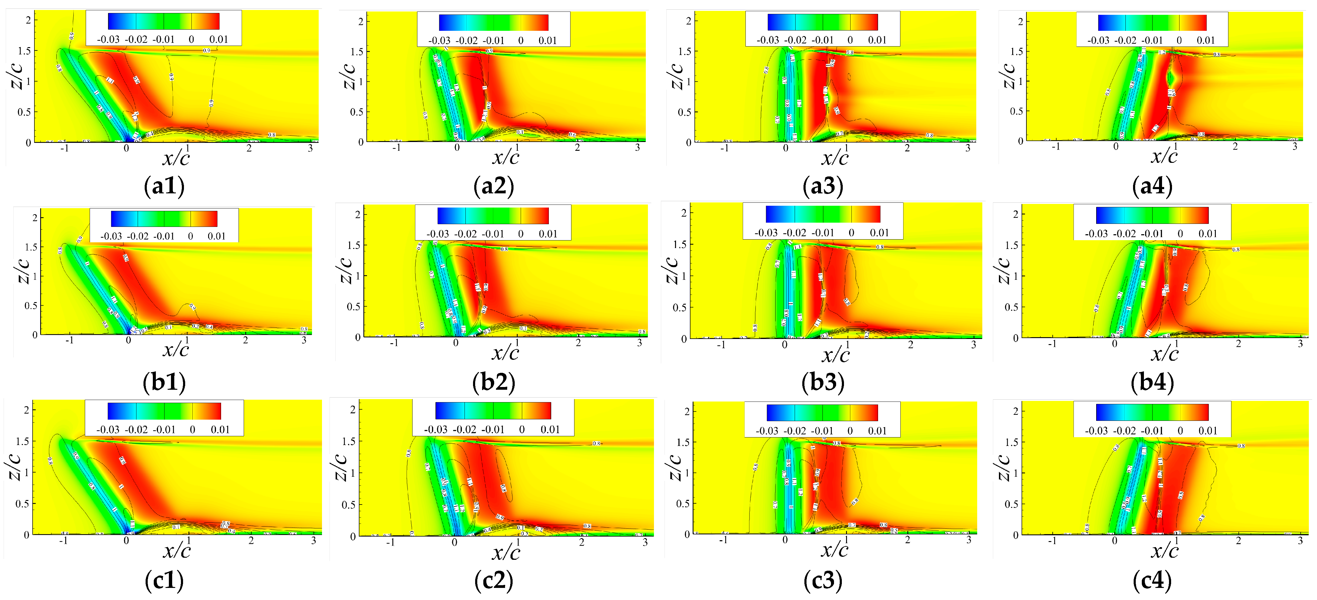
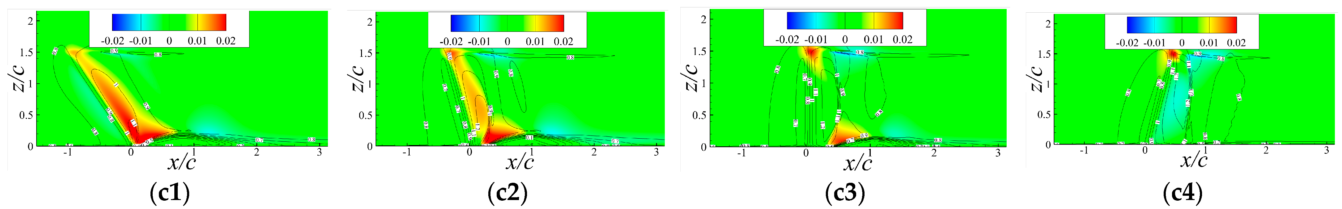
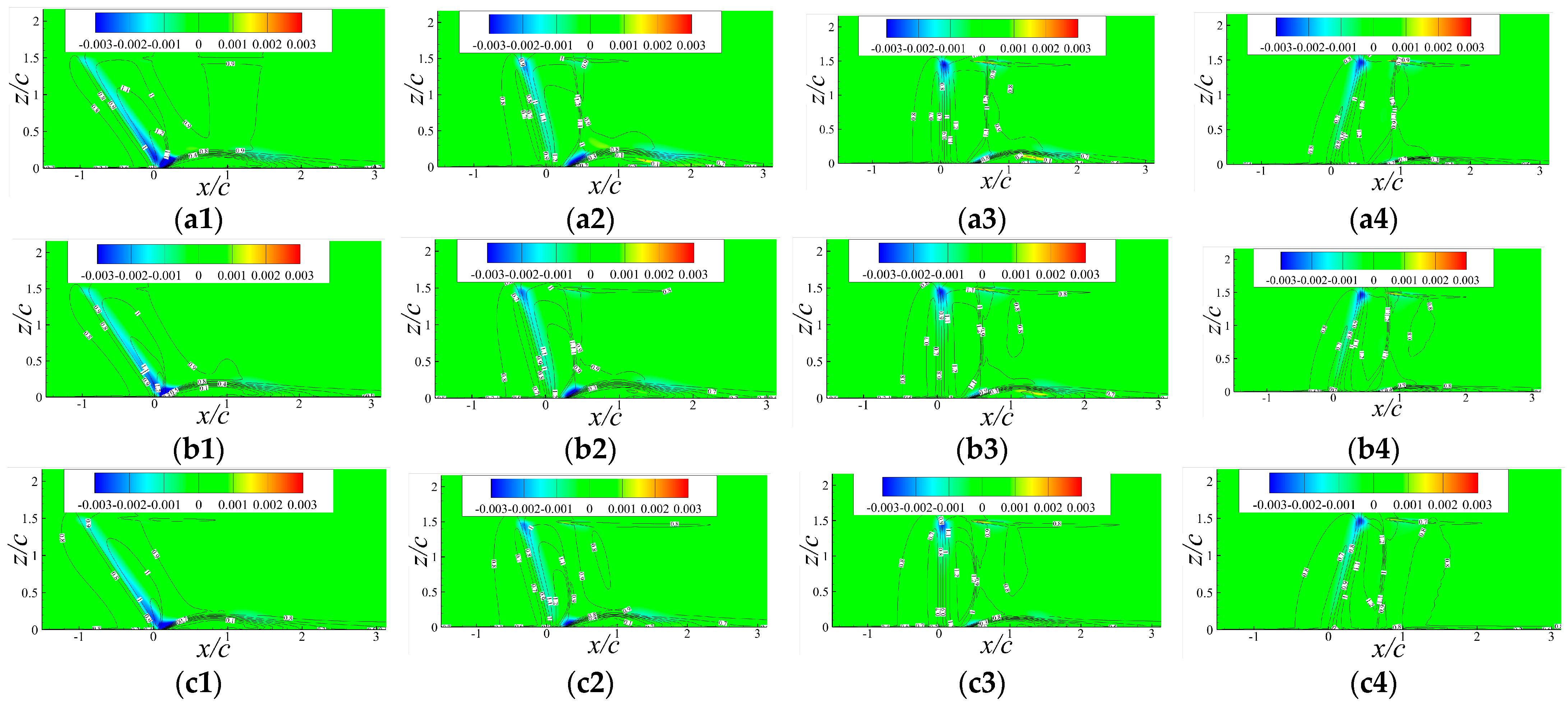
• The airfoil surface pressure fluctuation caused by the motion of the shock wave position in the junction area occurs at ${Ma}_{\mathrm{\infty }}$ ≥ 0.825 for the airfoils with $\phi$ = −35° and −15°, at ${Ma}_{\mathrm{\infty }}$ ≥ 0.85 for the airfoils with $\phi$ = 0°, and at ${Ma}_{\mathrm{\infty }}$ ≥ 0.875 for the airfoils with $\phi$ = +15°. When $\phi$ = +35°, the airfoils do not produce flow separation at the junction. Instead, there is only a relatively weak pressure fluctuation at the tip area at ${Ma}_{\mathrm{\infty }}$ = 0.85 for the airfoil of $\phi$ = +35°.
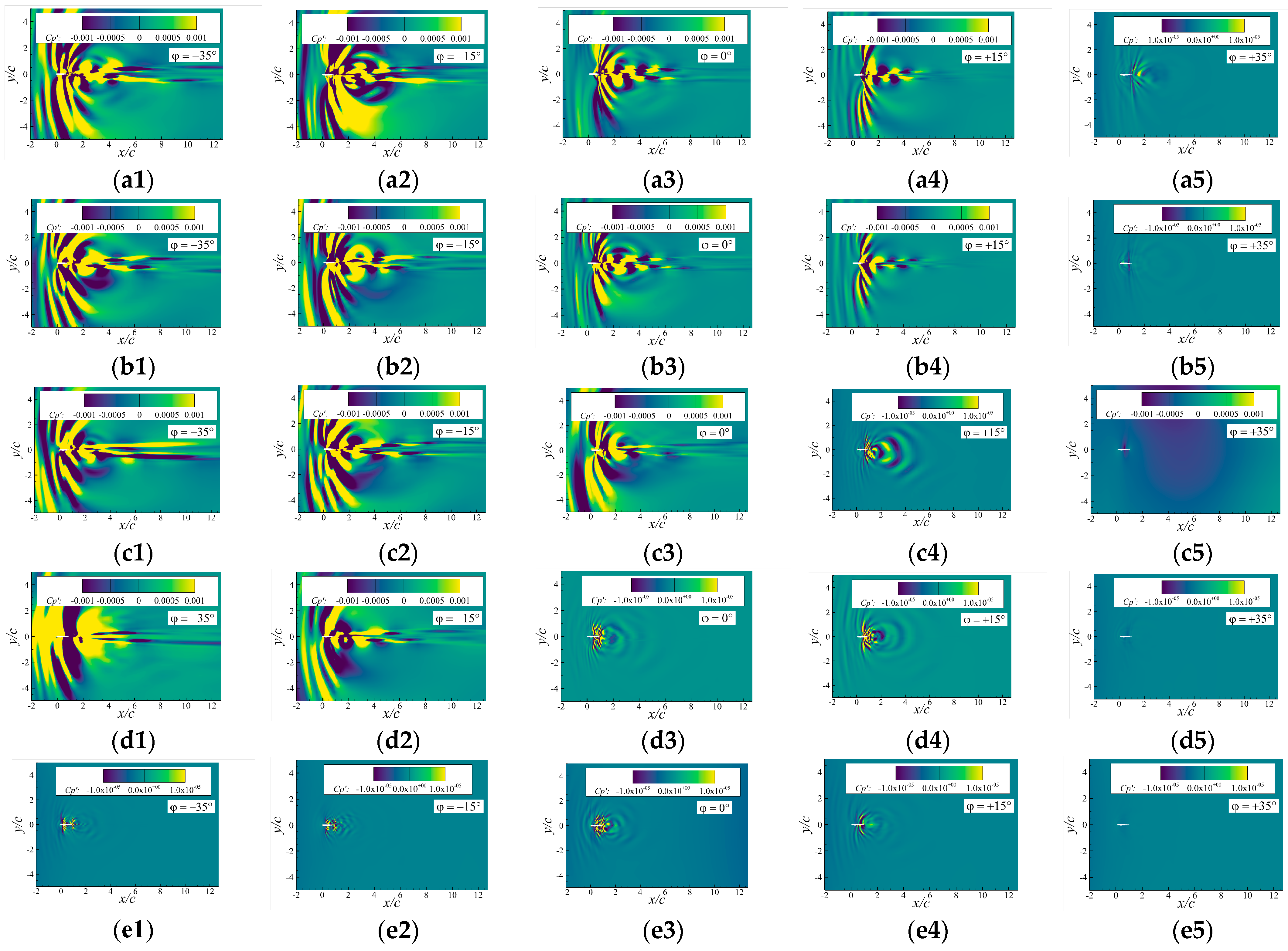
• When shock wave motion and boundary layer separation occur at the junction, pressure waves propagate to the side and upstream, while pressure waves propagate downstream due to vortex shedding on the bottom. When the flow at the junction is stable, turbulence occurs downstream of the entire span for the straight airfoil, in the root area for the forward-swept airfoil, and at the tip for the backward-swept airfoil.
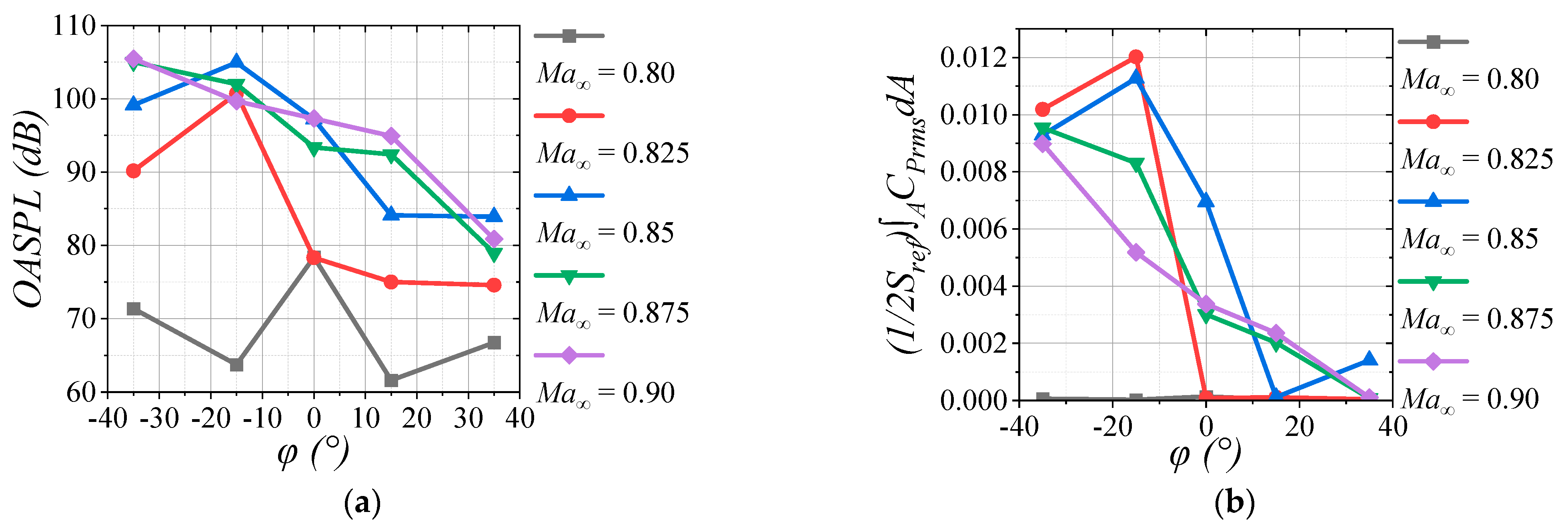
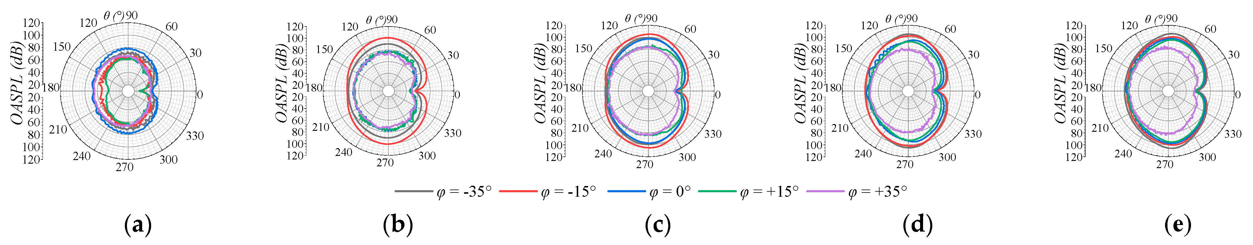
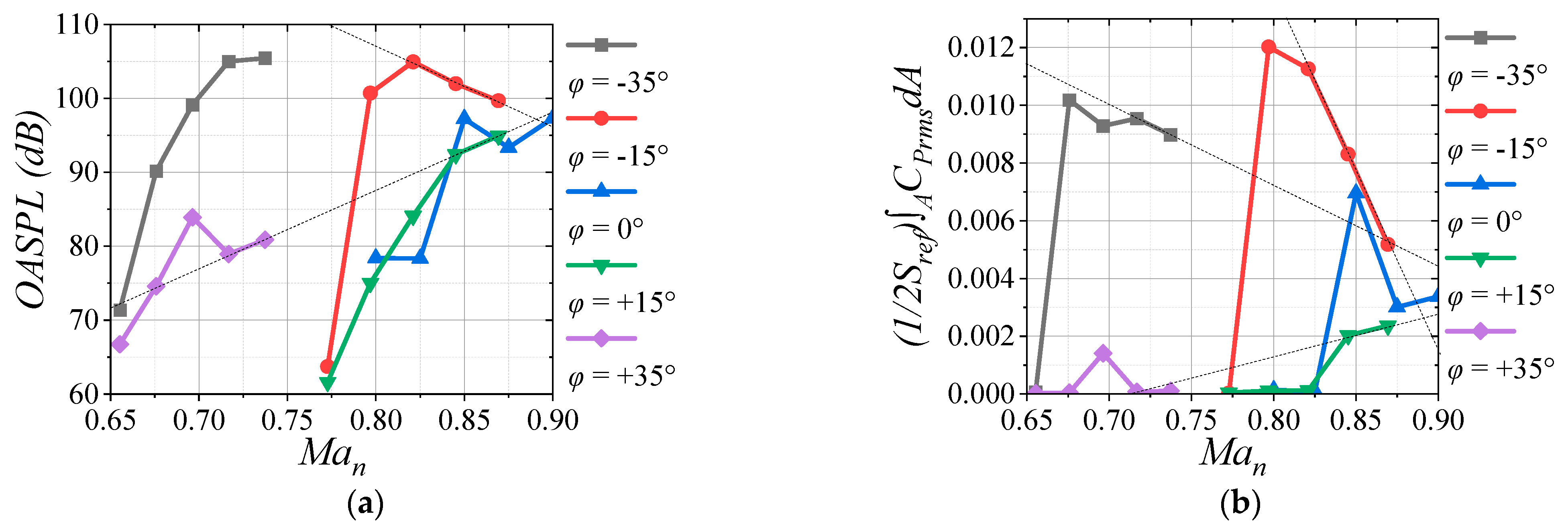
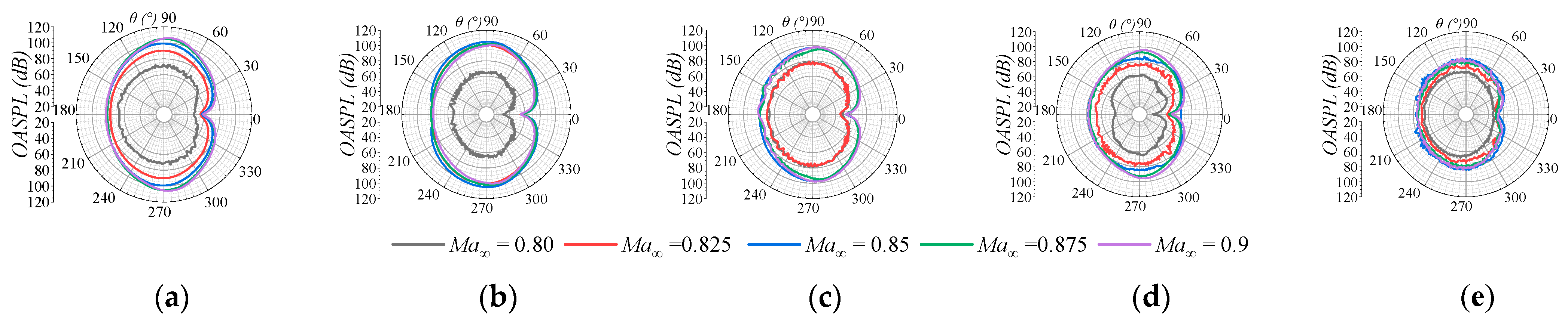
• The pressure fluctuation on the airfoil surface is the primary source of far-field noise generated by a wall-mounted finite-span airfoil in transonic conditions. The far-field directivity of this noise exhibits obvious dipole noise characteristics, and the curve is very smooth. In addition, the amplitude of far-field noise is positively correlated with normal Mach number and the absolute values of sweep angle.

In the context of attachments on the surface of an aircraft’s fuselage, the blade antennas, typically featuring a backward-swept design, generally do not exhibit significant vibration or noise issues, while for a pitot tube with a forward-swept strut, this study emphasizes the significance of addressing issues related to unsteady flow and far-field noise that may occur with an increase in the Mach number. Further research is needed on the issue of the probe noise of pitot tubes in transonic flow and the impact of probe and strut interaction. This may explain why pitot tube struts are generally not designed to sweep back to avoid SWBLIs at the junction. Due to the numerous cases considered in this study, a relatively coarse turbulence simulation method and a limited grid resolution are employed. The investigation of the change process of the flow field within a single shock wave motion period and the correlation between a specific frequency of noise and the flow field of each case remains unexplored. This paper does not discuss the shape and thickness of the boundary layer or the influence of the curvature of the bottom surface on the observed phenomena. These variables are pertinent to the actual fuselage surface, and the attachment installation site might encounter different boundary layer conditions and fuselage curvature. Investigating these elements could present potential avenues for further research.

References

1. Hu, N.; Buchholz, H.; Herr, M. Contributions of different aeroacoustic sources to aircraft cabin noise. In Proceedings of the 19th AIAA/CEAS Aeroacoustics Conference, Berlin, Germany, 27–29 May 2013. [Google Scholar] [CrossRef]
2. Havrilesko, B.R.; Hassan, M.; Denney, R.K.; Taiw, J.C. En route jet aircraft noise analysis. In Proceedings of the AIAA/3AF Aircraft Noise and Emissions Reduction Symposium, Atlanta, GA, USA, 16–20 June 2014. [Google Scholar] [CrossRef]
3. Moshkov, P. Contributions of different sources to cabin noise of a superjet 100 in cruise flight condition. In Proceedings of the AIAA AVIATION 2021 FORUM, Virtual Event, 2–6 August 2021. [Google Scholar] [CrossRef]
4. Mehta, R. Effect of wing nose shape on the flow in a wing body junction. Aeronaut. J. 1984, 88, 456. [Google Scholar] [CrossRef]
5. Simpson, R.L. Junction flows. Annu. Rev. Fluid Mech. 2001, 33, 415–443. [Google Scholar] [CrossRef]
6. Giuni, M.; Green, R.B. Vortex formation on squared and rounded tip. Aerosp. Sci. Technol. 2013, 29, 191–199. [Google Scholar] [CrossRef]
7. Karakus, C.; Akilli, H.; Sahin, B. Formation, structure, and development of the near-field wing tip vortices. Proc. Inst. Mech. Eng. Part G-J. Aerosp. Eng. 2008, 222, 13–22. [Google Scholar] [CrossRef]
8. Moreau, D.J.; Brooks, L.A.; Doolan, C.J. Broadband trailing edge noise from a sharp-edged strut. J. Acoust. Soc. Am. 2011, 129, 2820–2829. [Google Scholar] [CrossRef]
9. Arbey, H.; Bataille, J. Noise generated by airfoil profiles placed in a uniform laminar flow. J. Fluid Mech. 1983, 134, 33–47. [Google Scholar] [CrossRef]
10. Moreau, D.J.; Prime, Z.; Porteous, R.; Doolan, C.J.; Valeau, V. Flow-induced noise of a wall-mounted finite airfoil at low-to-moderate Reynolds number. J. Sound Vib. 2014, 333, 6924–6941. [Google Scholar] [CrossRef]
11. Moreau, D.J.; Doolan, C.J. Tonal noise production from a wall-mounted finite airfoil. J. Sound Vib. 2016, 363, 199–224. [Google Scholar] [CrossRef]
12. Brooks, T.F.; Hodgson, T.H. Trailing edge noise prediction from measured surface pressures. J. Sound Vib. 1981, 78, 69–117. [Google Scholar] [CrossRef]
13. Nash, E.C.; Lowson, M.V.; McAlpine, A. Boundary-layer instability noise on aerofoils. J. Fluid Mech. 1999, 382, 27–61. [Google Scholar] [CrossRef]
14. McAlpine, A.; Nash, E.C.; Lowson, M.V. On the generation of discrete frequency tones by the flow around an aerofoil. J. Sound Vib. 1999, 222, 753–779. [Google Scholar] [CrossRef]
15. Moreau, D.J.; Doolan, C.J. An Investigation of the Tonal Noise Produced by a Wall-Mounted Finite Airfoil at Angle of Attack, 22nd ed.; AIAA, Ed.; AIAA/CEAS: Lyon, France, 2016. [Google Scholar] [CrossRef]
16. Geyer, T.F.; Moreau, D.J. A study of the effect of airfoil thickness on the tonal noise generation of finite, wall-mounted airfoils. Aerosp. Sci. Technol. 2021, 115, 106768. [Google Scholar] [CrossRef]
17. Moreau, D.J.; Geyer, T.F.; Doolan, C.J.; Sarradj, E. Camber effects on the tonal noise and flow characteristics of a wall-mounted finite airfoil. In Proceedings of the 23rd AIAA/CEAS Aeroacoustics Conference, Denver, Colorado, 5–9 June 2017; pp. 2017–3172. [Google Scholar] [CrossRef]
18. Moreau, D.J.; Geyer, T.F.; Doolan, C.J.; Sarradj, E. Surface curvature effects on the tonal noise of a wall-mounted finite airfoil. J. Acoust. Soc. Am. 2018, 143, 3460–3473. [Google Scholar] [CrossRef]
19. Zhang, T.; Geyer, T.F.; Silva, C.; Fischer, J.R.; Doolan, C.J.; Moreau, D.J. Experimental investigation of tip vortex formation noise produced by wall-mounted finite airfoils. J. Aerosp. Eng. 2021, 34, 4021079. [Google Scholar] [CrossRef]
20. Giez, J.; Vion, L.; Roger, M.; Moreau, S. Effect of the edge and tip vortex on airfoil self-noise and Turbulence Impingement Noise. In Proceedings of the 22nd AIAA/CEAS Aeroacoustics Conference, Lyon, France, 30 May–1 June 2016; AIAA Paper. pp. 2016–2996. [Google Scholar] [CrossRef]
21. Yakhina, G.R.; Roger, M.; Finez, A.; Bouley, S.; Baron, V.; Moreau, S.; Giez, J. Localization of swept free-tip airfoil noise sources by microphone array processing. AIAA J. 2020, 58, 3414–3425. [Google Scholar] [CrossRef]
22. Grasso, G.; Roger, M.; Moreau, S. Effect of sweep angle and of wall-pressure statistics on the free-field directivity of airfoil trailing-edge noise. In Proceedings of the 25th AIAA/CEAS Aeroacoustics Conference, Delft, The Netherlands, 20–23 May 2019; AIAA Paper. pp. 2019–2612. [Google Scholar] [CrossRef]
23. Grasso, G.; Roger, M.; Moreau, S. Analytical model of the source and radiation of sound from the trailing edge of a swept airfoil. J. Sound Vib. 2021, 493, 115838. [Google Scholar] [CrossRef]
24. Koch, R.; Sanjosé, M.; Moreau, S. Acoustic investigation of the transonic RAE 2822 airfoil with large-eddy simulation. In Proceedings of the 28th AIAA/CEAS Aeroacoustics Conference, Southampton, UK, 14–17 June 2022; AIAA Paper. pp. 2022–2816. [Google Scholar] [CrossRef]
25. Alguacil, A.; Becherucci, L.; Sanjosé, M.; Moreau, S. Broadband noise of the transonic RAE 2822 Airfoil. In Proceedings of the AIAA AVIATION Forum, San Diego, CA, USA, 12–16 June 2023; AIAA Paper. pp. 2023–3635. [Google Scholar] [CrossRef]
26. Zhang, Q.; Gao, C.; Zhou, F.; Yang, D.; Zhang, W. Study on flow noise characteristic of transonic deep buffeting over an airfoil. Phys. Fluids 2023, 35, 046109. [Google Scholar] [CrossRef]
27. Zhong, S.Y.; Zhang, X.; Gill, J.; Fattah, R.; Sun, Y.H. A numerical investigation of the airfoil-gust interaction noise in transonic flows: Acoustic processes. J. Sound Vib. 2018, 425, 239–256. [Google Scholar] [CrossRef]
28. Zhong, S.Y.; Zhang, X.; Gill, J.; Fattah, R.; Sun, Y.H. Geometry effect on the airfoil-gust interaction noise in transonic flows. Aerosp. Sci. Technol. 2019, 92, 181–191. [Google Scholar] [CrossRef]
29. Ruban, A.I.; Bernots, T.; Kravtsova, M.A. Linear and nonlinear receptivity of the boundary layer in transonic flows. J. Fluid Mech. 2016, 786, 154–189. [Google Scholar] [CrossRef]
30. Wang, Y.; Xu, J.; Qiao, L.; Zhang, Y.; Junqiang Bai, J. Improved Amplification Factor Transport Transition Model for Transonic Boundary Layers. AIAA J. 2023, 61, 2022–4030. [Google Scholar] [CrossRef]
31. Clemens, N.T.; Narayanaswamy, V. Low-frequency unsteadiness of shock wave/turbulent boundary layer interactions. Annu. Rev. Fluid Mech. 2014, 46, 469–492. [Google Scholar] [CrossRef]
32. Gaitonde, D.V. Progress in shock wave/boundary layer interactions. Prog. Aeosp. Sci. 2015, 72, 80–99. [Google Scholar] [CrossRef]
33. Gaitonde, D.V.; Adler, M.C. Dynamics of three-dimensional shock-wave/boundary-layer interactions. Annu. Rev. Fluid Mech. 2023, 55, 291–321. [Google Scholar] [CrossRef]
34. Tô, J.B.; Simiriotis, N.; Marouf, A.; Szubert, D.; Asproulias, I.; Zilli, D.M.; Hoarau, Y.; Hunt, J.C.R.; Braza, M. Effects of vibrating and deformed trailing edge of a morphing supercritical airfoil in transonic regime by numerical simulation at high Reynolds number. J. Fluids Struct. 2019, 91, 102595. [Google Scholar] [CrossRef]
35. Szulc, O.; Doerffer, P.; Flaszynski, P.; Suresh, T. Numerical modelling of shock wave-boundary layer interaction control by passive wall ventilation. Comput. Fluids 2020, 200, 104435. [Google Scholar] [CrossRef]
36. Poplingher, L.; Raveh, D.E. Comparative Modal Study of the Two-Dimensional and Three-Dimensional Transonic Shock Buffet. AIAA J. 2023, 61, 2022–2483. [Google Scholar] [CrossRef]
37. D’Aguanno, A.; Schrijer, F.F.J.; Oudheusden, B.W. Finite-Wing and Sweep Effects on Transonic Buffet Behavior. AIAA J. 2022, 60, 6715–6725. [Google Scholar] [CrossRef]
38. Gleize, V.; Dumont, A.; Mayeur, J.; Destarac, D. RANS simulations on TMR test cases and M6 wing with the Onera elsA flow solver. Turbulent Flow. In Proceedings of the Solutions for NACA 0012 and Other Test Cases from the Turbulence Model Resource Website: Residual and Grid Convergence II, Kissimmee, FL, USA, 5–9 January 2015; AIAA Paper. pp. 1745–2015. [Google Scholar] [CrossRef]
39. Mayeur, J.; Dumont, A.; Gleize, V.; Destarac, D. RANS simulations on TMR 3D test cases with the Onera elsA flow solver. In Proceedings of the Special Session: Evaluation of RANS Solvers on Benchmark Aerodynamic Flows II, San Diego, CA, USA, 4–8 January 2016; AIAA Paper. pp. 1357–2016. [Google Scholar] [CrossRef]
Figure 1. Fuselage attachments on large commercial airliner: (a) blade antennas; (b) pitot tubes.
Aerospace 11 00645 g001
Figure 2. Wall-mounted finite-span wing model and calculation grid ( φ = +35°, for example).
Aerospace 11 00645 g002
Figure 3. The positions of the far-field noise measurement point. The directivity is taken from the circumference.
Aerospace 11 00645 g003
Figure 4. Velocity and turbulent kinetic energy profile near bottom wall at P1 ( x / c = −0.1, y / c = 0) and P2 ( x / c = 0, y / c = 1) of the result of the straight airfoil at M a = 0.85.
Aerospace 11 00645 g004
Figure 5. Comparison between numerical simulation and theoretical solution of boundary layer at ( x / c = −0.1, y / c = 0) and P2 ( x / c = 0, y / c = 1).
Aerospace 11 00645 g005
Figure 6. Validation of numerical simulation by comparing with experimental results of ONERA M6 wing Case 2308: (a) z / b = 0.2; (b) z / b = 0.44; (c) z / b = 0.65; (d) z / b = 0.8. b is the wing span.
Aerospace 11 00645 g006
Figure 7. The surface streamline, pressure coefficient, and shock position ( U a · p p = 16 ): (a1) φ = −35°, M a = 0.90; (a2) φ = −15°, M a = 0.90; (a3) φ = 0°, M a = 0.90; (a4) φ = +15°, M a = 0.90; (a5) φ = +35°, M a = 0.90; (b1) φ = −35°, M a = 0.875; (b2) φ = −15°, M a = 0.875; (b3) φ = 0°, M a = 0.875; (b4) φ = +15°, M a = 0.875; (b5) φ = +35°, M a = 0.875; (c1) φ = −35°, M a = 0.85; (c2) φ = −15°, M a = 0.85; (c3) φ = 0°, M a = 0.85; (c4) φ = +15°, M a = 0.85; (c5) φ = +35°, M a = 0.85; (d1) φ = −35°, M a = 0.825; (d2) φ = −15°, M a = 0.825; (d3) φ = 0°, M a = 0.825; (d4) φ = +15°, M a = 0.825; (d5) φ = +35°, M a = 0.825; (e1) φ = −35°, M a = 0.80; (e2) φ = −15°, M a = 0.80; (e3) φ = 0°, M a = 0.80; (e4) φ = +15°, M a = 0.80; (e5) φ = +35°, M a = 0.80.
Aerospace 11 00645 g007aAerospace 11 00645 g007b
Figure 8. The root-mean-square surface pressure coefficient: (a1) φ = −35°, M a = 0.90; (a2) φ = −15°, M a = 0.90; (a3) φ = 0°, M a = 0.90; (a4) φ = +15°, M a = 0.90; (a5) φ = +35°, M a = 0.90; (b1) φ = −35°, M a = 0.875; (b2) φ = −15°, M a = 0.875; (b3) φ = 0°, M a = 0.875; (b4) φ = +15°, M a = 0.875; (b5) φ = +35°, M a = 0.875; (c1) φ = −35°, M a = 0.85; (c2) φ = −15°, M a = 0.85; (c3) φ = 0°, M a = 0.85; (c4) φ = +15°, M a = 0.85; (c5) φ = +35°, M a = 0.85; (d1) φ = −35°, M a = 0.825; (d2) φ = −15°, M a = 0.825; (d3) φ = 0°, M a = 0.825; (d4) φ = +15°, M a = 0.825; (d5) φ = +35°, M a = 0.825; (e1) φ = −35°, M a = 0.80; (e2) φ = −15°, M a = 0.80; (e3) φ = 0°, M a = 0.80; (e4) φ = +15°, M a = 0.80; (e5) φ = +35°, M a = 0.80.
Aerospace 11 00645 g008
Figure 9. The iso-surface colored by the time-averaged pressure coefficient of k = 10   m 2/s2 and the streamlines in the junction areas of cases with obvious junction separation. The purple surface represents the shock position, as illustrated in Figure 7: (a1) φ = −35°, M a = 0.90; (a2) φ = −15°, M a = 0.90; (a3) φ = 0°, M a = 0.90; (a4) φ = +15°, M a = 0.90; (b1) φ = −35°, M a = 0.875; (b2) φ = −15°, M a = 0.875; (b3) φ = 0°, M a = 0.875; (b4) φ = +15°, M a = 0.875; (c1) φ = −35°, M a = 0.85; (c2) φ = −15°, M a = 0.85; (c3) φ = 0°, M a = 0.85; (c4) φ = +15°, M a = 0.85.
Aerospace 11 00645 g009aAerospace 11 00645 g009b
Figure 10. Normalized root mean square of velocity u r m s / u in the plane y / c = −0.1. The isograms of the time-averaged Mach number are marked in the figure as follows: (a1) φ = −35°, M a = 0.90; (a2) φ = −15°, M a = 0.90; (a3) φ = 0°, M a = 0.90; (a4) φ = +15°, M a = 0.90; (b1) φ = −35°, M a = 0.875; (b2) φ = −15°, M a = 0.875; (b3) φ = 0°, M a = 0.875; (b4) φ = +15°, M a = 0.875; (c1) φ = −35°, M a = 0.85; (c2) φ = −15°, M a = 0.85; (c3) φ = 0°, M a = 0.85; (c4) φ = +15°, M a = 0.85.
Aerospace 11 00645 g010aAerospace 11 00645 g010b
Figure 11. Reynolds shear stress u v ¯ / u 2 in the plane y / c = −0.1. The isograms of the time-averaged Mach number are marked in the figure as follows: (a1) φ = −35°, M a = 0.90; (a2) φ = −15°, M a = 0.90; (a3) φ = 0°, M a = 0.90; (a4) φ = +15°, M a = 0.90; (b1) φ = −35°, M a = 0.875; (b2) φ = −15°, M a = 0.875; (b3) φ = 0°, M a = 0.875; (b4) φ = +15°, M a = 0.875; (c1) φ = −35°, M a = 0.85; (c2) φ = −15°, M a = 0.85; (c3) φ = 0°, M a = 0.85; (c4) φ = +15°, M a = 0.85.
Aerospace 11 00645 g011
Figure 12. Reynolds shear stress u w ¯ / u 2 in the plane y / c = −0.1. The isograms of the time-averaged Mach number are marked in the figure as follows: (a1) φ = −35°, M a = 0.90; (a2) φ = −15°, M a = 0.90; (a3) φ = 0°, M a = 0.90; (a4) φ = +15°, M a = 0.90; (b1) φ = −35°, M a = 0.875; (b2) φ = −15°, M a = 0.875; (b3) φ = 0°, M a = 0.875; (b4) φ = +15°, M a = 0.875; (c1) φ = −35°, M a = 0.85; (c2) φ = −15°, M a = 0.85; (c3) φ = 0°, M a = 0.85; (c4) φ = +15°, M a = 0.85.
Aerospace 11 00645 g012aAerospace 11 00645 g012b
Figure 13. Reynolds shear stress v w ¯ / u 2 in the plane y / c = −0.1. The isograms of the time-averaged Mach number are marked in the figure as follows: (a1) φ = −35°, M a = 0.90; (a2) φ = −15°, M a = 0.90; (a3) φ = 0°, M a = 0.90; (a4) φ = +15°, M a = 0.90; (b1) φ = −35°, M a = 0.875; (b2) φ = −15°, M a = 0.875; (b3) φ = 0°, M a = 0.875; (b4) φ = +15°, M a = 0.875; (c1) φ = −35°, M a = 0.85; (c2) φ = −15°, M a = 0.85; (c3) φ = 0°, M a = 0.85; (c4) φ = +15°, M a = 0.85.
Aerospace 11 00645 g013
Figure 14. Instantaneous pressure coefficient fluctuation ( C P ) near the bottom surface ( z / c = 0.1): (a1) φ = −35°, M a = 0.90; (a2) φ = −15°, M a = 0.90; (a3) φ = 0°, M a = 0.90; (a4) φ = +15°, M a = 0.90; (a5) φ = +35°, M a = 0.90; (b1) φ = −35°, M a = 0.875; (b2) φ = −15°, M a = 0.875; (b3) φ = 0°, M a = 0.875; (b4) φ = +15°, M a = 0.875; (b5) φ = +35°, M a = 0.875; (c1) φ = −35°, M a = 0.85; (c2) φ = −15°, M a = 0.85; (c3) φ = 0°, M a = 0.85; (c4) φ = +15°, M a = 0.85; (c5) φ = +35°, M a = 0.85; (d1) φ = −35°, M a = 0.825; (d2) φ = −15°, M a = 0.825; (d3) φ = 0°, M a = 0.825; (d4) φ = +15°, M a = 0.825; (d5) φ = +35°, M a = 0.825; (e1) φ = −35°, M a = 0.80; (e2) φ = −15°, M a = 0.80; (e3) φ = 0°, M a = 0.80; (e4) φ = +15°, M a = 0.80; (e5) φ = +35°, M a = 0.80.
Aerospace 11 00645 g014
Figure 15. Instantaneous pressure coefficient fluctuation ( C P ) in y / c = 0 slice: (a1) φ = −35°, M a = 0.90; (a2) φ = −15°, M a = 0.90; (a3) φ = 0°, M a = 0.90; (a4) φ = +15°, M a = 0.90; (a5) φ = +35°, M a = 0.90; (b1) φ = −35°, M a = 0.875; (b2) φ = −15°, M a = 0.875; (b3) φ = 0°, M a = 0.875; (b4) φ = +15°, M a = 0.875; (b5) φ = +35°, M a = 0.875; (c1) φ = −35°, M a = 0.85; (c2) φ = −15°, M a = 0.85; (c3) φ = 0°, M a = 0.85; (c4) φ = +15°, M a = 0.85; (c5) φ = +35°, M a = 0.85; (d1) φ = −35°, M a = 0.825; (d2) φ = −15°, M a = 0.825; (d3) φ = 0°, M a = 0.825; (d4) φ = +15°, M a = 0.825; (d5) φ = +35°, M a = 0.825; (e1) φ = −35°, M a = 0.80; (e2) φ = −15°, M a = 0.80; (e3) φ = 0°, M a = 0.80; (e4) φ = +15°, M a = 0.80; (e5) φ = +35°, M a = 0.80.
Aerospace 11 00645 g015
Figure 16. Instantaneous pressure coefficient fluctuation ( C P ) in x / c = 0.025 slice: (a1) φ = −35°, M a = 0.90; (a2) φ = −15°, M a = 0.90; (a3) φ = 0°, M a = 0.90; (a4) φ = +15°, M a = 0.90; (a5) φ = +35°, M a = 0.90; (b1) φ = −35°, M a = 0.875; (b2) φ = −15°, M a = 0.875; (b3) φ = 0°, M a = 0.875; (b4) φ = +15°, M a = 0.875; (b5) φ = +35°, M a = 0.875; (c1) φ = −35°, M a = 0.85; (c2) φ = −15°, M a = 0.85; (c3) φ = 0°, M a = 0.85; (c4) φ = +15°, M a = 0.85; (c5) φ = +35°, M a = 0.85; (d1) φ = −35°, M a = 0.825; (d2) φ = −15°, M a = 0.825; (d3) φ = 0°, M a = 0.825; (d4) φ = +15°, M a = 0.825; (d5) φ = +35°, M a = 0.825; (e1) φ = −35°, M a = 0.80; (e2) φ = −15°, M a = 0.80; (e3) φ = 0°, M a = 0.80; (e4) φ = +15°, M a = 0.80; (e5) φ = +35°, M a = 0.80.
Aerospace 11 00645 g016
Figure 17. Comparison between (a) OASPL at the direction of θ = 90° and (b) normalized integral C P r m s on airfoil surface for each M a .
Aerospace 11 00645 g017
Figure 18. Far-field noise directivities of airfoils with every φ for each M a : (a) M a = 0.80; (b) M a = 0.825; (c) M a = 0.85; (d) M a = 0.875; (e) M a = 0.90.
Aerospace 11 00645 g018
Figure 19. Comparison between (a) OASPL at the direction of θ = 90° and (b) normalized integral C P r m s on airfoil surface for each φ .
Aerospace 11 00645 g019
Figure 20. Far-field directivities at every M a for airfoils with every φ : (a) φ = −35°; (b) φ = −15°; (c) φ = 0°; (d) φ = +15°; (e) φ = +35°.
Aerospace 11 00645 g020