Abstract
Data mining has achieved great success in air traffic management as a technology for learning knowledge from historical data that benefits people. However, data mining can rarely be embedded into the trajectory optimization process since regular optimization algorithms cannot utilize the functional and implicit knowledge extracted from historical data in a general paradigm. To tackle this issue, this research proposes a novel data mining-based trajectory generation method that is compatible with existing optimization algorithms. Firstly, the proposed method generates trajectories by combining various maneuvers learned from operation data instead of reconstructing trajectories with generative models. In such a manner, data mining-based trajectory optimization can be achieved by solving a combinatorial optimization problem. Secondly, the proposed method introduces a majorization–minimization-based adversarial training paradigm to train the generation model with more general loss functions, including non-differentiable flight performance constraints. A case study on Guangzhou Baiyun International Airport was conducted to validate the proposed method. The results illustrate that the trajectory generation model can generate trajectories with high fidelity, diversity, and flyability.
1. Introduction
1.1. Motivation
Society has entered a data-driven era in which huge amounts of data are being generated every day. In the last decade, more and more researchers have focused on mining useful information from historical data to create benefits for people. Accordingly, various data-based applications have been developed, including traffic-related mining [1,2], autonomous path planning [3,4,5], and popular route discovery [6]. In the air traffic management domain, trajectory data have been used to identify traffic patterns [7,8,9], estimate the loss of separation probability [10], and gain operation experience [11,12].
However, the knowledge learned from historical data can rarely be utilized in optimization since it belongs to functional space. To tackle this issue, this paper proposes a novel trajectory generation method embedded with data mining that can be compatible with optimization algorithms. Compared with the other data-driven trajectory generation methods mentioned in Section 1.2, the proposed method can automatically mine helpful information (all kinds of pilot maneuvers) from historical data to improve generation performance.
1.2. Related Work
This study defines three requirements that the trajectory generation method should meet: firstly, fidelity—synthetic trajectories should follow the characteristics of actual trajectories [13]; secondly, diversity—the proposed method could reproduce some trajectories with a small probability of occurrence; and thirdly, flyability—synthetic trajectories should meet the flight performance constraints.
The current research on trajectory generation can be divided into model-driven and data-driven methods. Model-driven methods [14,15] generate aircraft trajectories based on kinetic and kinematic models with several parameters, such as initial aircraft states, aircraft performance coefficients [16,17], weather conditions, and aircraft intents. Since these methods depend on the model and parameters of aircraft, the trajectories generated by these models can undoubtedly meet the requirement of flyability. To ensure the generation of trajectories with good diversity, some model-driven methods [18,19,20] adopt the free-flight concept [21,22] and do not fly along the published flight routes. However, such an approach induces poor fidelity of trajectories since they have different distributions from the actual ones. To address the poor-fidelity problem, other model-driven methods [23,24,25,26] search for optimal flight paths among predefined routes, such as Standard Terminal Arrival Routes and some of their related deviation patterns. However, due to the commonly existing long-tail effect, these predefined routes are limited and not enough to describe all the potential routes in real operation, leading to the homogenization of generated trajectories (poor diversity).
Incorporating controllers’ experience from historical data while generating trajectories can be a promising approach to improve fidelity and diversity. Data-driven methods have been intensively explored to generate trajectories using machine learning algorithms in the ground transportation field [27,28,29,30,31]. Some trajectory generation models have exploited Multilayer Perceptron [32], Long Short-Term Memory (LSTM) [33], and convolutional neural networks [34] to extract spatial–temporal features from actual trajectories. Other trajectory generation models have taken advantage of Variational Auto-Encoders (VAEs) [35], Generative Adversarial Networks [36], and their variants (GANs) [37,38] to create new trajectories. With the success of data-driven data generation in ground transportation, several researchers have extended this concept to generate aircraft trajectories with data-driven methods. Existing solutions include VampPrior TCVAE [39], Conv1D-GAN [40], Gaussian mixture model-based generators [41], Principal Component Analysis (PCA) [42], and functional PCA [43].
However, existing data-driven trajectory generation methods have the following drawbacks:
- For most trajectory generation models, one cannot tell what a generated trajectory looks like before obtaining the final results. To tackle this issue, Ref. [43] generated trajectories via functional PCA and controlled the shape of the trajectories by modifying the mean and principal component functions. Analogously, Krauth et al. [39] controlled the shape of trajectories by sampling points in certain areas in latent space. Although these efforts partially solved the problem and enable one to roughly determine the shape of trajectories, uncertainties still remain in the generation process. Thus, these data-driven methods can rarely cooperate with optimization algorithms to generate optimal trajectories.
- Existing methods prefer to exploit a distribution to capture the flight path deviations. However, deviations are not only caused by uncertainties such as weather, aircraft performance, and human factors, but are also caused by controllers’ instructions. Unlike uncertainties in actual operations, the controller’s instructions must always meet certain rules and cannot be modeled through a distribution. To imitate controllers’ instructions, Jarry et al. [43] additionally introduced several modification operators to change the shape of trajectories. However, such a method requires some fine-tuning by experts and cannot automatically learn controllers’ experience (instructions).
- Existing data-driven generation models can only be trained with differentiable loss functions, whereas flight performance constraints are often non-differentiable. Thus, the generated trajectories may not be able to stay flyable. The key to solving this problem is to build a neural network with more general loss functions. To this end, some researchers have adopted a strategy that approximates non-differentiable constraints with differentiable functions [44,45,46,47,48,49].
To overcome all the issues mentioned above, this paper develops a novel data-driven method called CTG-MMAT to generate trajectories. Firstly, a connection-based trajectory generation (CTG) framework is proposed to automatically mine helpful information (all kinds of maneuvers) from historical trajectories. Secondly, a majorization–minimization-based adversarial training (MMAT) paradigm is adopted to train the trajectory generation model with flight performance constraints. The main contributions of this paper are summarized as follows:
- The proposed CTG-MMAT is compatible with combinatorial optimization algorithms to build a data-driven trajectory optimization methodology by combining several maneuvers.
- The proposed CTG framework enables the trajectory generation model to capture more controllers’ experiences from historical data. As a result, the generated trajectories are closer to the ones observed in the operations.
- The proposed MMAT technique enables the trajectory generation model to be trained with a more general loss function with non-differentiable flight performance constraints. As a result, the generated trajectories are more likely to stay flyable.
The remainder of this paper is organized as follows: Section 2 introduces the proposed CTG framework in detail and discusses why the proposed method has the potential to be used in trajectory optimization. Section 3 presents the MMAT, which is a non-differentiable constraint approximation technique. Section 4 provides details about the experiment. The results of Section 5 are divided into three parts. Section 5.1 analyzes the flyability of the generated trajectories by comparing CTG-MMAT with existing methods. Section 5.2 highlights how CTG-MMAT incorporates operation rules while generating trajectories. Section 5.3 highlights how CTG-MMAT generates trajectories with the controllers’ experience. Section 5.4 demonstrates how the CTG framework reduces training costs while maintaining generation performance. Section 6 concludes this work and describes the direction for future research.
2. Connection-Based Trajectory Generation Framework
To fully utilize the controller’s experience while generating trajectories, this paper presents a novel trajectory generation framework. Compared with existing data-driven trajectory generation methods, the proposed framework generates a new trajectory by combining several maneuvers.
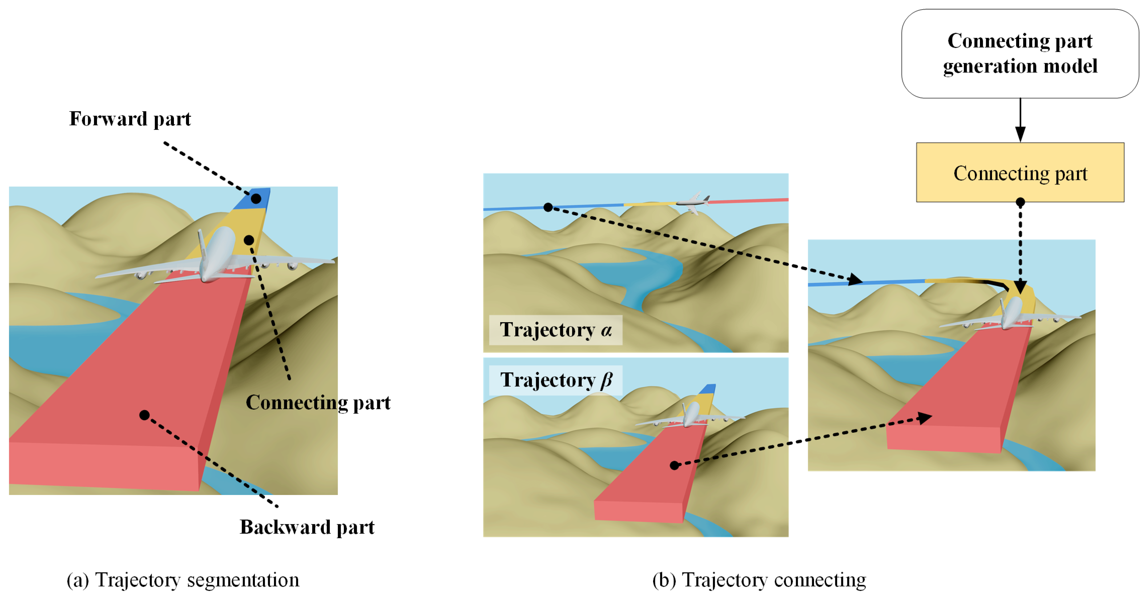
As shown in Figure 1, instead of generating a complete trajectory at a time, the proposed CTG generates a trajectory by connecting several sub-trajectories. Figure 1a shows the trajectory segmentation process: a complete trajectory is divided into backward, connecting, and forward parts. Figure 1b shows the trajectory connection process: given the forward part of trajectory and the backward part of trajectory , a connecting part is generated by a generation model to connect the backward and forward parts.
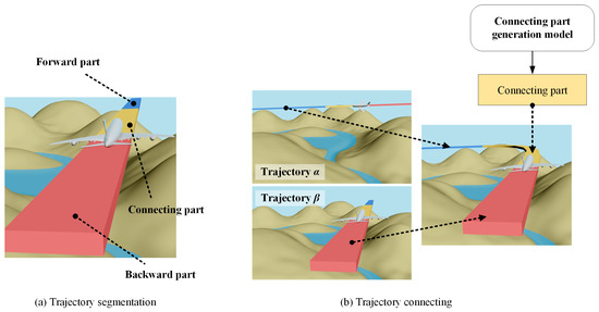
Figure 1.
Framework of the proposed CTG. Firstly, the complete trajectory is divided into backward, connecting, and forward parts; secondly, a new connecting part is generated to connect the backward and forward parts from different trajectories to obtain a new synthetic trajectory.
The key to achieving CTG is generating a proper connecting part for the forward and backward parts. To this end, this paper trains a connecting part generation model via supervised learning. The input data include the forward and backward parts, and the output data include the connecting part.
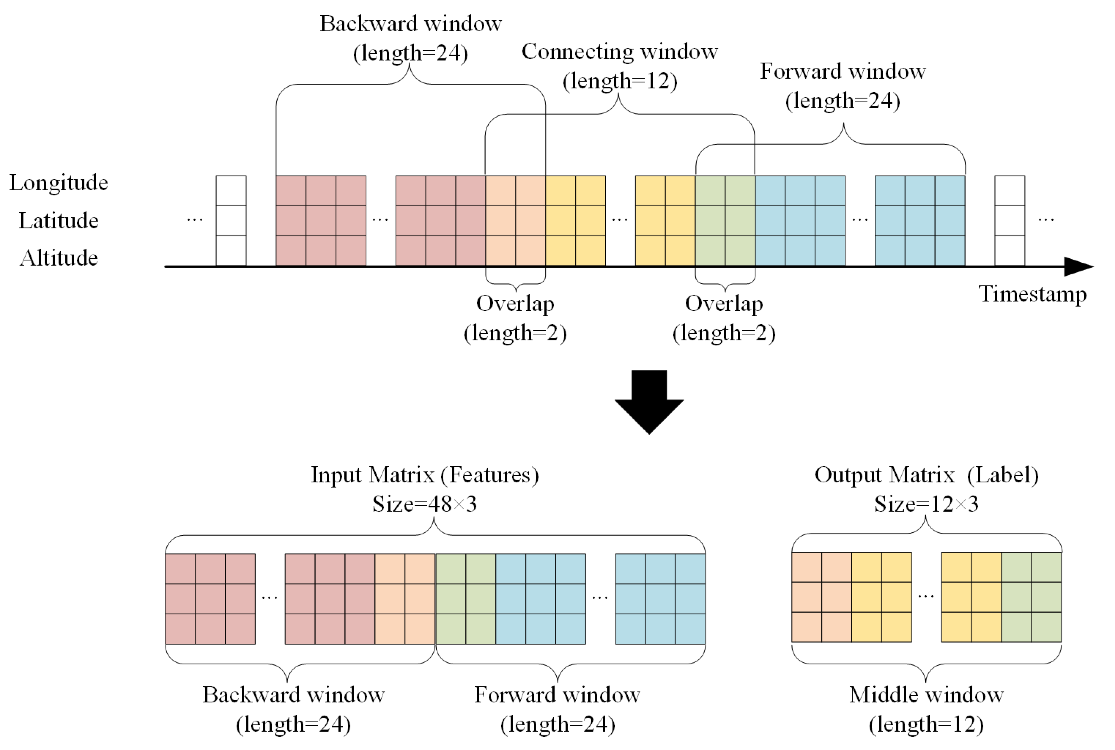
The training data preparation process is given in Figure 2. Firstly, the historical trajectories are resampled with equal time intervals. Each trajectory point includes latitude, longitude, and altitude information. The time interval is set to 10 s. Then, the resampled trajectories are normalized to make training more straightforward. Finally, the training data are collected through three sliding windows: backward, connecting, and forward windows. Among them, the backward and forward windows are used to obtain the features (input data) of the supervised generation model, and the connecting window is used to obtain labels (output data). According to the sensitivity analysis given in Appendix A, the length of these three windows should be set to 24, 12, and 24, respectively.
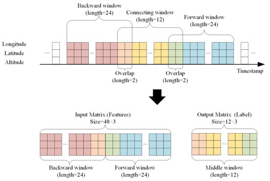
Figure 2.
Schematic diagram of training data preparation for connecting part generation model. Training data are collected by utilizing three partially overlapping sliding windows: the backward and forward windows, which are used to obtain input data, and the connecting window, which is used to obtain output data. The red, yellow, and blue boxes refer to the part of the backward, connecting, and forward windows that do not overlap with other windows, respectively. The orange and green boxes refer to the overlapping part of two adjacent windows.
According to Figure 2, both the features and labels for training the model are matrixes composed of several trajectory points. Each row of the matrix represents a timestamp, and each column represents a dimension of a 3D trajectory point. The size of a feature is , and the size of a label is .
This study intentionally introduces data leakage while collecting training data. As shown in Figure 2, the connecting window partially overlaps with the others. In such a manner, the overlapping parts simultaneously exist in the features and labels, and the supervised model can easily learn to generate a connecting part to connect the backward and forward parts seamlessly.
Since the proposed CTG takes the best advantage of the controller’s experience extracted from historical data, its benefits are obvious. On the one hand, the fidelity of the generated trajectories is high since most parts of a synthetic trajectory are from real ones. On the other hand, the diversity of the generated trajectories is high since the proposed framework enables us to modularize trajectories and create new ones by connecting sub-trajectories with various flight intentions.
Although the CTG framework can generate trajectories with high diversity and fidelity, it has a critical problem that needs to be solved before being applied. The problem is finding proper forward trajectories for a given backward trajectory to ensure the generated trajectories are flyable. On the one hand, if the backward and forward parts are far from each other, it is impossible to find a proper connecting part. On the other hand, even if the backward and forward parts are close enough, the CTG cannot guarantee that the generated connecting parts meet the flight performance constraints. To solve these problems, this paper employs majorization–minimization (MM) to add the non-differentiable flight performance constraints to the supervised generation model and propose a two-round flyable trajectory filtering mechanism to eliminate unfeasible trajectories. Section 3 describes this process in detail.
Compatibility with Optimization Algorithms
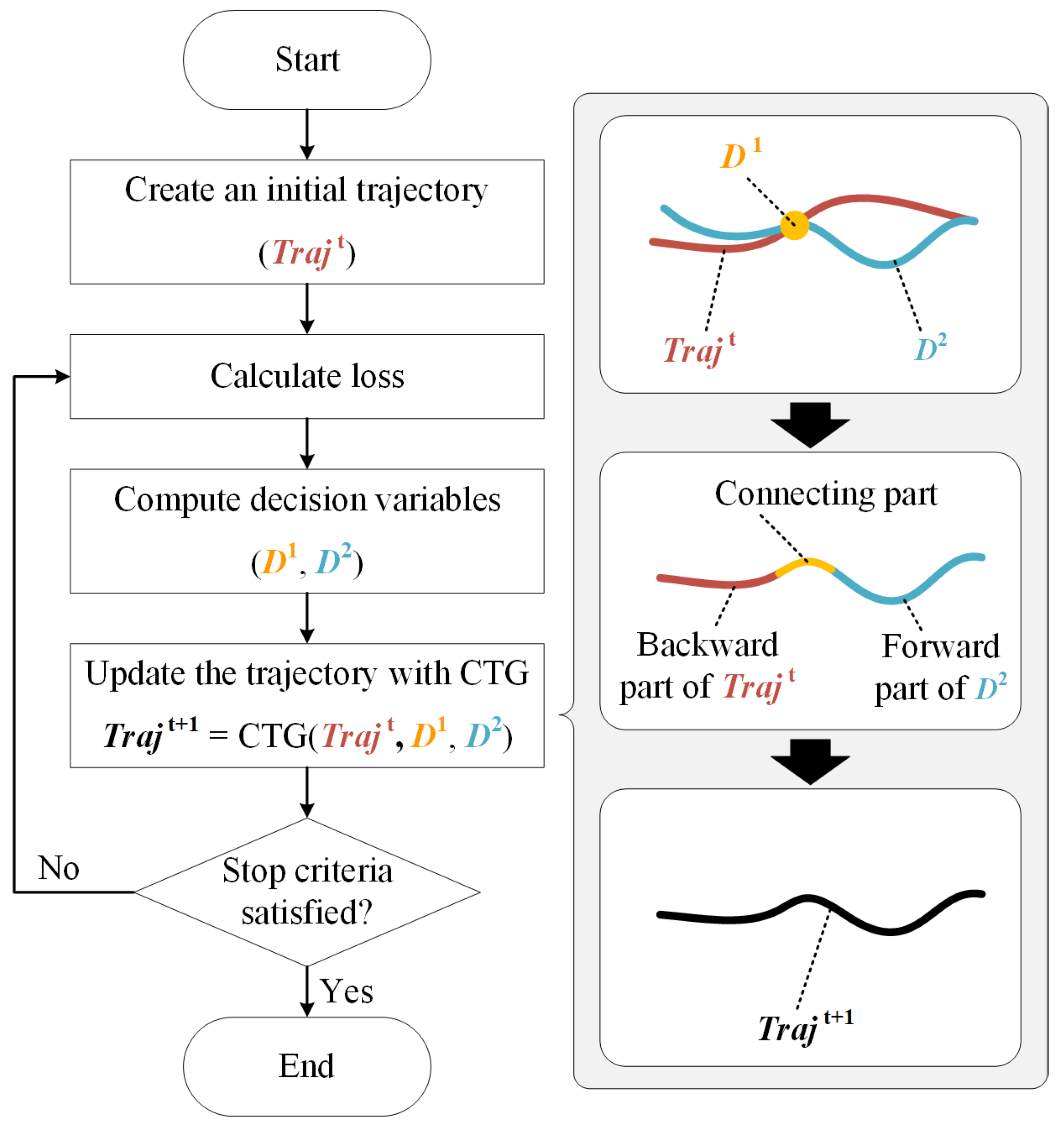
This is a short sub-section showing how the CTG could be used in an optimization loop. Considering that the proposed CTG provides an efficient way to modify a trajectory, it can be plugged into an optimization algorithm to achieve trajectory optimization in the future.
As shown in Figure 3, the CTG can be applied in an optimization loop to update the trajectory. Firstly, the loss of the original trajectory can be computed to represent the goodness of the current trajectory. Then, some optimization algorithms, such as genetic algorithms and simulated annealing, can be used to compute decision variables, which are used to update the original trajectory via the proposed CTG. Finally, if the stop criteria are satisfied, the optimized trajectory is obtained; otherwise, we proceed to the next iteration.
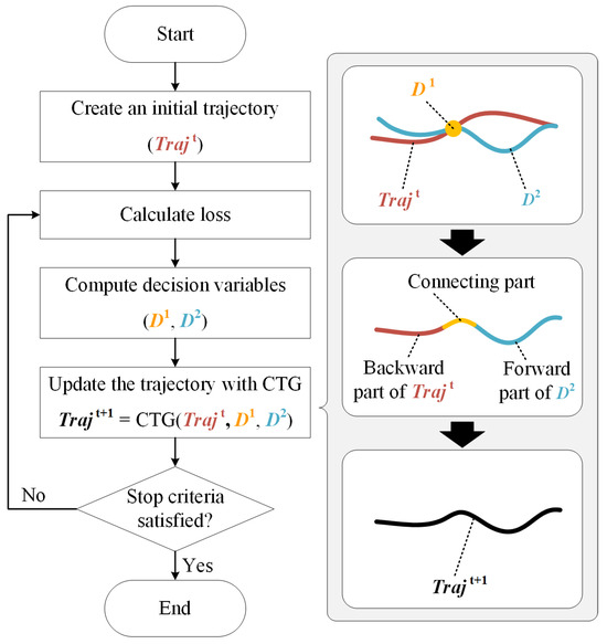
Figure 3.
Connection-based trajectory generation (CTG) in an optimization loop. and are two decision variables that describe the switch point and the alternative trajectory for the original trajectory, respectively. The CTG takes , , and the original trajectory as inputs and outputs a modified trajectory to update the optimization result.
3. Majorization–Minimization-Based Adversarial Training
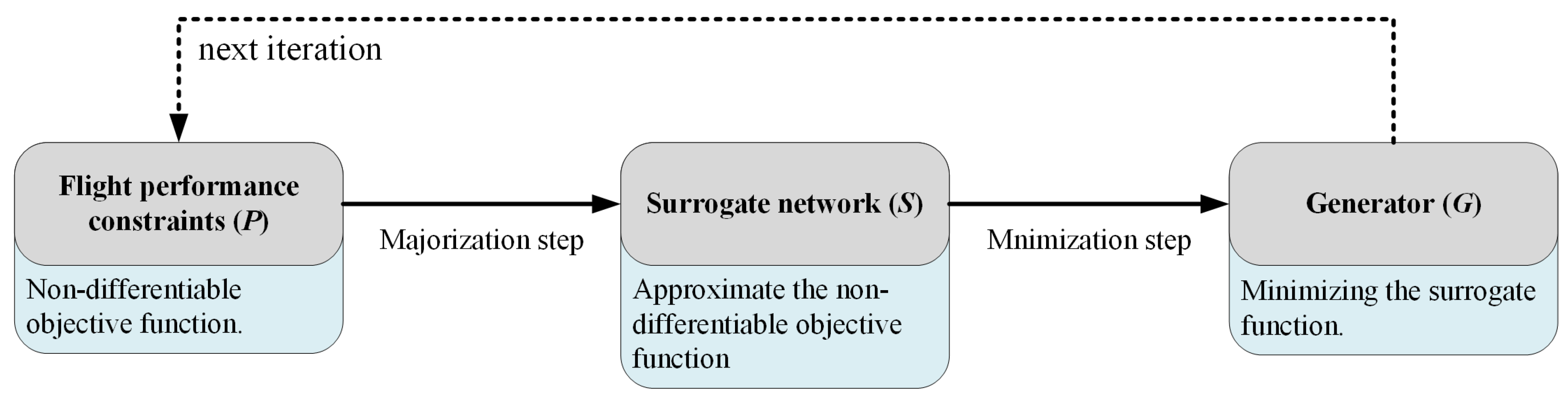
Developing a trajectory generation model that creates synthetic trajectories that meet flight performance constraints is not trivial work. Conventional neural networks should be trained with differentiable loss functions, which allows the use of gradient-based optimization methods, e.g., SGD. However, the flight performance constraints in actual operation are always non-differentiable and cannot be added to the loss functions of the neural networks. As a result, many previous data-driven trajectory generation models cannot consider flight performance constraints in the training process. To tackle this challenge, this paper exploits the MM algorithm [50] to approximate non-differentiable flight performance constraints with a differentiable neural network.
As shown in Figure 4, the proposed MMAT includes two steps. In the majorization step, the MMAT works by finding a surrogate network that could approximate the non-differentiable objective function (flight performance constraints). Then, in the minimization step, the MMAT works by finding a generator that could minimize the surrogate network. MMAT can indirectly train the generator with the non-differentiable flight performance constraints by iteratively performing the majorization and minimization steps.
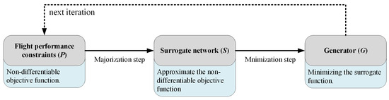
Figure 4.
Schematic diagram of majorization–minimization-based adversarial training. In the majorization step, a surrogate network is trained to approximate the flight performance constraints; in the minimization step, a generator is trained to minimize the output of the surrogate to consider the flight performance constraints.
The convergence proof of the MMAT is presented in Appendix B. According to Appendix B, a Negative Experience Replay (NER) technique is required to ensure the convergence of the generator. Specifically, the NER technique argues that all the mistakes (connecting parts that cannot meet the flight performance constraints) made by the generator should be collected and reused while training the surrogate network. In other words, NER ensures that the generator will not make the same mistakes again.
In this paper, the surrogate network and generator are trainable neural networks, denoted as and , respectively. The subscripts and represent the surrogate network’s and generator’s trainable parameters, respectively. Section 3.1 introduces the majorization step and the loss function of the neural network . Section 3.2 introduces the minimization step and the loss function of the neural network . Section 3.3 presents the pseudo-code for iteratively training and .
3.1. Majorization Step
This paper trained a neural network as a surrogate network to approximate the non-differentiable constraints. A schematic diagram of the majorization step is shown in Figure 5. The parameters of the surrogate network are trainable, and the parameters of the generator are frozen.
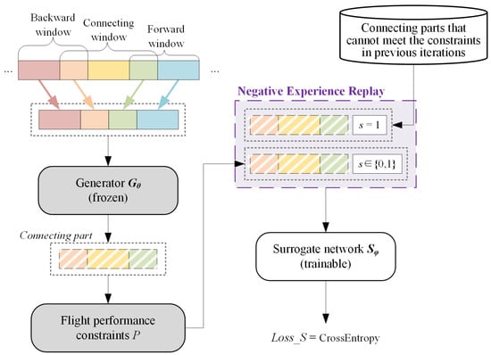
Figure 5.
Schematic diagram of the majorization step. The connecting parts generated by the generator are labeled according to the flight performance constraints and then added to the training dataset together with connecting parts that cannot meet the constraints in previous iterations. The labeled training data are used to train the supervised learning-based surrogate network, and the loss function is cross-entropy. The red, yellow, and blue boxes refer to the part of the backward, connecting, and forward trajectories that do not overlap with others, respectively. The orange and green boxes refer to the overlapping part of two adjacent trajectories.
Firstly, a batch of forward and backward parts are input into the generator , and the output of can be regarded as the predicted connecting parts. Then, these connecting parts are labeled with 0 or 1 according to whether these connecting parts can meet the flight performance constraints. For example, if a connecting part exceeds the flight performance limits, it will be labeled with 1; otherwise, it will be labeled with 0. Thirdly, the surrogate network is trained based on previously labeled data. Specifically, according to the instruction of NER, this paper uses all the labeled connecting parts in this iteration and all the connecting parts that cannot meet the constraints in previous iterations to train the surrogate network.
As shown in Equation (1), conventional cross-entropy is used as the training loss of because the surrogate network is a binary classification model.
where B is the batch size, and and are the outputs of the flight performance constraints P and surrogate network , respectively.
3.2. Minimization Step
To generate connecting parts that meet the flight performance constraints, this paper trained a neural network as a generator to minimize the outputs of the surrogate network . A schematic diagram of the minimization step is shown in Figure 6. The parameters of the generator are trainable, and the parameters of the surrogate network are frozen.
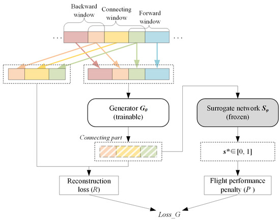
Figure 6.
A schematic diagram of the minimization step. The generator’s loss function includes reconstruction loss and a flight performance penalty. The reconstruction loss is the weighted mean square error between the real and generated connecting parts, and the flight performance penalty is the mean value of the surrogate network’s output.
Firstly, a batch of forward and backward parts are input into the generator to obtain the predicted connecting parts. According to Equation (2), the reconstruction error R can be calculated based on the predicted and real connecting parts. According to Equation (3), the approximated flight performance constraint value P can be calculated via the surrogate network . Finally, the total loss for the generator can be calculated based on Equation (4). Minimizing R encourages the predicted connecting parts to look more natural in geometry, and minimizing P encourages the predicted connecting parts to meet the flight performance constraints.
where B is the batch size, N is the length of a connecting part, is the weight of the point of the connecting part, and and are the real and predicted connecting parts, respectively. is the surrogate network whose parameters are not trainable in the minimization step, and is a non-negative coefficient.
As shown in Figure 7, the weights for both sides of a connecting part are higher than the others to ensure the connecting part can smoothly connect with the backward and forward parts.
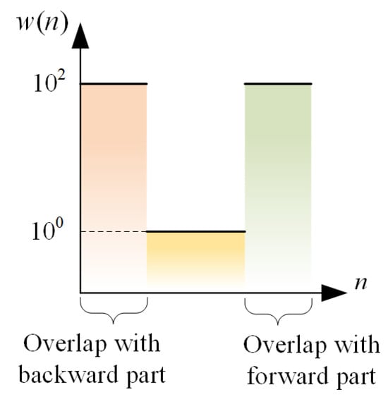
Figure 7.
Weight assignment for different trajectory points.
3.3. Implementation Details
In practice, to improve convergence, this paper separately pre-trains the generator and the surrogate network until both and are stable. Then, this paper iteratively fine-tunes and . Algorithm 1 describes the pseudo-code of the MMAT training process in more detail.
However, MMAT cannot guarantee that the generated connecting parts meet the flight performance constraints. On the one hand, the generator has no strict flight performance guarantee, but only approximately satisfies those constraints by minimizing the output of the surrogate network . On the other hand, not all the backward and forward parts can be connected properly. For example, if a backward part and a forward part are far from each other, it is impossible to combine those two to obtain a new trajectory.
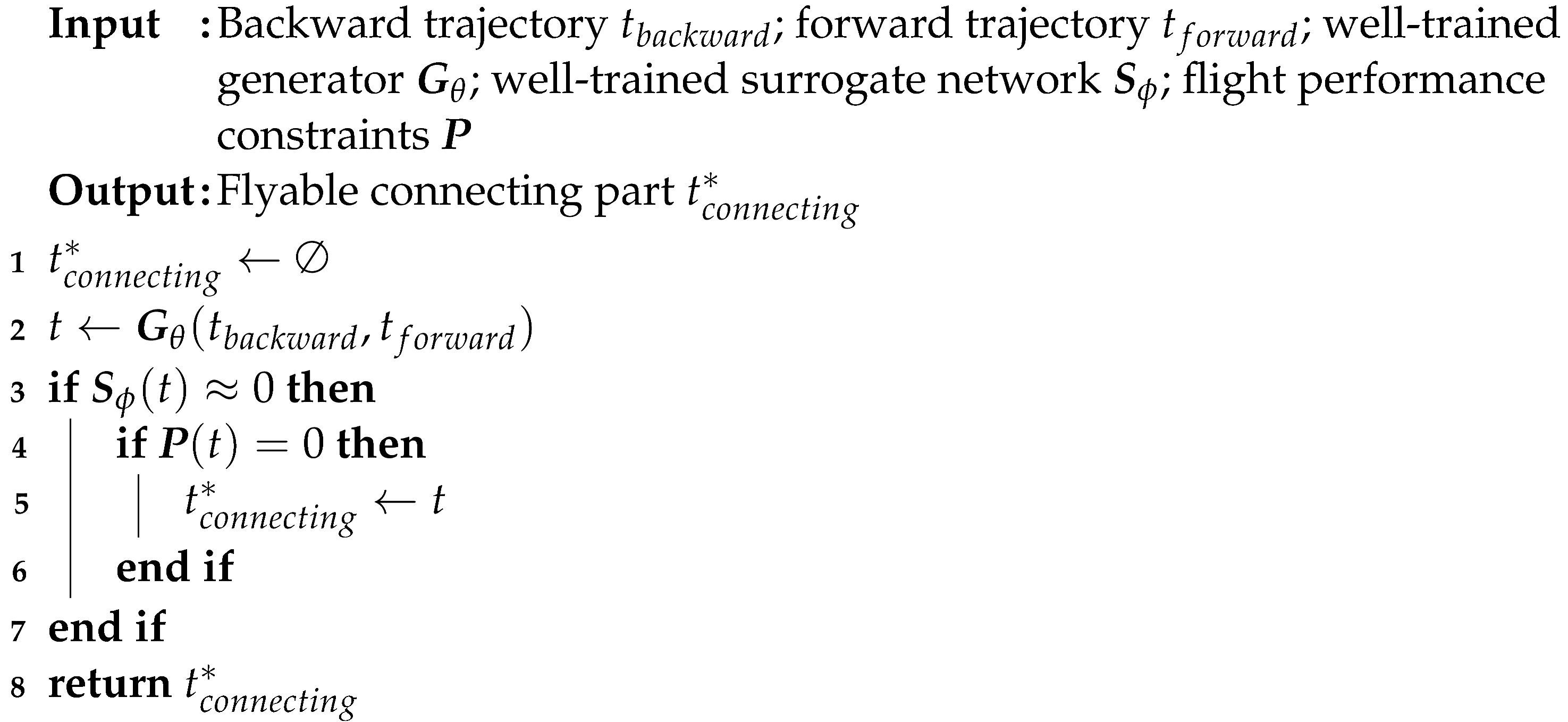
To ensure that all the generated trajectories can meet the flight performance constraints, this paper additionally introduced two-round flyable trajectory filtering to eliminate all the trajectories that cannot meet the constraints. Algorithm 2 describes the two-round flyable trajectory filtering process in more detail. Firstly, the surrogate network is exploited to quickly and roughly eliminate connecting parts that cannot be achieved. Secondly, the flight performance constraint P is used to eliminate the unflyable connecting parts.
| Algorithm 1: Pseudo-code of the training process |
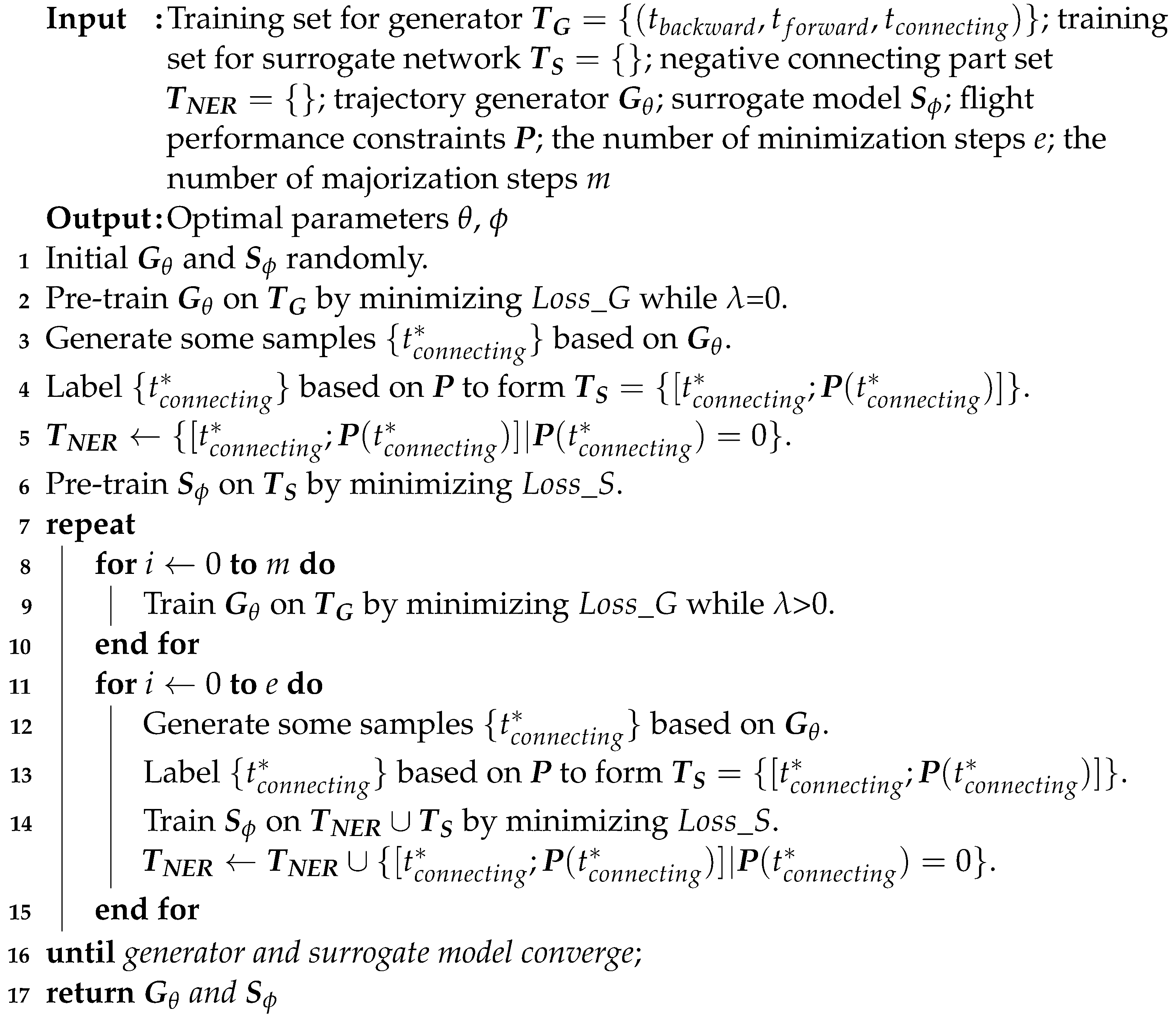 |
| Algorithm 2: Trajectory Generation Implementation |
 |
4. Experiment
4.1. Experimental Setup
Air traffic operation in the terminal area (TMA) is much more complex than in other airspaces. Arriving aircraft need to follow the instructions delivered by controllers instead of standard procedures to establish landing sequences and maintain safe separation in the TMA. As a result, arrival trajectories always have a higher diversity than departure and en-route trajectories. Thus, this paper uses the proposed CTG-MMAT to generate arrival trajectories to validate its efficiency. It is worth noting that the trajectory generation model proposed in this paper can also be used to generate departure or en-route trajectories.
In this paper, we collected trajectory data (from 1 September 2019 to 31 September 2019) from the TMA of Guangzhou Baiyun International Airport (ZGGG) to conduct our experiments. According to the statistics, there are 20,121 northbound arrival trajectories and 357 southbound arrival trajectories. As shown in Figure 8, arrival trajectories enter the TMA from six entry points: ATAGA, IGONO, P270, IDUMA, GYA, and LUPVU.
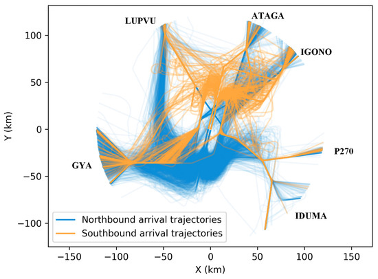
Figure 8.
Historical trajectories and six entry points.
As shown in Figure 8, arrival trajectories adopt specific maneuvers in specific areas. For example, trajectories entering from GYA prefer to take short-cut maneuvers before joining the downwind leg of the traffic pattern, and trajectories entering from ATAGA prefer to take parallel-offset maneuvers before joining the final leg of the traffic pattern. Figure 8 shows that some operation rules are contained in the collected 20,478 arrival trajectories, and CTG-MMAT should learn these rules to be considered successful. Furthermore, CTG-MMAT should also generate trajectories that meet the flight performance constraints mentioned in Section 4.2.
4.2. Flight Performance Constraints for Arriving Aircraft
In this paper, the flight performance constraints include six indicators: speed, altitude, acceleration, rate of climb, bank angle, and turning rate. Two assumptions are made when calculating these indicators:
- Due to the lack of reliable atmospheric data, this paper assumes that the wind speed is zero. According to such an assumption, the value of ground speed equals the value of true airspeed.
- To simplify computing, this paper assumes that the magnetic deviation is zero. Therefore, the value of the aircraft’s true heading is equal to the value of the aircraft’s magnetic heading.
The details of six related indicators are summarized as follows:
- Speed refers to the aircraft’s ground speed. Acceleration refers to the difference in the aircraft’s ground speed over time.
- Altitude refers to the aircraft’s pressure altitude. The rate of climb refers to the difference in the aircraft’s pressure altitude with time.
- The bank angle refers to the amount the aircraft rolls. The turning rate refers to the difference in the aircraft’s true heading with time.
- The dependencies between indicators are considered in this paper. As shown in Figure 9, speed and altitude are coupled, and the bank angle and the turning rate are also coupled.
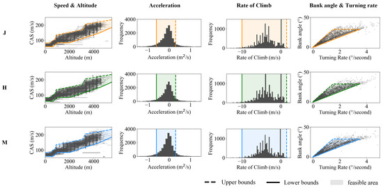 Figure 9. Flight performance of different aircraft categories. Each row in the figure represents a wake turbulence category, while each column in the figure represents one or two flight performance indicators. A trajectory meets the flight performance constraints if all its points lie in the feasible area.
If a generated connecting part is always within the feasible area, the generated trajectory’s flight performance penalty is 0. Otherwise, the generated trajectory’s flight performance penalty is 1.
According to [51,52], aircraft can be divided into four weight turbulence categories: L, M, H, and J. As shown in Figure 9, an aircraft’s flight performance depends on its weight turbulence category. Due to the lack of trajectories belonging to the L-category in the collected data, only the other three categories of aircraft (M, H, and J) are considered in Figure 9.
Although trajectories of different aircraft categories have various flight performances, as shown in Figure 9, the feasible area for various aircraft categories is the same. This phenomenon is probably because, in most cases, the standard procedures and controllers’ instructions should be suitable for any aircraft and not vary from aircraft to aircraft to reduce the associated workload. According to this finding, this paper does not specify the aircraft categories used to train the model in the following experiment.
4.3. Settings of Parameters
The computer used in this experiment was an HP desktop with an Intel Core i7-7700 at a CPU frequency of 3.60 GHz. All the code was implemented in Python 3.7.
Firstly, this paper initialized the generator by pre-training the model for 600,000 epochs by minimizing the while using an Adam [53] optimizer with a batch size of 200,000, and a learning rate of . The adapted architecture of the generator is shown in Table 1.

Table 1.
Adapted architecture of generator.
Secondly, this paper initialized the surrogate network by pre-training the model for 1,000,000 epochs by minimizing the using an Adam optimizer with a batch size of 100,000 and a learning rate of . The adapted architecture of the discriminator is shown in Table 2.
Table 2.
Adapted architecture of discriminator.
Thirdly, this paper trained the generator and surrogate network for 300,000 epochs while . Specifically, the generator was trained using an Adam optimizer with a batch size of 200,000 and a learning rate of , and the surrogate network was trained using an Adam optimizer with a batch size of 100,000 and a learning rate of .
4.4. Benchmark Model
To further demonstrate that the trajectories generated via CTG-MMAT are more likely to stay flyable, this paper compared CTG-MMAT with the state-of-the-art trajectory generation model VampPrior TCVAE proposed by [39]. VampPrior TCVAE was chosen for two reasons. First, it outperforms other models, such as the Gaussian mixture model presented in [41]; second, it is good at generating arrival trajectories.
As shown in Figure 10, VampPrior TCVAE can be regarded as a VAE architecture embedded with some improvements. Firstly, a temporal convolutional network was used to extract spatial–temporal features from trajectories; secondly, a variational mixture of posteriors was used to replace the simplistic prior (standard Gaussian).
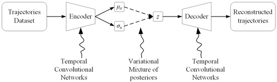
Figure 10.
The improvement made by VampPrior TCVAE. The commonly used fully connected layers in the encoder and decoder are replaced with temporal convolutional networks to better extract the spatial–temporal features from the trajectories, and the widely used standard Gaussian is replaced with the variational mixture of posteriors.
5. Results and Discussion
This section evaluates the proposed trajectory generation method to demonstrate that CTG-MMAT can be embedded with more domain knowledge. First, this paper evaluated whether the proposed MMAT technique could train the trajectory generator with non-differentiable flight performance constraints; second, this paper evaluated whether the proposed CTG framework could generate trajectories with higher diversity and fidelity by incorporating more operation experience and maneuvering rules.
5.1. Generating Trajectories with Flight Performance Constraints
To ensure flyability, the generated trajectories should meet the flight performance constraints. Therefore, this paper proposed an MMAT technique to train a generator with non-differentiable flight performance constraints.
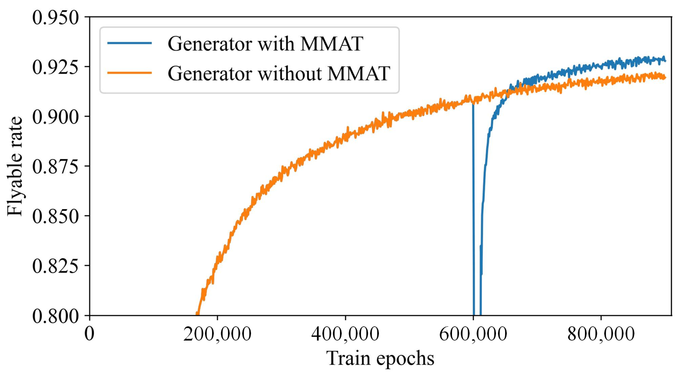
A controlled experiment is presented in this sub-section to explore whether the proposed MMAT technique enables the generator to learn more about flight performance constraints. The experiment group is the generator trained with the MMAT technique, and the control group is the generator trained without the MMAT technique. Firstly, this paper pre-trained the experiment and control groups for 600,000 epochs without the MMAT technique. Then, this paper trained the experiment group for 300,000 epochs with the MMAT technique and the control group for 300,000 epochs without the MMAT technique. The generated trajectories’ flyability changes throughout the training epochs are shown in Figure 11.
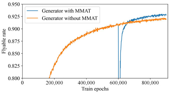
Figure 11.
Flyability changes throughout the training epochs. The MMAT technique is introduced to the experiment group after 600,000 epochs, and the flyable rate of the experiment group first sharply declines and then rapidly rebounds, and finally exceeds the control group.
Figure 11 shows that after introducing the MMAT technique, the flyable rate of the experimental group first sharply declines and then rapidly rebounds, and finally exceeds the control group. The decrease in the flyable rate is because the surrogate network was trained with biased data at the beginning of the introduction of MMAT. Fortunately, by iteratively training the generator and surrogate network, the bias of the surrogate network continues to decrease, and the MMAT technique finally shows its positive effects. The flyability changes in Figure 11 strongly suggest that the MMAT technique plays a key role in requiring the generator to consider flight performance constraints.
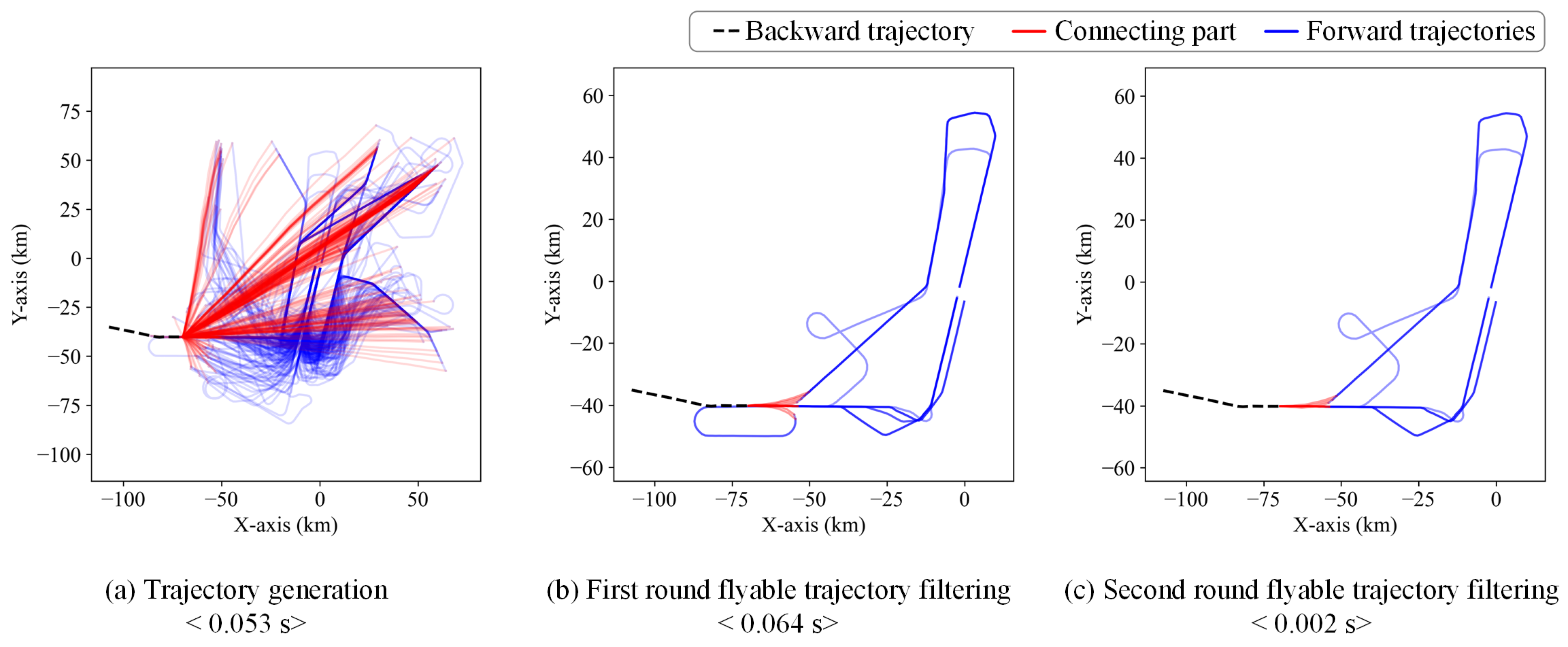
Once a well-trained generator and surrogate network are obtained, the feasible trajectories can be generated in three steps. For the first step, as shown in Figure 12a, a large number of synthetic trajectories are generated by combining the backward trajectory with randomly selected forward trajectories via the CTG framework. For the second step, as shown in Figure 12b, the well-trained surrogate network is used to conduct the first-round flyable trajectory filtering to quickly and roughly eliminate connecting parts that cannot be achieved. For the third step, as shown in Figure 12c, the flight performance constraints are used to conduct the second-round flyable trajectory filtering to precisely eliminate unflyable connecting parts. Furthermore, due to the fact that CTG-MMAT is trained offline and used online, as shown in Figure 12, generating candidate trajectories for a given backward trajectory takes about 0.053 + 0.064 + 0.002 = 0.119 s.
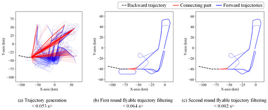
Figure 12.
Trajectory generation with the well-trained generator. (a) We randomly select some forward trajectories and connect them with the backward trajectory with connecting parts. (b) We roughly eliminate unflyable trajectories with the surrogate network. (c) We precisely eliminate unflyable trajectories according to the flight performance constraints.
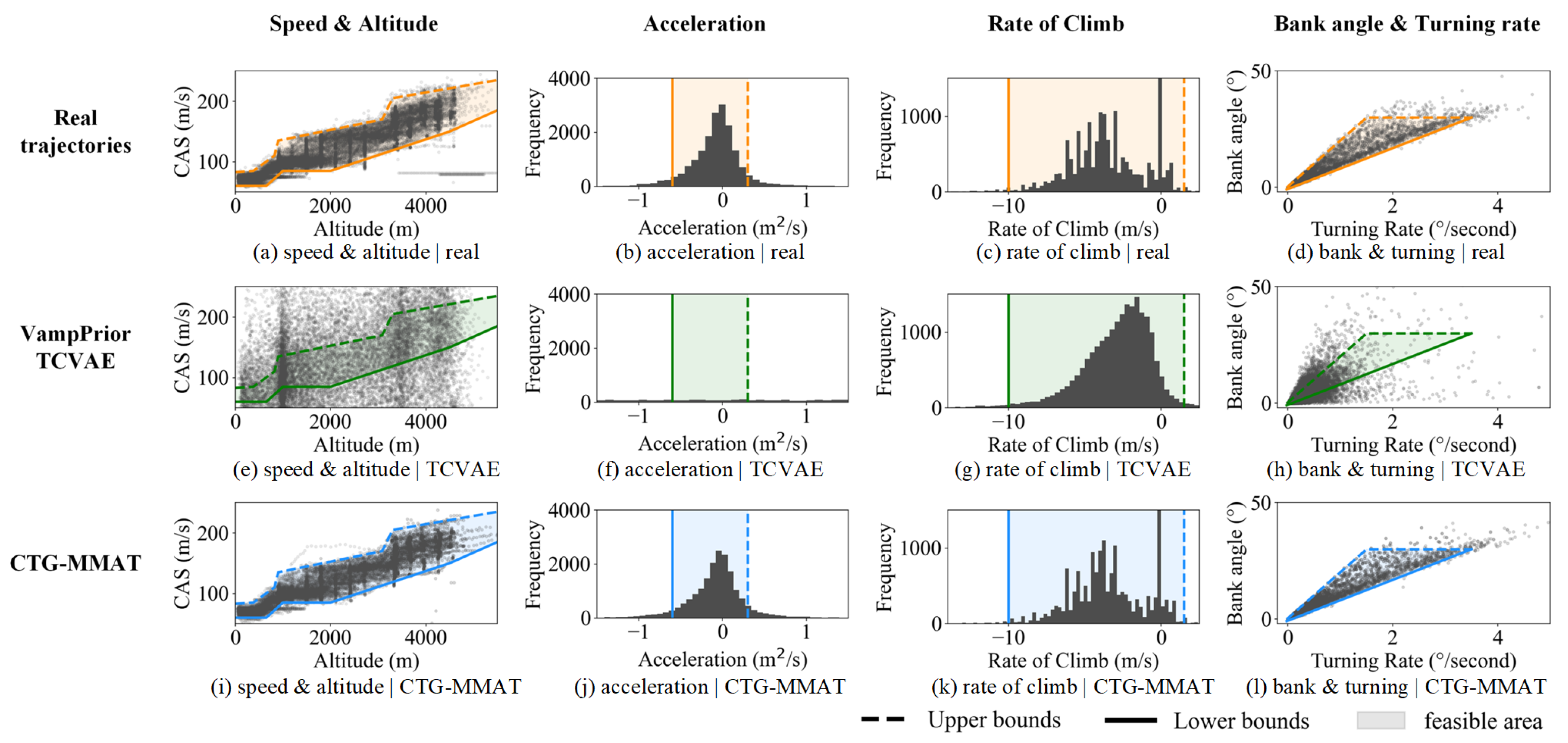
In this paper, we let CTG-MMAT and VampPrior TCVAE generate 20,000 trajectories each and calculated the flight performance parameters of those generated trajectories. It is worth noting that, according to the findings mentioned in Section 4.2, the differences in aircraft categories are ignored in this experiment. The distribution of flight performance parameters is shown in Figure 13.
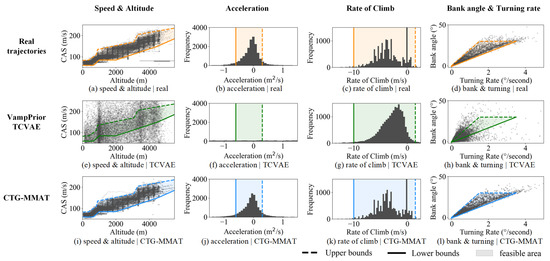
Figure 13.
Flight performance of trajectories generated by different models. Each row in the figure represents a trajectory generation model, while each column in the figure represents one or two flight performance indicators. A trajectory meets the flight performance constraints if all its points lie in the feasible area.
Figure 13e,f shows that although VampPrior TCVAE can generate high-fidelity and -diversity trajectories, the generated trajectories are often out of the feasible area. In other words, VampPrior TCVAE cannot consider flight performance constraints while generating trajectories. For example, as shown in Figure 13e, a large portion of the generated trajectories would fly at an abnormally low speed at a high altitude or at high speed at a low altitude. Compared with real trajectories’ flight performance distribution in Figure 13a–d, the distribution of trajectories generated via VampPrior TCVAE in Figure 13e,f is almost not feasible.
Figure 13e,f shows that CTG-MMAT can consider flight performance constraints since the generated trajectories are always within the feasible area. Only a few trajectory points are out of the feasible area. There are two reasons for those outliers that are out of the feasible area. First, considering that the new trajectories are generated by connecting different trajectories, those trajectory points out of the feasible area may come from the historical trajectories instead of the connecting part generated via CTG-MMAT. Second, trajectory points out of the feasible area may happen at the joint part because of an unsmooth connection. Despite these exceptions, CTG-MMAT outperforms the state-of-the-art trajectory generation model.
To summarize, with the help of the proposed MMAT technique, the proposed trajectory generation model successfully learns non-differentiable flight performance constraints and can generate trajectories that are more likely to stay flyable.
5.2. Generating Trajectories with Operation Rules
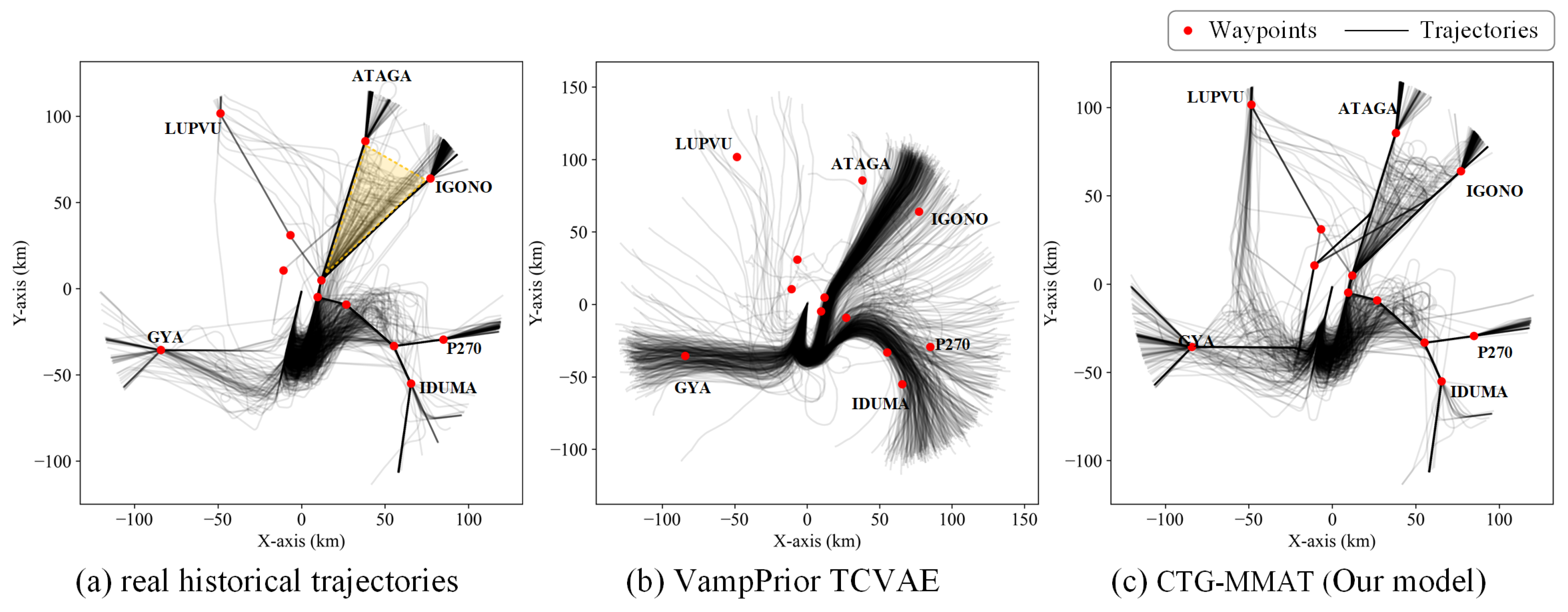
To demonstrate that CTG-MMAT can learn more operation experience, this paper compares CTG-MMAT with a state-of-the-art trajectory generation model, VampPrior TCVAE. Figure 14 shows the real historical trajectories, those generated via VampPrior TCVAE, and those generated via CTG-MMAT.
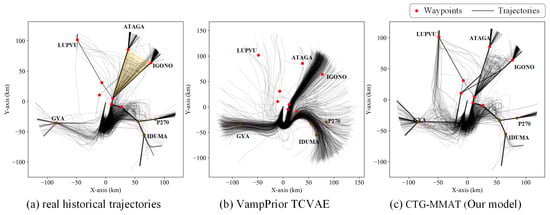
Figure 14.
Comparison with other trajectories. (a) Real northbound trajectories often pass through the published waypoints and only deviate from the published routes in specific regions. For example, an aircraft entering the TMA from ATAGA or IGONO tends to make a dog-leg in the yellow area. (b) Trajectories generated by VamPrior TCVAE ignore the published waypoints and could deviate from the published routes in any region. (c) Trajectories generated by CTG-MMAT can pass through the published waypoints and deviate at proper regions just like the real trajectories.
The real historical trajectories are shown in Figure 14a. It is easy to observe that most arriving aircraft flew over the published waypoints, denoted as red points in Figure 14, and only took necessary maneuvers in some regions. For example, arriving aircraft entered the TMA from only a few entry points rather than from any point to maintain safe separation from departure aircraft. As another example, an aircraft entering the TMA from ATAGA or IGONO tends to make a dog-leg maneuver in the yellow area in Figure 14a to postpone its landing time to establish landing sequences and maintain safe separation.
The trajectories generated via VampPrior TCVAE are shown in Figure 14b. It seems that those generated trajectories that have a similar distribution to the real ones fail to utilize operation rules even though the fidelity and diversity of these trajectories are high. For example, compared with the trajectories in Figure 14a, the generated trajectories in Figure 14b deviate from the published waypoints and occupy almost all the area of the TMA, which is strictly forbidden in the conditions of arrival and departure separation. Moreover, compared with the classic flight intentions, such as short-cut, dog-leg, hold-on, etc., the flight intentions in Figure 14b are hard to implement because the heading of these trajectories changes continuously rather than changing in steps. As a result, a pilot must constantly adjust the aircraft’s attitude to fly along such a trajectory.
In contrast, CTG-MMAT can capture operation rules quite well. Figure 14c shows trajectories generated via CTG-MMAT across the published waypoints and that have classic and easy-to-implement flight intentions, such as short-cut, dog-leg, hold-on, etc. As a result, the diversity and fidelity of trajectories generated via CTG-MMAT are high enough to be mistaken for real historical trajectories.
To summarize, the proposed CTG framework helps the trajectory generation model successfully gain more operation experience.
5.3. Generating Trajectories with Controllers’ Experience
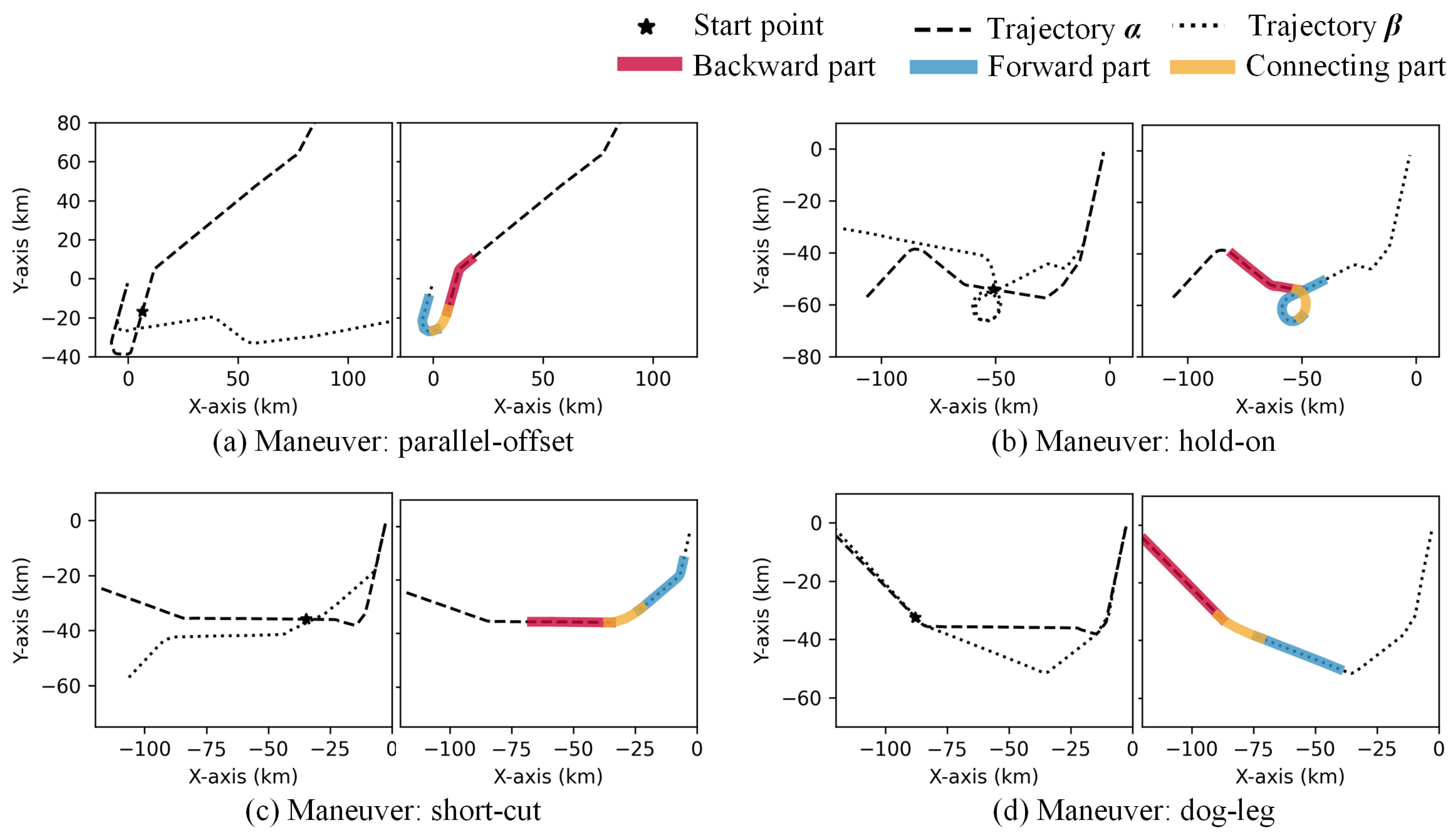
Instead of mimicking the distribution of actual trajectories, CTG generates trajectories by connecting different trajectories. As shown in Figure 15, by connecting trajectory and trajectory , the CTG framework can create trajectories with common flight intentions such as parallel-offset, hold-on, short-cut, and dog-leg.
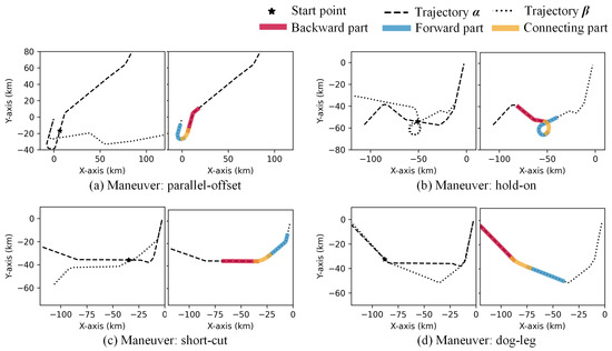
Figure 15.
Generating trajectories with different maneuvers. (a) Connecting to trajectory , which joins the base leg earlier than trajectory , to form a parallel-offset maneuver. (b) Connecting to trajectory , which has hold-on patterns, to form a hold-on maneuver. (c) Connecting to trajectory , which joins the final leg earlier than trajectory , to form a short-cut maneuver. (d) Connecting to trajectory , which has a dog-leg pattern, to form a dog-leg maneuver.
In addition, Figure 15 shows that the connecting parts partially overlap with the backward and forward parts. These overlaps are intentionally designed, as mentioned in Section 2. They can introduce data leakage while training the generator to ensure that both ends of a connecting part can seamlessly connect with the backward and forward parts. When combining these three parts to obtain a new trajectory, the overlaps should be eliminated from the connecting part.
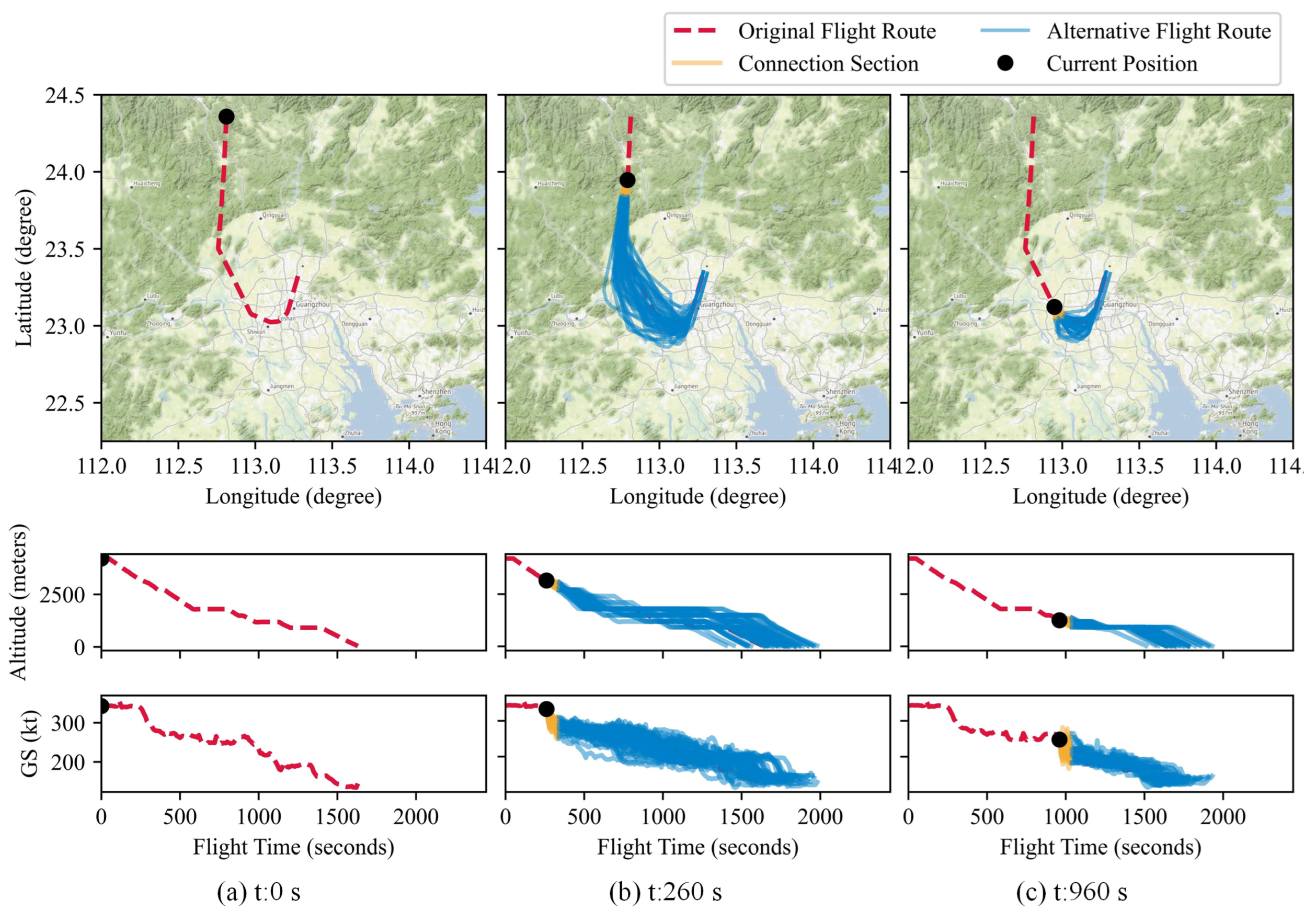
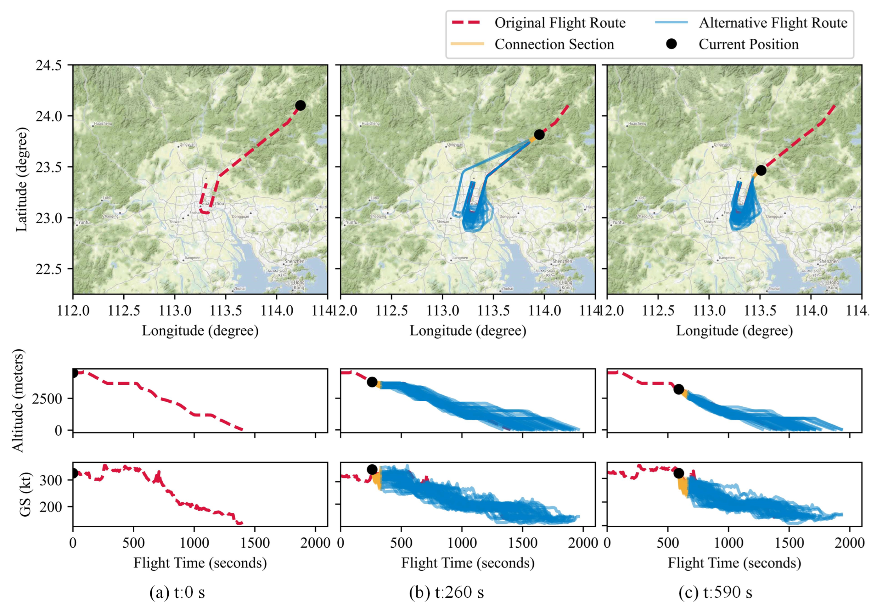
Figure 16 dynamically demonstrates the flight intention-based trajectory generation process from the perspective of pilots and controllers.
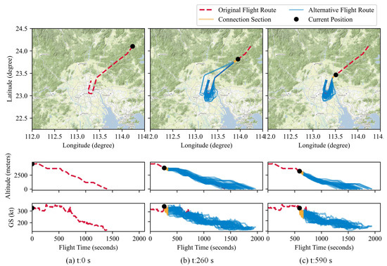
Figure 16.
Rerouting path planning for an aircraft entering from IGONO. At different positions, the ownship can switch to different historical trajectories.
As shown in Figure 16, the CTG can provide alternative arrival routes for an arriving aircraft by connecting the aircraft’s already flown trajectory with candidate historical trajectories. This connection is achieved through flight intentions such as dog-leg and short-cut. This process is close to the actual operation where a controller plans a rerouting path for an aircraft. In such cases, the CTG framework maximizes the actual operation experience while generating trajectories, since most of the content comes from historical data. Please refer to Appendix C for more examples similar to Figure 16 to show how the CTG framework recommends alternative trajectories for aircraft from different entry points.
To summarize, with the help of the proposed CTG framework, the proposed trajectory generation model can generate trajectories similar to the ones used in operations.
5.4. Lower Training Costs and Better Outcomes
The adapted architecture of the proposed generator—including only three dense layers—is quite simple and may raise concerns about their capability. Hence, more complicated architectures are considered in this subsection to analyze the effects of different architectures.
Recurrent neural networks, such as LSTM, Gated Recurrent Unit (GRU), and Bi-directional LSTM (BiLSTM), were developed to replace dense layers because these layers can effectively leverage the temporal relation information in the trajectory. In addition, the temporal convolutional network (TCN) used in [39] was also considered since it exhibits longer memory than recurrent architectures.
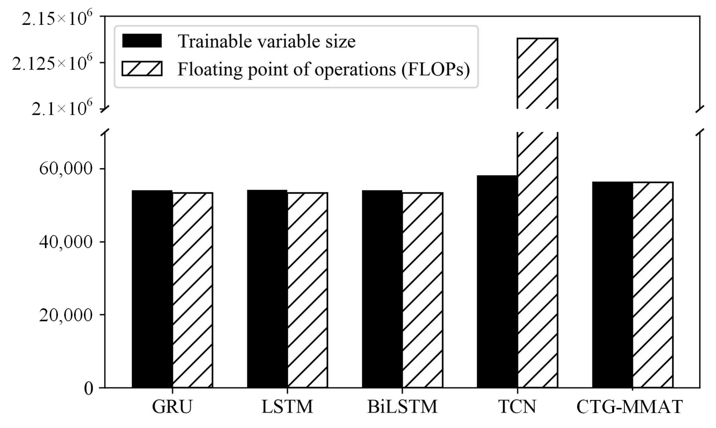
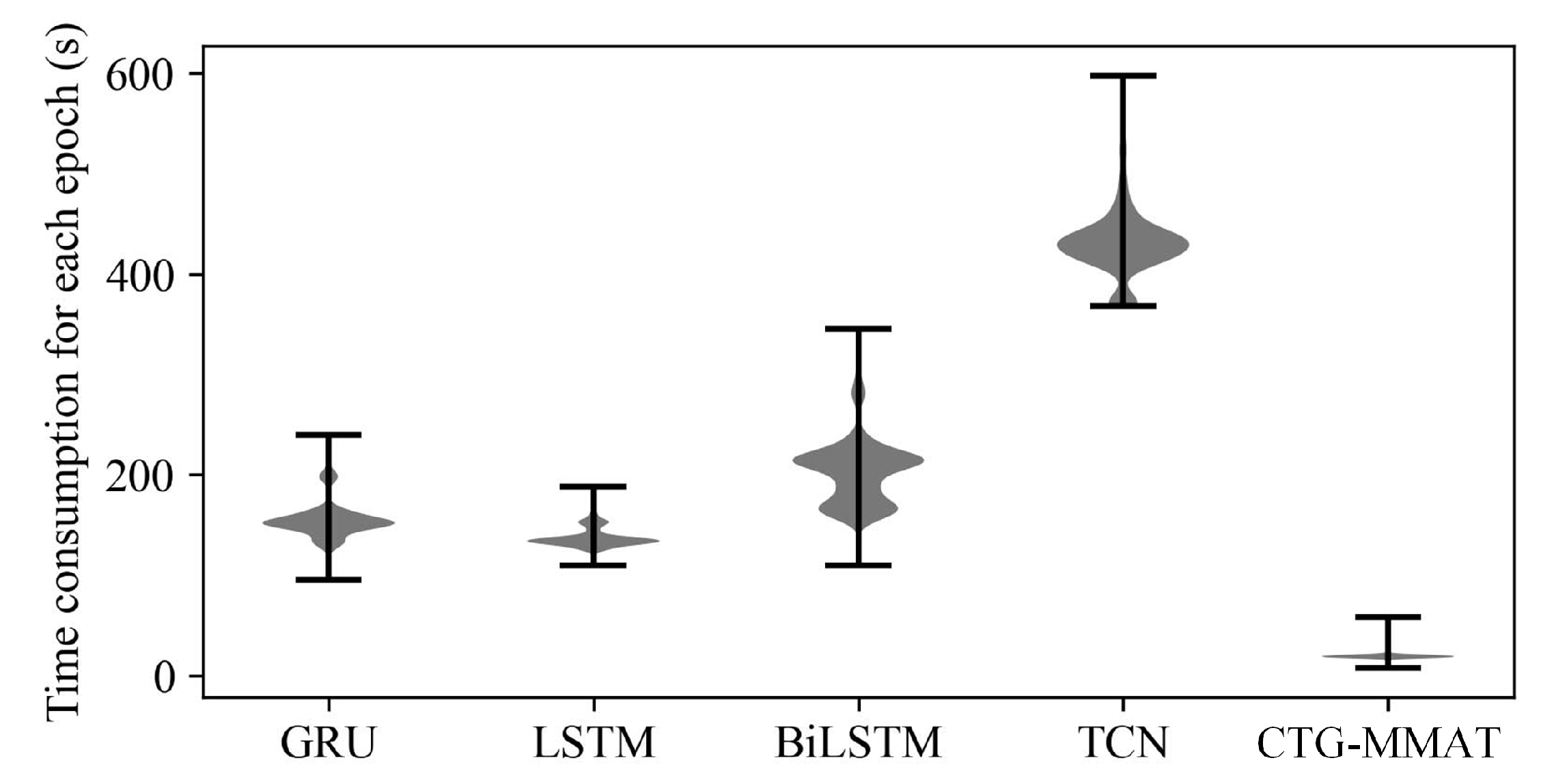
For a fair comparison, as shown in Figure 17, these models have a close number of trainable variables. However, their floating-point operations (FLOPs) differ. Specifically, the TCN’s FLOPs are about 38 times those of the other models. The higher the FLOPs, the more complex the model. In addition, as shown in Figure 18, the training time of CTG-MMAT is significantly lower than that of the other models. This is because the computations in dense layers can happen in parallel, while in the other models, they need to be processed sequentially. The simplicity of the generator matters. This explains why CTG-MMAT can be trained nearly a million times in a short time with a regular office computer. This simple neural network structure avoids dependency on high-performance deep learning workstations during the training process and lowers the bar when applying a trajectory generation model.
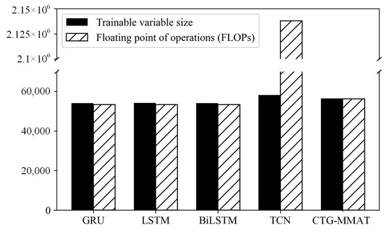
Figure 17.
Information of the models. Although the models for comparison have close trainable variable sizes, they have different FLOPs. The higher the FLOPs, the more complex the model.
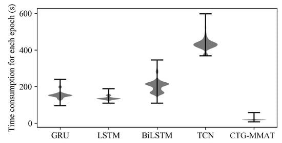
Figure 18.
Time consumption for each epoch.
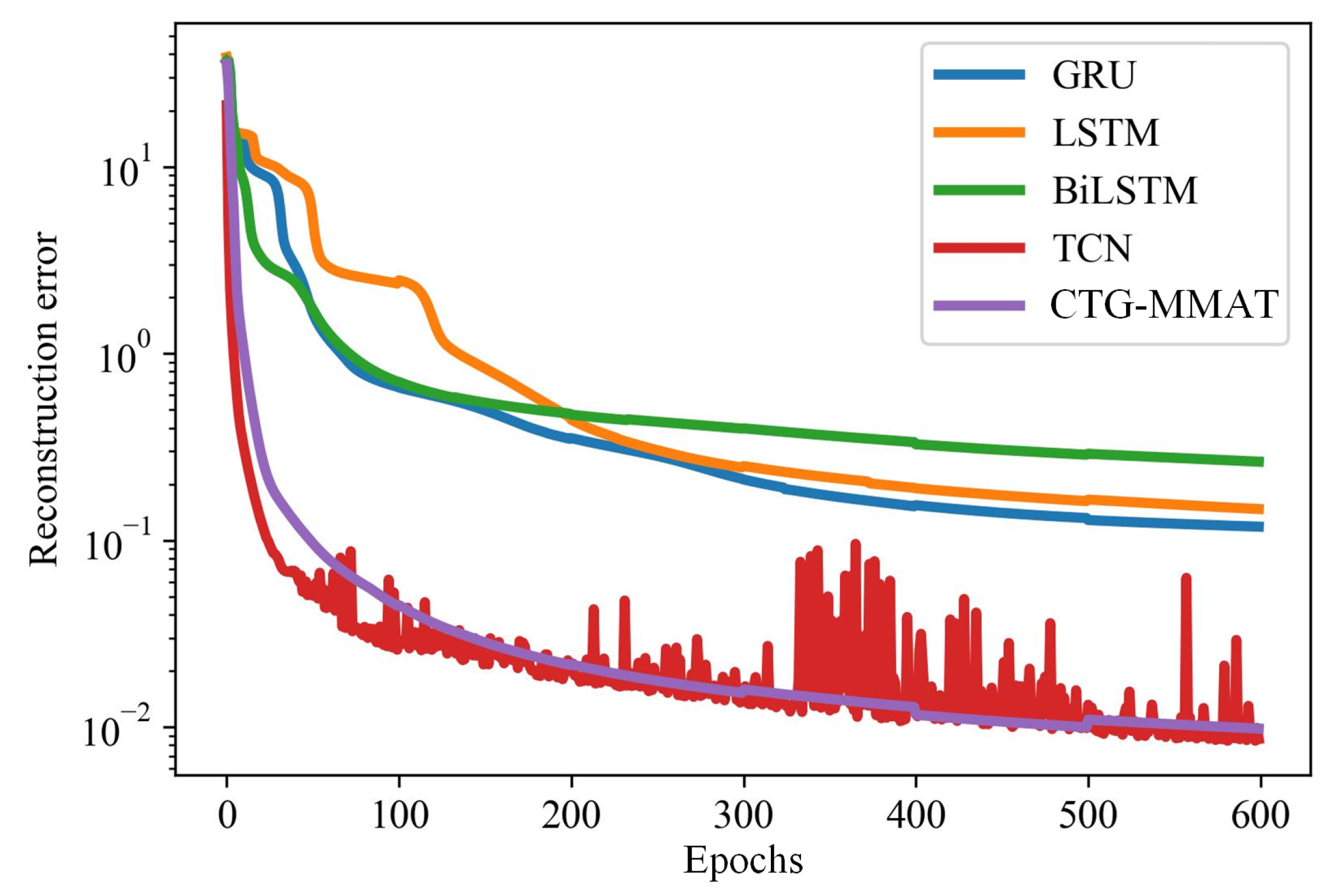
Simplifying the generator’s architecture does not always degrade its generation performance. As shown in Figure 19, the reconstruction error of CTG-MMAT is close to the best one (TCN) and outperforms the others (GRU, LSTM, BiLSTM). Although the TCN has the lowest reconstruction error, its robustness is worse than that of the other models. As shown in Figure 19, when the TCN is trained for more than 300 epochs, its reconstruction error fluctuates strongly.

Figure 19.
The variation in reconstruction error over several epochs.
Figure 20 shows the increase in the number of flyable trajectories during training. Compared with the results given in Figure 19, there is no clear relationship between the models’ reconstruction error and their ability to generate flyable trajectories: the performance of the TCN and BiLSTM differs significantly in reducing the reconstruction error, but they are similar in generating flyable trajectories. In other words, minimizing a trajectory generation model’s reconstruction error cannot guarantee that the generated trajectories are flyable, and the flight performance constraints need to be additionally considered. CTG-MMAT, which was trained to minimize both reconstruction error and flight performance penalty, is the best example. As shown in Figure 20, CTG-MMAT outperforms the other models in generating flyable trajectories.
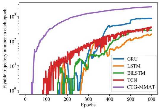
Figure 20.
The variation in flyable trajectory numbers over several epochs.
6. Conclusions
This paper proposed a novel trajectory generation method to incorporate more domain knowledge while generating trajectories, such as operation rules, controllers’ experience, and flight performance constraints. Such a generative model is of great interest in traffic-related mining and simulation since it can provide large-scale trajectory data when only a limited amount of observation is available. By incorporating the proposed CTG framework and MMAT technique, the model fulfills all expectations mentioned in the introduction:
- This paper adds non-differentiable flight performance constraints into the trajectory generation model. Considering that the non-differentiable flight performance constraints cannot be added to the trajectory model directly, the proposed model incorporates the MMAT technique to approximate non-differentiable constraints with differentiable functions to train CTG-MMAT with flight performance constraints. As a result, the trajectories generated via CTG-MMAT are more likely to be flyable than those generated using previous models.
- Unlike previous trajectory generation methods focusing on generating a whole trajectory, the proposed CTG-MMAT generates trajectories by connecting several sub-trajectories. This way, CTG-MMAT can not only fully utilize the operation rules and controllers’ experience, but can also be plugged into a combinatorial optimization algorithm to achieve trajectory optimization in the future.
- With the help of the CTG framework, the synthetic trajectory generation task becomes far easier. Accordingly, the generator composed of several dense layers is able to generate high-diversity and -fidelity trajectories. The training costs can be reduced significantly, reducing the threshold of development and application for future trajectory generation-related tasks.
Although the proposed trajectory generation method was validated by generating arrival trajectories for the ZGGG airport, it can also be directly applied to other types of trajectories. In the future, we will analyze the trajectory generation model’s robustness and integrate the proposed model into traffic-related mining and simulation tasks to improve the performance of these related algorithms.
Author Contributions
Conceptualization, X.G. and J.Z.; methodology, X.G.; software, X.G.; validation, X.G., J.B. and X.T.; formal analysis, X.T.; investigation, X.G.; resources, J.Z.; data curation, J.Z.; writing—original draft preparation, X.G.; writing—review and editing, J.Z. and D.D.; visualization, D.D.; supervision, D.D.; project administration, J.Z.; funding acquisition, J.Z. All authors have read and agreed to the published version of the manuscript.
Funding
This research was funded by the National Natural Science Foundation of China grant number 52372315, 52072174, 52002179, U1933117; and the Funds of China Scholarship Council grant number 202306830116.
Data Availability Statement
The raw data supporting the conclusions of this article will be made available by the authors on request.
Conflicts of Interest
The authors declare no conflicts of interest.
Abbreviations
The following abbreviations are used in this manuscript:
| LSTM | Long Short-Term Memory |
| VAE | Variational Auto-Encoder |
| GAN | Generative Adversarial Network |
| PCA | Principal Component Analysis |
| CTG | Connecting-based trajectory generation |
| MMAT | Majorization–minimization-based adversarial training |
| MM | Majorization–minimization |
| NER | Negative Experience Replay |
| TMA | Terminal area |
| FLOPs | Floating-point operations |
| TCN | Temporal convolutional network |
| GRU | Gated Recurrent Unit |
| BiLSTM | Bi-directional Long Short-Term Memory |
Appendix A. Sensitivity Analysis
A sensitivity analysis was conducted to determine how the model structure affects the performance of the trajectory generation model. Specifically, we synchronously changed the model’s structure and the sliding window’s size and validated the performance differences of the generator in two cases.
The first case is the training or testing case. As shown in Figure A1a, the backward and forward parts were obtained from the same trajectory through a sliding window. The second case is the application case. As shown in Figure A1b, the backward and forward parts were obtained randomly from different trajectories, not the same ones. Considering that the randomly sampled backward and forward parts in the second case may be too far apart to find a proper connecting part to combine the backward and forward trajectories, the generator’s performance in the second case will not be as good as in the first case.

Figure A1.
Input data in different cases. (a) We collect backward and forward parts from the same trajectory through a sliding window. (b) We randomly collect backward and forward parts from different trajectories.
Figure A1.
Input data in different cases. (a) We collect backward and forward parts from the same trajectory through a sliding window. (b) We randomly collect backward and forward parts from different trajectories.
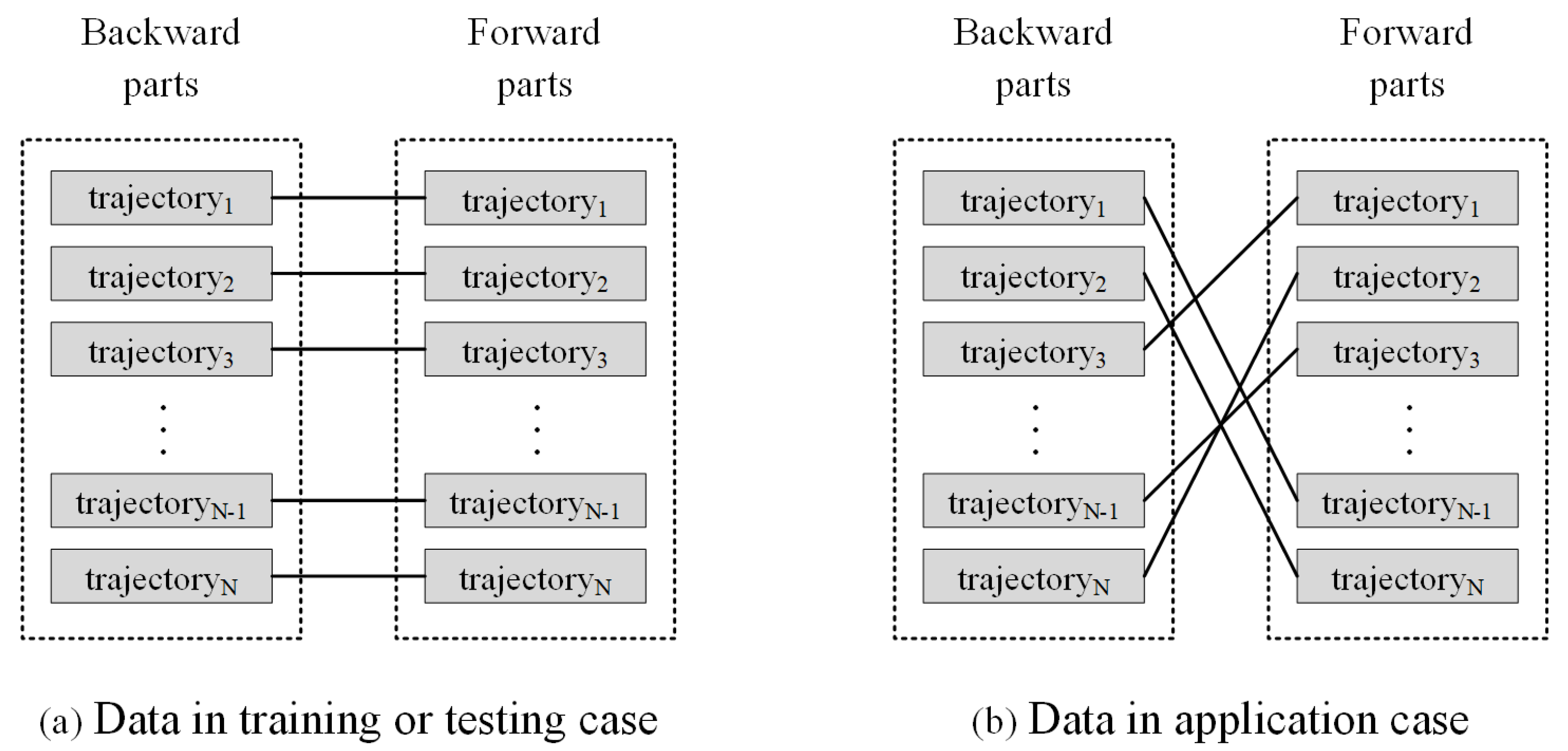
Table A1 summarizes the performance of the generator in the training and testing cases. When we changed the size of the sliding window, we obtained intuitive experimental results. On the one hand, the shorter the connecting parts, the more likely it is that the generated trajectories are feasible. One possible reason is that reducing the size of the connecting window makes the generation task easier. On the other hand, the longer the backward/forward window, the more likely it is that the generated trajectories are feasible. One possible reason is that increasing the size of the backward/forward parts brings more information for the generation step.
Table A1.
Flight performance compliance rate of generated trajectories in training and testing cases.
Table A1.
Flight performance compliance rate of generated trajectories in training and testing cases.
| Conn. | 8 | 12 | 16 | 20 | |
|---|---|---|---|---|---|
| Back./Forw. | |||||
| 4 | 94.05% | 90.96% | 90.47% | 86.43% | |
| 14 | 95.13% | 93.39% | 90.41% | 88.77% | |
| 24 | 95.41% | 93.37% | 90.67% | 88.55% | |
| 34 | 95.70% | 93.74% | 91.35% | 87.62% | |
Table A2 summarizes the performance of the generator in the application case. Due to the fact that the backward and forward parts were obtained randomly from different trajectories, the values in Table A2 are much lower than those in Table A1. Furthermore, when we changed the size of the sliding window, we obtained counterintuitive experimental results. On the one hand, the longer the connecting window, the more likely it is that the generated trajectories are feasible. One possible reason is that, in the application, the longer the connecting parts, the more forward parts can match the backward part. On the other hand, the longer the backward/forward part, the less likely it is that the generated trajectories are feasible. One possible reason is that the backward/forward parts contain distinct intentions, and increasing the length of the backward/forward parts intensifies the contradictions between the two flight intentions.
Table A1 suggests that the generation task will be more successful when decreasing the length of the connecting part and increasing the length of the backward/forward parts. Table A2 suggests that the model will be more practical when increasing the length of the connecting part and decreasing the length of the backward/forward parts. To make a trade-off between training cost and practicability, we set the length of the connecting part to 12 and the backward/forward parts to 24.
Table A2.
Flight performance compliance rate of generated trajectories in application case.
Table A2.
Flight performance compliance rate of generated trajectories in application case.
| Conn. | 8 | 12 | 16 | 20 | |
|---|---|---|---|---|---|
| Back./Forw. | |||||
| 4 | 0.70% | 1.01% | 1.68% | 2.03% | |
| 14 | 0.41% | 0.78% | 1.18% | 1.46% | |
| 24 | 0.31% | 0.49% | 0.82% | 1.27% | |
| 34 | 0.17% | 0.39% | 0.61% | 0.92% | |
Appendix B. Convergence Proof and Negative Experience Replay
To train a generator with flight performance constraints, the loss function of the generator can be written as a functional.
where is the connecting part generator, P is the flight performance constraints, B is the batch size, and and are the backward and forward parts, respectively.
According to Equation (A1), we have:
In most cases, P is complicated and non-differentiable, so P cannot be used to train the generator directly. Therefore, we transform the trajectory generation problem into a majorization–minimization problem.
Instead of operating on P, we train a surrogate network to approximate P. Noting that is a neural network, we have:
where is the modified loss functional in which P is replaced by .
According to the definition of MM, the surrogate network should meet the following two essential conditions to ensure convergence:
where and are the generator and surrogate network in iterate, respectively, and is the generator at iteration t.
The remainder of this appendix proposes a Negative Experience Replay (NER) technique to ensure that can meet the two conditions mentioned above. For the convenience of illustration, we rewrite Equations (A4) and (A5).
Firstly, Equation (A4) requires that the be consistent with P in flight performance penalty evaluation for . Hence, Equation (A4) can be rewritten as follows:
where is the set of connecting parts that can meet the flight performance constraints, and is the set of connecting parts that cannot meet the flight performance constraints. Both and are generated by .
Secondly, Equation (A5) requires that retain some memory during iteration. Specifically, should consider the unflyable connecting parts generated by – as ones that cannot meet the flight performance constraints. Therefore, Equation (A5) can be rewritten as follows:
where is the set of connecting parts that cannot meet the flight performance constraints. is generated by all previous generators –.
Based on Equation (A6)–(A8), we can summarize the NER technique: train with not only trajectories generated by , but also unflyable connecting parts generated by –. In the practice of NER, we construct the training set with all the unflyable connecting parts and the same number of flyable connecting parts.
Appendix C. Trajectory Generation for Arriving Aircraft
Five trajectory sets are given to show how CTG-MMAT recommends alternative trajectories from different entry fixes.
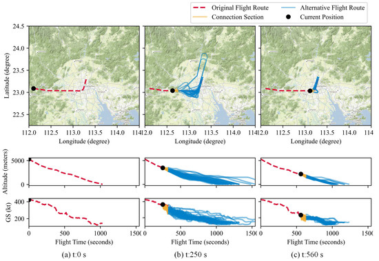
Figure A2.
Rerouting path planning for an aircraft entering from GYA. At different positions, the ownship can switch to different historical trajectories.
Figure A2.
Rerouting path planning for an aircraft entering from GYA. At different positions, the ownship can switch to different historical trajectories.
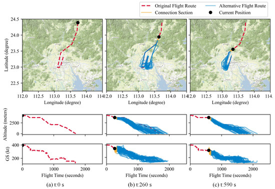
Figure A3.
Rerouting path planning for an aircraft entering from ATAGA. At different positions, the ownship can switch to different historical trajectories.
Figure A3.
Rerouting path planning for an aircraft entering from ATAGA. At different positions, the ownship can switch to different historical trajectories.

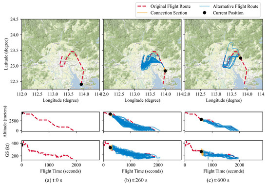
Figure A4.
Rerouting path planning for an aircraft entering from IDUMA. At different positions, the ownship can switch to different historical trajectories.
Figure A4.
Rerouting path planning for an aircraft entering from IDUMA. At different positions, the ownship can switch to different historical trajectories.

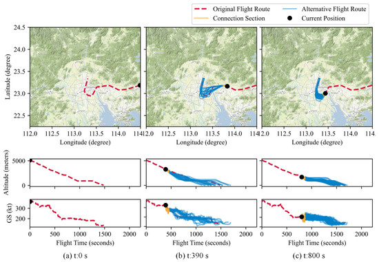
Figure A5.
Rerouting path planning for an aircraft entering from P270. At different positions, the ownship can switch to different historical trajectories.
Figure A5.
Rerouting path planning for an aircraft entering from P270. At different positions, the ownship can switch to different historical trajectories.


Figure A6.
Rerouting path planning for an aircraft entering from LUPVU. At different positions, the ownship can switch to different historical trajectories.
Figure A6.
Rerouting path planning for an aircraft entering from LUPVU. At different positions, the ownship can switch to different historical trajectories.
References
- Sun, J.; Xu, J.; Zhou, R.; Zheng, K.; Liu, C. Discovering expert drivers from trajectories. In Proceedings of the 2018 IEEE 34th International Conference on Data Engineering (ICDE), Paris, France, 16–19 April 2018. [Google Scholar]
- Zhang, P.; Zheng, J.; Lin, H.; Liu, C.; Zhao, Z.; Li, C. Vehicle Trajectory Data Mining for Artificial Intelligence and Real-Time Traffic Information Extraction. IEEE Trans. Intell. Transp. Syst. 2023, 24, 13088–13098. [Google Scholar] [CrossRef]
- Hodges, C.; An, S.; Rahmani, H.; Bennamoun, M. Deep Learning for Driverless Vehicles. In Handbook of Deep Learning Applications; Balas, V., Roy, S., Sharma, D., Samui, P., Eds.; Springer: Cham, Switzerland, 2019; pp. 83–99. [Google Scholar]
- Ding, P.; Liu, G.; Wang, Y.; Zheng, K.; Zhou, X. A-MCTS: Adaptive Monte Carlo Tree Search for Temporal Path Discovery. IEEE Trans. Knowl. Data Eng. 2023, 35, 2243–2257. [Google Scholar] [CrossRef]
- Chen, J.; Zhang, C.; Luo, J.; Xie, J.; Wan, Y. Driving Maneuvers Prediction Based Autonomous Driving Control by Deep Monte Carlo Tree Search. IEEE Trans. Intell. Veh. 2020, 69, 7146–7158. [Google Scholar] [CrossRef]
- Deng, C.; Choi, H.C.; Park, H.; Hwang, I. Trajectory pattern identification and classification for real-time air traffic applications in Area Navigation terminal airspace. Transp. Res. Part C Emerg. Technol. 2022, 142, 103765. [Google Scholar] [CrossRef]
- Andrienko, G.; Andrienko, N.; Fuchs, G.; Cordero Garcia, J.M. Clustering trajectories by relevant parts for air traffic analysis. IEEE Trans. Vis. Comput. Graph. 2018, 24, 34–44. [Google Scholar] [CrossRef] [PubMed]
- Murça, M.C.R.; Hansman, R.J.; Li, L.; Ren, P. Flight trajectory data analytics for characterization of air traffic flows: A comparative analysis of terminal area operations between New York, Hong Kong and Sao Paulo. Transp. Res. Part C Emerg. Technol. 2018, 97, 324–347. [Google Scholar] [CrossRef]
- Delahaye, D.; Puechmorel, S.; Alam, S.; Féron, E. Trajectory mathematical distance applied to airspace major flows extraction. In Proceedings of the 5th ENRI International Workshop on ATM/CNS 2017, Nakano, Japan, 14–16 November 2017. [Google Scholar]
- Jacquemart, D.; Morio, J. Adaptive interacting particle system algorithm for aircraft conflict probability estimation. Aerosp. Sci. Technol. 2016, 55, 431–438. [Google Scholar] [CrossRef]
- Gui, X.; Zhang, J.; Tang, X.; Bao, J.; Wang, B. A data-driven trajectory optimization framework for terminal maneuvering area operations. Aerosp. Sci. Technol. 2022, 131, 108010. [Google Scholar] [CrossRef]
- Ma, J.; Zhou, J.; Liang, M.; Delahae, D. Data-driven trajectory-based analysis and optimization of airport surface movement. Transp. Res. Part C Emerg. Technol. 2022, 145, 103902. [Google Scholar] [CrossRef]
- Olive, X.; Sun, J.; Murça, M.C.R.; Krauth, T. A Framework to Evaluate Aircraft Trajectory Generation Methods. In Proceedings of the Fourteenth USA/Europe Air Traffic Management Research and Development Seminar, New Orleans, LA, USA, 20–24 September 2021. [Google Scholar]
- Sun, J.; Ellerbroek, J.; Hoekstra, J.M. WRAP: An open-source kinematic aircraft performance model. Transp. Res. Part C Emerg. Technol. 2019, 98, 118–138. [Google Scholar] [CrossRef]
- Zhang, J.; Liu, J.; Hu, R.; Zhu, H. Online four dimensional trajectory prediction method based on aircraft intent updating. Aerosp. Sci. Technol. 2018, 77, 774–787. [Google Scholar] [CrossRef]
- User Manual for the Base of Aircraft Data (BADA). Available online: https://www.eurocontrol.int/publication/user-manual-base-aircraft-data-bada (accessed on 1 July 2014).
- Sun, J.; Hoekstra, J.M.; Ellerbroek, J. OpenAP: An Open-Source Aircraft Performance Model for Air Transportation Studies and Simulations. Aerospace 2020, 7, 104. [Google Scholar] [CrossRef]
- Chen, Y.; Hu, M.; Yang, L. Autonomous planning of optimal four-dimensional trajectory for real-time en-route airspace operation with solution space visualization. Transp. Res. Part C Emerg. Technol. 2022, 140, 103701. [Google Scholar] [CrossRef]
- Kasmi, H.; Laporte, S.; Mongeau, M.; Vidosavljevic, A.; Delahaye, D. Holistic Approach for Aircraft Trajectory Optimization Using Optimal Control. J. Aircr. 2023, 60, 1302–1313. [Google Scholar] [CrossRef]
- Schnitzler, B.; Drouin, A.; Moschetta, J.M.; Delahaye, D. General Extremal Field Method for Time-Optimal Trajectory Planning in Flow Fields. IEEE Control Syst. Lett. 2023, 7, 2605–2610. [Google Scholar] [CrossRef]
- Ruigrok, R.C.; Hoekstra, J.M. Human factors evaluations of free flight: Issues solved and issues remaining. Appl. Ergon. 2007, 38, 437–455. [Google Scholar] [CrossRef] [PubMed]
- Kahne, S. Research issues in the transition to free flight. Annu. Rev. Control 2000, 24, 21–29. [Google Scholar] [CrossRef]
- Liang, M.; Delahaye, D.; Marechal, P. Integrated sequencing and merging aircraft to parallel runways with automated conflict resolution and advanced avionics capabilities. Transp. Res. Part C Emerg. Technol. 2017, 82, 268–291. [Google Scholar] [CrossRef]
- Sáez, R.; Prats, X.; Polishchuk, T.; Polishchuk, V. Traffic synchronization in terminal airspace to enable continuous descent operations in trombone sequencing and merging procedures: An implementation study for Frankfurt airport. Transp. Res. Part C Emerg. Technol. 2020, 121, 102875. [Google Scholar] [CrossRef]
- Sáez, R.; Prats, X.; Polishchuk, T.; Polishchuk, V.; Schmidt, C. Automation for separation with continuous descent operations: Dynamic aircraft arrival routes. J. Air Transp. 2020, 144, 144–291. [Google Scholar] [CrossRef]
- Sáez, R.; Polishchuk, T.; Schmidt, C.; Hardell, H.; Smetanova, L.; Polishchuk, V.; Prats, X. Automated sequencing and merging with dynamic aircraft arrival routes and speed management for continuous descent operations. Transp. Res. Part C Emerg. Technol. 2021, 132, 103402. [Google Scholar] [CrossRef]
- Chen, X.; Xu, J.; Zhou, R.; Chen, W.; Fang, J.; Liu, C. TrajVAE: A variational autoencoder model for trajectory generation. Neurocomputing 2021, 428, 332–339. [Google Scholar] [CrossRef]
- Choi, S.; Kim, J.; Yeo, H. TrajGAIL: Generating urban vehicle trajectories using generative adversarial imitation learning. Transp. Res. Part C Emerg. Technol. 2021, 128, 103091. [Google Scholar] [CrossRef]
- Kim, J.W.; Jang, B. Deep learning-based privacy-preserving framework for synthetic trajectory generation. J. Netw. Comput. Appl. 2022, 206, 103459. [Google Scholar] [CrossRef]
- Rao, J.; Gao, S.; Kang, Y.; Huang, Q. LSTM-TrajGAN: A deep learning approach to trajectory privacy protection. In Proceedings of the 11th International Conference on Geographic Information Science, Poznań, Poland, 15–18 September 2020. [Google Scholar]
- Wang, X.; Liu, X.; Lu, Z.; Yang, H. Large scale GPS trajectory generation using map based on two stage GAN. J. Data Sci. 2021, 19, 126–141. [Google Scholar] [CrossRef]
- LeCun, Y.; Bengio, Y.; Hintion, G. Deep learning. Nature 2015, 521, 436–444. [Google Scholar] [CrossRef] [PubMed]
- Hochreiter, S.; Schmidhuber, J. LSTM can solve hard long time lag problems. In Proceedings of the 9th International Conference on Neural Information Processing Systems, Denver, CO, USA, 3–4 December 1996. [Google Scholar]
- LeCun, Y.; Bottou, L.; Bengio, Y.; Haffner, P. Gradient-based learning applied to document recognition. Proc. IEEE 1998, 86, 2278–2324. [Google Scholar] [CrossRef]
- Kingma, D.P.; Welling, M. Auto-Encoding Variational Bayes. In Proceedings of the International Conference on Learning Representations (ICLR) 2014, Banff, AB, Canada, 3–4 December 1996. [Google Scholar]
- Goodfellow, I.; Pouget-Abadie, J.; Mirza, M.; Xu, B.; Warde-Farley, D.; Ozair, S.; Couriville, A.; Bengio, Y. Generative adversarial nets. In Proceedings of the Advances in Neural Information Processing Systems 27, Montreal, QC, Canada, 8–13 December 2014. [Google Scholar]
- Tomczak, J.M.; Welling, M. VAE with a VampPrior. In Proceedings of the 21st International Conference on Artifi cial Intelligence and Statistics (AISTATS) 2018, Lanzarote, Spain, 9–11 April 2018. [Google Scholar]
- Gulrajani, I.; Ahmed, F.; Arjovsky, M.; Dumoulin, V.; Courville, A. Improved Training of Wasserstein GANs. In Proceedings of the the 31st International Conference on Neural Information Processing Systems, Long Beach, CA, USA, 4–9 December 2017. [Google Scholar]
- Krauth, T.; Lafage, A.; Morio, J.; Olive, X.; Waltert, M. Deep generative modelling of aircraft trajectories in terminal maneuvering areas. Mach. Learn. Appl. 2023, 11, 100446. [Google Scholar] [CrossRef]
- Wu, X.; Yang, H.; Chen, H.; Hu, Q.; Hu, H. Long-term 4D trajectory prediction using generative adversarial networks. Transp. Res. Part C Emerg. Technol. 2022, 136, 103554. [Google Scholar] [CrossRef]
- Murça, M.C.R.; de Oliveira, M.W. A Data-Driven Probabilistic Trajectory Model for Predicting and Simulating Terminal Airspace Operations. In Proceedings of the the 39th IEEE/AIAA Digital Avionics Systems Conference, San Antonio, TX, USA, 11–15 October 2020. [Google Scholar]
- Henry, M.; Schmitz, S.; Kelbaugh, K.; Revenko, N. A Monte Carlo Simulation for Evaluating Airborne Collision Risk in Intersecting Runways. In Proceedings of the AIAA Modeling and Simulation Technologies (MST) Conference 2013, Boston, MA, USA, 19–22 August 2013. [Google Scholar]
- Jarry, G.; Hassoumi, A.; Delahaye, D.; Hurter, C. Interactive trajectory modification and generation with FPCA. CEAS Aeronaut. J. 2022, 13, 371–383. [Google Scholar] [CrossRef]
- Guan, Y.; Ren, Y.; Sun, Q.; Li, S.E.; Ma, H.; Duan, J.; Dai, Y.; Cheng, B. Integrated Decision and Control: Toward Interpretable and Computationally Efficient Driving Intelligence. IEEE Trans. Cybern. 2021, 53, 859–873. [Google Scholar] [CrossRef] [PubMed]
- Ma, H.; Chen, J.; Li, S.E.; Lin, Z.; Guan, Y.; Ren, Y.; Zheng, S. Model-based constrained reinforcement learning using generalized control barrier function. In Proceedings of the IEEE/RSJ International Conference on Intelligent Robots and Systems (IROS) 2021, Prague, Czech Republic, 27 September–1 October 2021. [Google Scholar]
- Ortega, J.; Rheinboldt, W. Iterative solution of nonlinear equations in several variables. In Classics in Applied Mathematics; Brenner, S., Callaghan, P., Eds.; Society for Industrial and Applied Mathematics: Philadelphia, PA, USA, 2014. [Google Scholar]
- Peng, B.; Mu, Y.; Guan, Y.; Li, S.E.; Yin, Y.; Chen, J. Model-based actor-critic with chance constraint for stochastic system. In Proceedings of the 60th IEEE Conference on Decision and Control, Austin, TX, USA, 14–17 December 2021. [Google Scholar]
- Ren, Y.; Zhan, G.; Tang, L.; Li, S.E.; Jiang, J.; Li, K.; Duan, J. Improve generalization of driving policy at signalized intersections with adversarial learning. Transp. Res. Part C Emerg. Technol. 2023, 152, 104161. [Google Scholar] [CrossRef]
- Xiao, W.; Wang, T.H.; Hasani, R.; Chahine, M.; Amini, A.; Li, X.; Rus, D. BarrierNet: Differentiable Control Barrier Functions for Learning of Safe Robot Control. IEEE Trans. Robot. 2023, 39, 2289–2307. [Google Scholar] [CrossRef]
- Sun, Y.; Babu, P.; Palomar, D.P. Majorization-Minimization Algorithms in Signal Processing, Communications, and Machine Learning. IEEE Trans. Signal Process. 2017, 65, 794–816. [Google Scholar] [CrossRef]
- Airbus A380 Wake Vortex Guidance. Available online: https://skybrary.aero/articles/airbus-a380-wake-vortex-guidance (accessed on 25 May 2024).
- Procedures for Air Navigation Services—Air Traffic Management (PANS-ATM Doc 4444). Available online: https://www.icao.int/ESAF/Documents/meetings/2021/AFI%20ATM%20Coordination%20Meeting%202021/Presentations/4444_16ed_amend_10_highlighted.pdf (accessed on 25 May 2024).
- Kingma, D.P.; Ba, J.L. Adam: A method for stochastic optimization. In Proceedings of the 3rd International Conference on Learning Representations, San Diego, CA, USA, 7–9 May 2015. [Google Scholar]


Disclaimer/Publisher’s Note: The statements, opinions and data contained in all publications are solely those of the individual author(s) and contributor(s) and not of MDPI and/or the editor(s). MDPI and/or the editor(s) disclaim responsibility for any injury to people or property resulting from any ideas, methods, instructions or products referred to in the content. |
© 2024 by the authors. Licensee MDPI, Basel, Switzerland. This article is an open access article distributed under the terms and conditions of the Creative Commons Attribution (CC BY) license (https://creativecommons.org/licenses/by/4.0/).