Framework for Numerical 6DOF Simulation with Focus on a Wing Deforming UAV in Perch Landing ^†

Abstract

The perch landing maneuver of a wing-deforming unmanned aerial vehicle (UAV) was investigated through a framework that uses the free, open-source OpenFOAM with 6 degrees of freedom (6DOF) simulations. The framework uses a moving grid to follow the trajectory of the UAV, reducing computational resources. Together with the ability to allow internal grid deformation, sliding mesh, and algorithm addition, it can accurately mimic the entire landing process. Different wing deformation speeds, additional elevator rotation and emulated propeller lift were added to the 6DOF simulations to investigate their effects on the landing maneuver. The results showed that the wing deformation retraction speed has a considerable effect on the trajectory and velocity of the UAV. The wing deformation reduced the forward velocity of the UAV by 32%, from 13.89 to 9 m/s. With the elevator control, the velocity was reduced to 5 m/s. Lastly, and an activation time of 1 s for the emulated propeller lift can further decrease the velocity to around 4.2 m/s. A better algorithm for the emulated propeller lift may be able to give a superior performance. This framework allows us to understand the underlying perch landing maneuver aerodynamics. It can also be used on problems like fast-turning agile and flapping wing flight.

1. Introduction

Perch landing in birds is considered an important but difficult maneuver. It uses a high angle of attack (AoA) to create a high drag force to achieve a short and controlled landing. This feature makes perching an attractive form of safe landing for unmanned aerial vehicles (UAVs), especially for those with thrust-to-weight ratios on the order of 1/10, where vertical landing is not compatible. Figure 1 shows the trajectory of an ideal perching landing. The UAV increases its pitch angle and obtains higher lift and drag. The drag reduces the speed of the UAV and, together with the high AoA, causes the UAV to stall. This causes the UAV to descend rapidly and land. In this ideal scenario, the UAV should only ascend slightly and stall to create as much drag as possible so as to reduce its speed and landing quickly. However, typical UAVs with fixed wings are usually not able to perch and land in such an ideal manner. This is because of the relative location of the center of pressure to the center of gravity, and the forces and moments generated by the wings are not able to cause the UAV to pitch up rapidly. In order to achieve perching, some changes in the UAV are usually necessary. In some UAVs or micro aerial vehicles (MAVs), the control surfaces, such as the ailerons, are large compared with the wing. In others, the wings have to move or deform.

There are many different studies on aircraft perching and wing morphing. For the former, most studies focus on the control aspect of achieving perched landing through methods such as feedback control [1], VICON [2] and deep reinforced learning [3]. Some others, like Wickenheiser and Garcia [4], investigated different perching shape reconfigurations using analytical and empirical methods. They showed that vehicle reconfiguration avoids large steady-state deflections of the longitudinal control surfaces. Moreover, highly damped and transient behavior caused the aircraft to be unstable at high angles of attack. On the other hand, Li et al. [5] developed a virtual flight testing platform that uses a high-speed wind tunnel, together with a balance and other sensors, to research complex nonlinear coupling problems and evaluate the flight control performance of high maneuvers. For the latter wing morphing, it has been used mainly for improved performance. For example, Lukic et al. [6] developed a novel concept of morphing airfoils capable of changing their camber and thickness. Through shape optimizations coupled with a genetic algorithm, results show that improvements in aerodynamic performance can be nearly 20%.

In comparison, studies of computational fluid dynamic (CFD) simulations on perching are more limited. Cheng and Guo [7] used the FLUENT CFD software with 6 degrees of freedom (6DOF) to simulate the flight trajectory of a UAV, where only its longitudinal movement is concerned. Results showed that simulations can accurately obtain the unsteady aerodynamic parameters, as well as the aircraft trajectory, during the maneuvering process. Hence, it can be used to improve the accuracy of the UAV’s flight control system. On the other hand, Adhikari et al. [8] investigated the effect of wing sweep to see if it can be beneficial to the perching maneuver using simple flat plates. From CFD and experiments, their results show that, in the case of wing sweep, there is higher lift due to a stable leading-edge vortex (LEV). These higher lift characteristics were entirely due to higher circulatory forces.

In our earlier conference paper [9], we considered a UAV that can deform its wings to perform the perching maneuver, similar to what birds do. We designed a framework that can perform CFD simulations to investigate the perching maneuver much more accurately using the free, open-source software OpenFOAM v. 2206 [10] (OF). This framework has a moving grid with 6DOF and grid deformation capabilities. We varied the rate of wing deformation to investigate its flight trajectory. It was found that a deformation speed of 135 deg/s allowed the UAV to achieve maximum altitude decrease while having a more moderate maneuver. In this study, we added more in-depth studies, experimental validation, and a change to the custom solver to improve its accuracy. Firstly, the UAV now has a rotatable elevator and emulated propeller lift with simple feedback control to further improve the pitch maneuver. As a result, the dimensions of the UAV and the elevator position have been changed. Moreover, the sliding grid capability was added to facilitate the elevator rotation. Secondly, we modified our custom solver to allow the grid to translate forward in the x direction with a velocity dependent on the 6DOF calculations. In the previous study, the grid only rotated in the z direction due to pitch and translated in the y direction due to vertical force. There was no motion in the x direction, and the incoming velocity varied according to the drag force it experienced. The current method is more accurate, as will be explained in the latter section. Lastly, we designed and performed an experiment to validate this new modified solver.

Through this, we would like to obtain a better understanding of the underlying aerodynamics through flow analysis. We are interested in knowing how the rate of wing deformation affects the overall performance of the UAV in terms of lift, drag, landing speed, and distance traveled. Besides wing deformation, we also added active elevator control and a simulated propeller lift to provide additional control for the landing. Using 6DOF equations of motion, we can predict aerodynamic properties such as the orientation, distance traveled, and duration required to land the UAV. As the perch maneuver is complex, testing with an actual UAV model can be difficult and dangerous, with the likelihood of damaging the UAV. With this framework, one can have a virtual environment to design a more stable and controlled perching maneuver more safely. Lastly, the application of this framework is restricted not only to perch maneuver but also to other complex flight problems.

2. Numerical Methods

2.1. Solver

The numerical solver used in this study was OpenFOAM [10] (OF). OF is a free, open-source finite volume method Navier Stokes solver. It is also one of the most popular open-source CFD solvers. It has many features, including different numerical schemes and turbulence models. It can run incompressible and compressible problems in parallel using a message-passing interface (MPI). Within OF, it has many solvers for different specific problems. For this study, we use pimpleFOAM. It is a transient solver for the incompressible, turbulent flow of Newtonian fluids, with optional mesh motion and mesh topology changes. It is based on the PIMPLE (merged PISO (Pressure Implicit with Splitting of Operator) [11]—SIMPLE (Semi-Implicit Method for Pressure-Linked Equations) [12]) algorithm, which allows for large timesteps while being more robust and efficient compared with the PISO algorithm.

2.2. Capabilities of the Framework for 6DOF Simulations

• Moving grid for 6DOF simulations

Due to the large deformation from the perching maneuver, it is not possible to use the standard body-fitted grids with mesh deformation, as the grid quality deteriorates as the pitching angle increases. An alternative is to use overset or Chimera grids [13]. As shown in Figure 2, the foreground grid consists of the UAV’s wing, fuselage, and tail, while the background grid is stationary. In this way, the UAV can pitch without suffering from grid quality deterioration. Moreover, more than one moving body can be simulated using this method.

However, the overset grid has its own set of problems. The interpolation between the foreground and background grid is usually non-conservative. In the current scenario, the UAV will need to translate a considerable distance, and this will require a very large background grid. Another alternative is the Immersed Boundary Method (IBM) [14]. In IBM, only a Cartesian grid is usually used. Unlike body-conforming grids, the UAV body is “immersed” inside the grid and directly cuts through it. An additional forcing term is added to the momentum equation to simulate the presence of the UAV. Interpolation is used to estimate the velocity around the UAV. Similar to the overset grid, interpolation may not be conservative, and a large grid is required.

As mentioned in the paper by Schnepf et al. [15], it is understood that when aerodynamic bodies move relative to the undisturbed incoming flow, it can result in aerodynamic forces that differ from those observed in a stationary reference scenario. Hence, in this study, we proposed to move the entire grid for the 6DOF simulations to improve their accuracy. More importantly, the use of a moving grid can achieve a substantial saving in computational resources, especially in this study, whereby the UAV must translate a large distance, up to over 30 m.

In OF, there is a subroutine called rotatingMotion, which is under the solidBodyMotionFunction class. This subroutine rotates the entire grid based on a prescribed rotation rate. Hence, we modified it to rotate based on the 6DOF motion. Besides rotation, linear translation can also be added based on the same logic.

For the perching maneuver, there are three main DOFs. The first DOF is the pitching about the z axis, and the equations, based on the Newmark scheme, are given by the following:

$$\alpha =M/I,$$

(1)

$$\omega ={\omega }_{old}+\Delta t(\gamma \alpha +(1-\gamma ){\alpha }_{old}),$$

(2)

$$\theta ={\theta }_{old}+{\omega }_{old}\Delta t+\Delta t^2(\beta \ast \alpha +(0.5-\beta ){\alpha }_{old}),$$

(3)

where α, M, I, ω and θ are the angular acceleration, pitch moment, moment of inertia, angular velocity, and pitch angle, all on the z axis, respectively. Subscript old indicates variables of the previous time step. Δt, γ, and β are the time interval and Newmark constants, respectively. The Newmark constants determine the proportion of the current and previous time step variables of interest. The default γ and β used in this study are 0.5 and 0.25, respectively.

The second and third DOFs are the vertical and horizontal translations due to the gravity force, wing, and elevator. The equations, similar to the rotational ones, are given by the following:

$$ac{c}_x={\displaystyle \raisebox{1ex}{$F_x$}\!\left/ \!\raisebox{-1ex}{$m$}\right.}, ac{c}_y={\displaystyle \raisebox{1ex}{$F_y$}\!\left/ \!\raisebox{-1ex}{$m$}\right.}-g,$$

(4)

$$v_{x,y}=v_{x,y,old}+\Delta t(\gamma ac{c}_{x,y}+(1-\gamma )ac{c}_{x,y,old}),$$

(5)

$$S_{x,y}=S_{x,y,old}+v_{x,y,old}\Delta t+\Delta t^2(\beta ac{c}_{x,y}+(0.5-\beta )ac{c}_{x,y,old}),$$

(6)

where acc_x, F_x, v_x, acc_y, F_y, v_y, and S are the acceleration, force, velocity, and displacement in the x and y axes, respectively. m and g are the UAV’s mass and gravitational acceleration, respectively. x and y axes represent the horizontal and vertical directions, respectively.

Due to the symmetrical design of the UAV, it could be assumed that the other three DOFs could be neglected. However, in keeping with conventions, we still used the term 6DOF instead of 3DOF. Equations from (1) to (6) were added to the rotatingMotion subroutine to allow it to calculate the 6DOF of the UAV and move the grid. The new routine is called the moving grid 6DOF method (MG6DOFM). The 6DOF code modification and other related codes will be shared on GitHub (The codes can be found at https://github.com/zonexo, assessed on 10 June 2024).

• Grid deformation and Arbitrary Mesh Interface (AMI)

In our current problem, the UAV’s wings deform during a perch landing. The only way to accomplish this for the body-conforming grid is for the grid surrounding the wings to deform. In this case, the grid was deformed internally using the Laplacian solver through dynamic mesh. In combination with the above moving grid, the grid surrounding the wings was deformed first. Thereafter, the entire grid moved according to the 6DOF calculation.

The elevator control, which will be discussed in the later section, uses the Arbitrary Mesh Interface (AMI), which is a type of sliding mesh. In this case, when the elevator rotates, the circular grid region surrounding the elevator rotates as well, and interpolation of fields such as velocity and pressure happens between the rotating and non-rotating cells to allow them to update one another.

• Addition of algorithm for elevator rotation and emulated propeller lift

Lastly, the flexibility of OpenFOAM allows one to program the algorithm for elevator rotation and emulated propeller lift. More details about the algorithm will be given in the Section 3.

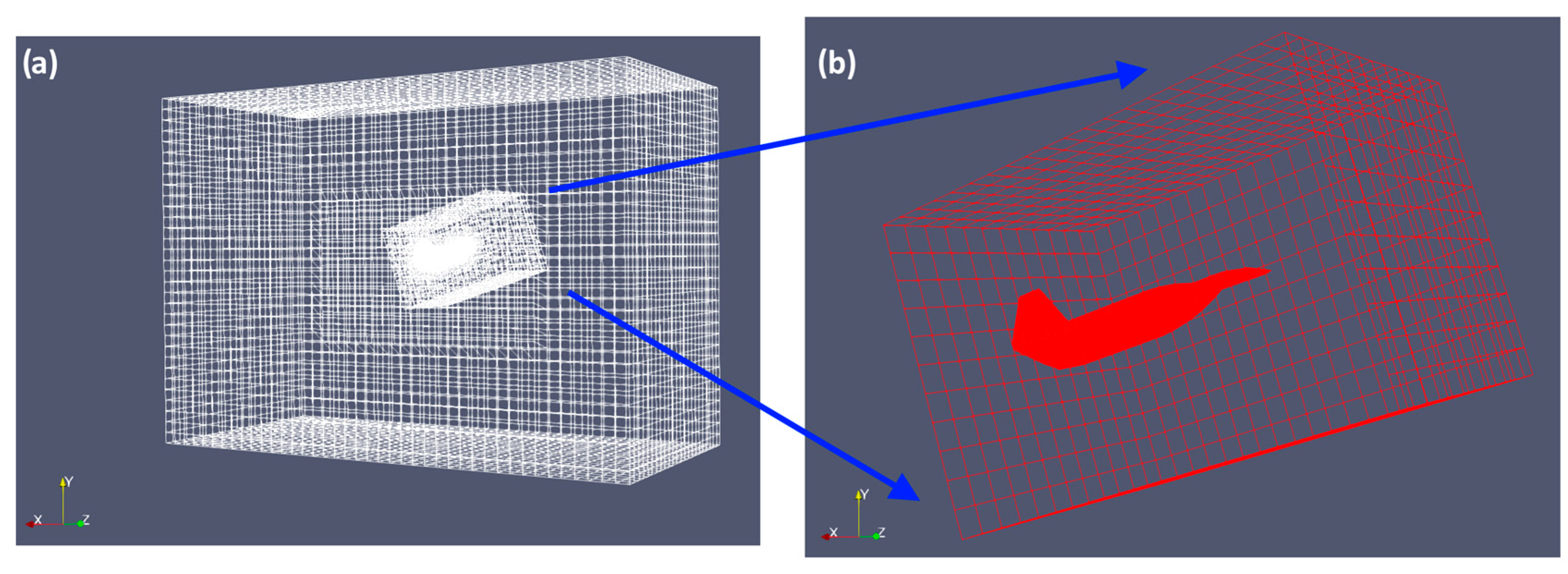
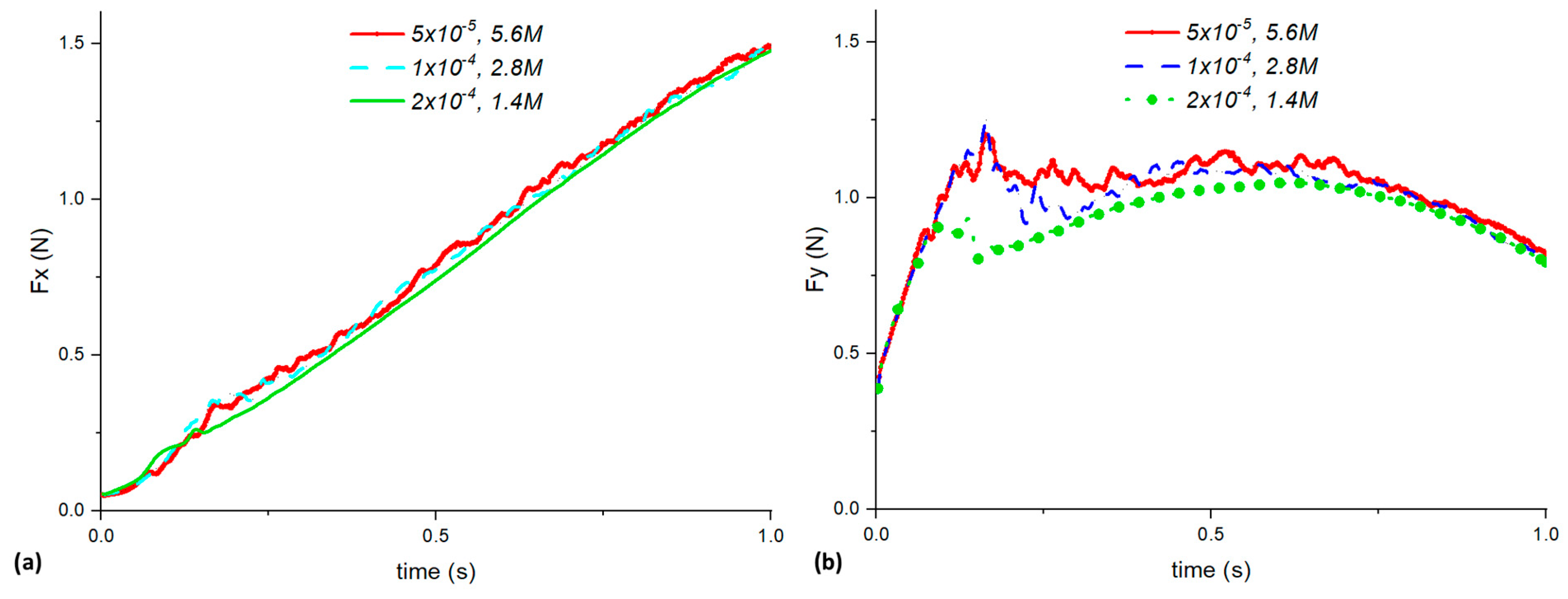
2.3. Grid Convergence Study and Validations

A grid convergence study was performed to find the most suitable grid size for all the simulations. The grid sizes tested were 1.4, 2.8, and 5.6 million cells, with their corresponding distance from the first grid cell to the surface wall at 2 × 10⁻⁴, 1 × 10⁻⁴, and 0.5 × 10⁻⁴ m, respectively. The transient solver pimpleFoam was used to run a simulation involving the UAV performing a prescribed pitch-up maneuver at 1 rad/s. As the aim of this convergence study was to select a suitable grid size, we did not want to involve 6DOF simulations with the new MG6DOFM. The MG6DOFM will be validated in the next section with experiments. Results from Figure 3 show that a grid size of 2.8 M can give a reasonably accurate simulation. Hence, this grid size will be used for all the subsequent simulations in this study.

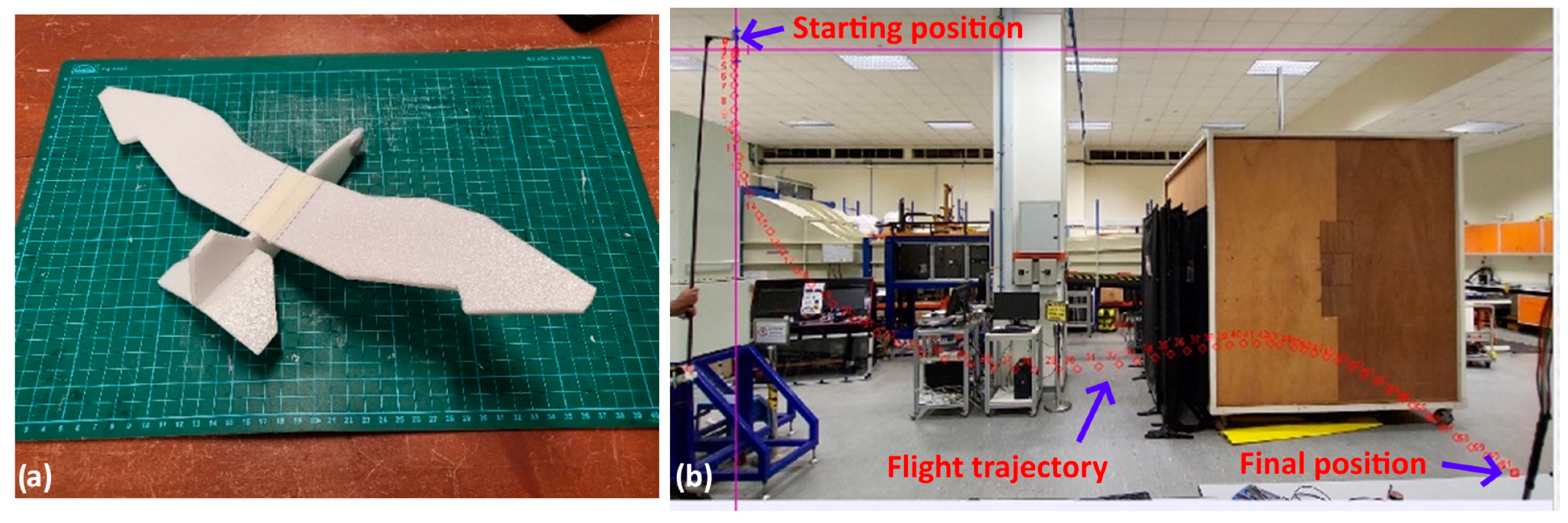
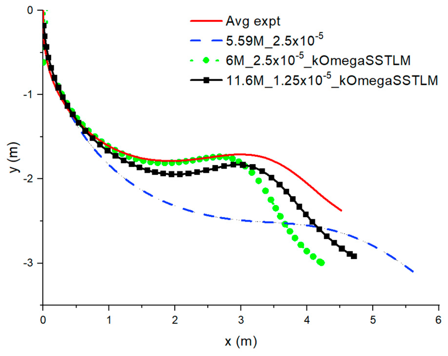
2.4. Experimental Validation of the MG6DOFM Solver

The MG6DOFM code was validated using a free fall experiment with a model aircraft. The model aircraft and the free fall experimental setup are shown in Figure 4. The foam model, which was based on a bird-inspired UAV, had a wing root chord of 0.058 m and a wingspan of 0.403 m, with the fuselage being 0.185 m in length. The free fall experimental setup consisted of a base and an adjustable rod to bring/raise the model to a height of 3 m and an arm with a gripper attached to its end to hold the model in place. When the gripper opens, the model begins to fall. Videos of the model’s trajectory were captured using a smartphone camera at a frame rate of 30 frames per second. The experiment was then repeated five times to account for any differences in the test environment. The trajectory of the model was analyzed using Tracker [16] and then digitized.

For the numerical aspect, the simulation was performed in OpenFOAM with pimpleFoam and the MG6DOFM. The turbulence model used was the Langtry-Menter k-omega Shear Stress Transport (kOmegaSSTLM), which is a transitional turbulence model [17]. The result in Figure 5 shows that we can obtain reasonable agreement with the experimental results. The minor discrepancies in the latter part of the trajectory may be due to inaccuracies in the measurement of elevator angle, moment of inertia, and center of gravity. More details about the experiment and numerical validation can be found in the paper by Tay et al. [18].

3. Research Methodology

As mentioned earlier, the objective of the current study was to design a framework to create a virtual test environment, with the current focus on perch maneuver. We hope to obtain a better understanding of the underlying aerodynamics of the UAV perching maneuver through this virtual environment. To improve the realism of the maneuver, we aimed to replicate the operating conditions as much as possible. As will be shown later, wing deformation alone is insufficient to achieve a good perch landing. Hence, we also added elevator control and emulated propeller lift. These will be discussed in the following sections.

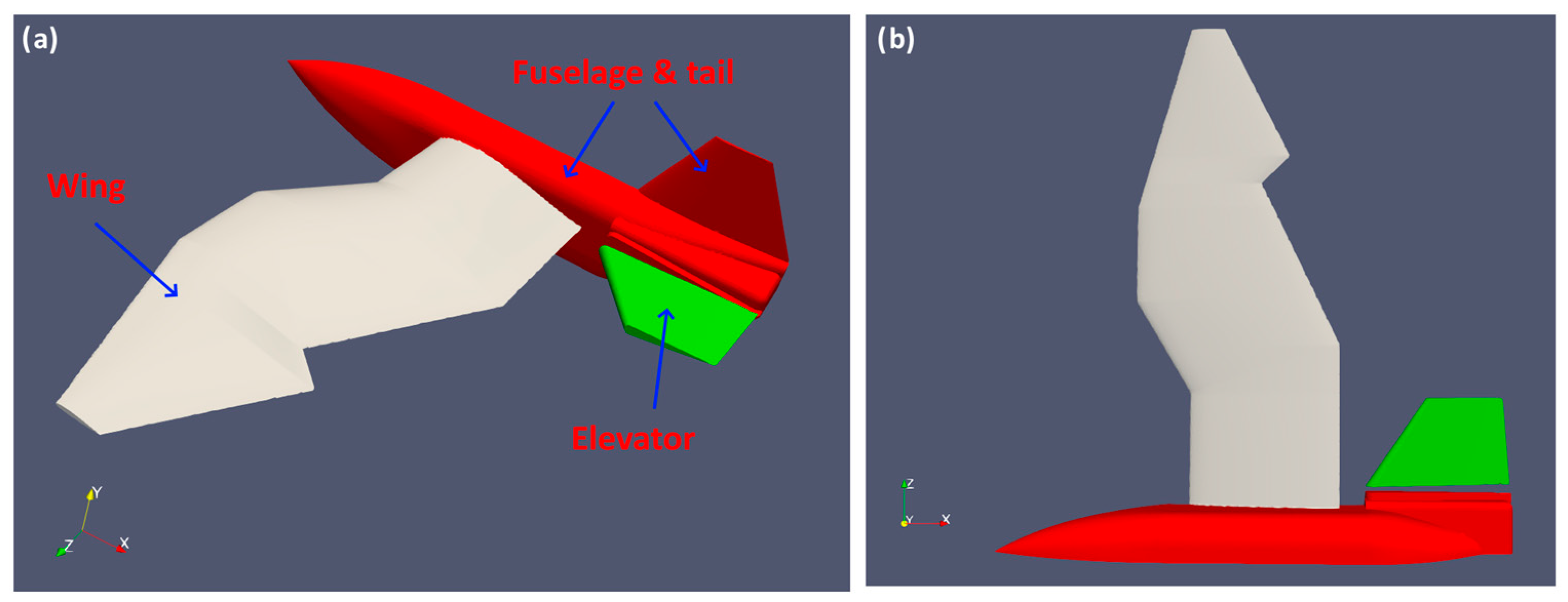
3.1. UAV Prototype and Wing Deformation

The full UAV (wing, fuselage, elevator) was modeled in the simulations, as shown in Figure 6. It was a typical UAV with a wingspan of 1.5 m. As shown in Figure 7 on the left, the UAV was in a neutral wing position during forward flight. However, its wings deformed to a “retract forward” position on the right figure to allow it to perform a perching maneuver by pitching up in flight and landing shortly after. The vertical distance of the UAV above ground was designed at 2.5 m, and the simulation for each case ran for a maximum of 3 s, or shorter if it reached ground before that.

As shown in Figure 7, the green-outlined region of the wing does not deform, while the red-outlined region only translates. The yellow outlined region is the portion that rotates, and the total rotation is 22.5 deg. In the first set of simulations, we investigated the effect of the rate of wing deformation, from 45 deg to 135 deg/s, as compared to the non-deformed case. The upper limit of 135 deg/s was based on the maximum feasible actual servo rotation speed found in the market. These different cases, as given in

Table 1. Different types of cases simulated according to the wing deformation speed.

Cases	1	2	3	4
Wing deformation speed (deg/s)	0 (non-deforming)	45	90	135

, allowed us to compare the differences in the aerodynamic performance of the UAV.

3.2. Elevator Control

In an aircraft, the function of the elevator is to control its pitch angle, and it is an important component in the perch landing maneuver. Hence, in the second set of simulations, we added the functionality of the elevator and compared it with the previous results. As shown in Figure 8, deflecting up the elevator causes the UAV to pitch up. Together with the deforming wing, this enables the UAV to pitch up with a higher angle of attack (AoA) and maintain this position longer to create more drag force.

The elevator is initially at AoA = 0°, and it rotates counterclockwise to help with the pitching up of the UAV. In this study, we designed the elevator’s rotational motion with a simple feedback algorithm, which is given by the following pseudocode:

Pseudocode for elevator’s rotational motion with a simple feedback algorithm
	omega of elevator = -feedback_coeff × (desired_pitch_angle_ − saved_pitch)
	angle_ = angle_old_ + omega of elevator × delta_t,

where the following is true:

saved_pitch is the current pitch angle of the UAV;

desired_pitch_angle is the pitch angle we would like the UAV to maintain;

feedback_coeff is a coefficient to control the rate of increase of omega;

angle_old is the pitch angle from the previous time step.

In this way, the angle of the elevator will be rotated to try to maintain the pitch angle of the UAV. The value of omega is also limited by max_omega, which is the fastest possible rotation speed. This is to ensure that the rotation speed is realistic.

3.3. Emulated Propeller Lift

In the third set of simulations, we provided another way to maintain the UAV’s pitch angle, which was to provide additional lift in the upward direction. This additional lift was used to provide drag to help in the landing instead of increasing the altitude of the UAV. In aeromodeling, the pilot can use the propeller of the plane to provide this lift. However, due to the direction of the propeller, it will also provide a small amount of forward thrust due to thrust vectoring. The idea is that the overall drag created by the UAV’s pitch angle is still larger with the help of the propeller.

Hence, in the 6DOF simulations, we added this emulated propeller lift. The pseudocode is given by the following:

Pseudocode for emulated propeller lift with a simple feedback algorithm
	if t < activation_time then
		propeller_lift = 0
		propeller_lift_x = 0
		propeller_lift_y = 0
	else
		propeller_lift_y = (t − activation_time) × (t − activation_time) × propeller_coeff
		propeller_lift = propeller_lift_y/abs(sin(angle_old))
		if (propeller_lift > max_propeller_lift_) then
			propeller_lift = max_propeller_lift
		propeller_lift_x = propeller_lift × cos(-angle_old)
		propeller_lift_y = propeller_lift × abs(sin(angle_old))

In the pseudocode, the emulated propeller lift is only activated after activation_time t_act, and it increases quadratically after that. Propeller_lift_x and propeller_lift_y are the propeller_lift in the x and y directions. Max_propeller_lift is the maximum possible propeller lift, which in this study is given as 6.867 N, equivalent to about 95% of half the weight of the UAV. The propeller_coeff is similar in function to the previously mentioned feedback_coeff, which is a coefficient used to control the rate of the increase in propeller lift. We investigated the effect of three different activation times (t_act = 0, 0.5 and 1 s) on the landing maneuver.

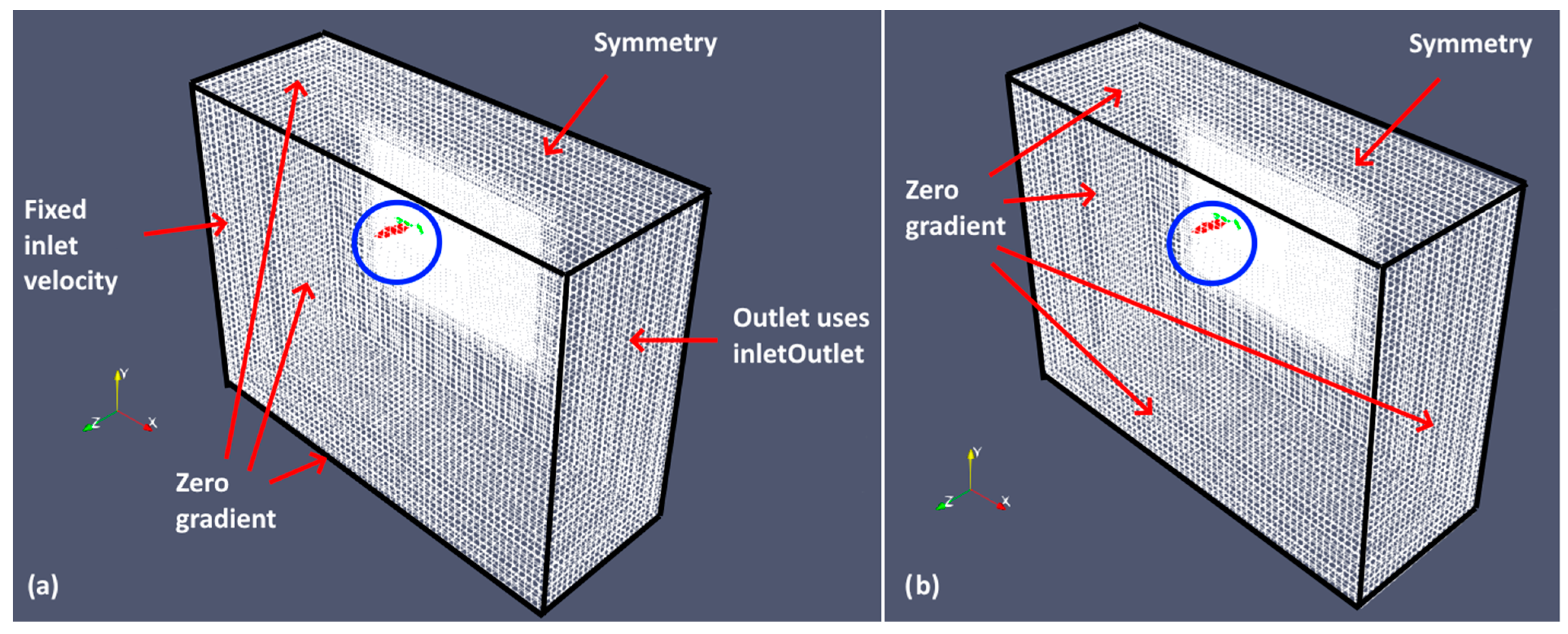
3.4. Simulation Setup

Due to the symmetry of the problem, we only modeled half of the full UAV to save computational resources. The UAV was assumed to fly at a typical speed of 50 km/h, which translates to 13.89 m/s. With a chord of 0.194 m, the Reynolds number (Re) for this study was approximately 172,000. The flow was assumed to be fully turbulent, and the kOmegaSST turbulence model was used in the simulation. The weight of the half UAV was 0.75 kg. The moment of inertia about its center of gravity was (0.013, 0.0362, 0.0246) kg.m², estimated using Solidworks. Hence, the pitching moment of inertia was 0.0362 kg.m². The grid size used was 2.8 M for the simulations without elevator rotation. With the elevator rotation included, AMI had to be used, which increased the grid size to 3.4 M. A distance from the first grid cell to the surface wall of 1 × 10⁻⁴ m was used, corresponding to a y+ of 5. The domain size was 7.7 × 6 × 2.8 m, with the fuselage along the x direction and the symmetry condition applied along the z axis.

In this part of the initial study, an unsteady static simulation using OpenFOAM pimpleFoam, with the wing at an AoA of 6.5 deg in the neutral position, was first performed. This was to ensure that the lift force was sufficient to balance the weight and that the pitching moment M_z was small so that there was pitch stability in the current configuration. In this case, the velocity boundary conditions are given in Figure 9a. The inletOutlet is a boundary condition in OpenFOAM, which gives a zero gradient boundary or zero fixed value depending on the flux going out or into the domain, respectively. The average forces and moments are given in

Table 2. Average forces and moments simulated using OpenFOAM’s pimpleFoam.

Fx (N)	Fy (N)	Mz (Nm)
0.90	7.50	0.0064

. A second moving grid simulation was performed for 2 s. The UAV was prescribed to move with a constant velocity of 13.89 m/s. The boundary conditions are given in Figure 9b. This was to ensure that the flow field was well developed, and the flow field results were used as initial conditions for the subsequent 6DOF moving grid simulations. For both static and moving grid simulations, zero pressure gradient was given for all sides of the domain.

There were, in total, three sets of 6DOF simulations, each focusing on a different objective. At the start of these simulations, the UAV started its descent with its forward thrust switched off. As mentioned in the first set, the wing of the UAV was made to deform at different prescribed rates. The elevator was fixed, and there was no emulated propeller lift. As the simulation proceeded, the UAV pitched and translated in the vertical and horizontal directions due to the action of the forces and moments. In the second set of simulations, the rotation of the elevator came into play, and we observed how this affects the trajectory of the UAV. In the last set of simulations, we added in the effect of emulated propeller lift in addition to wing deformation and elevator rotation. Different activation times were investigated to determine how the landing maneuver is affected. All simulations run up to a maximum of 3 s, or shorter if it reaches ground first (2.5 m below starting altitude)

4. Results and Discussions

In this section, we will present our results for the cases mentioned earlier.

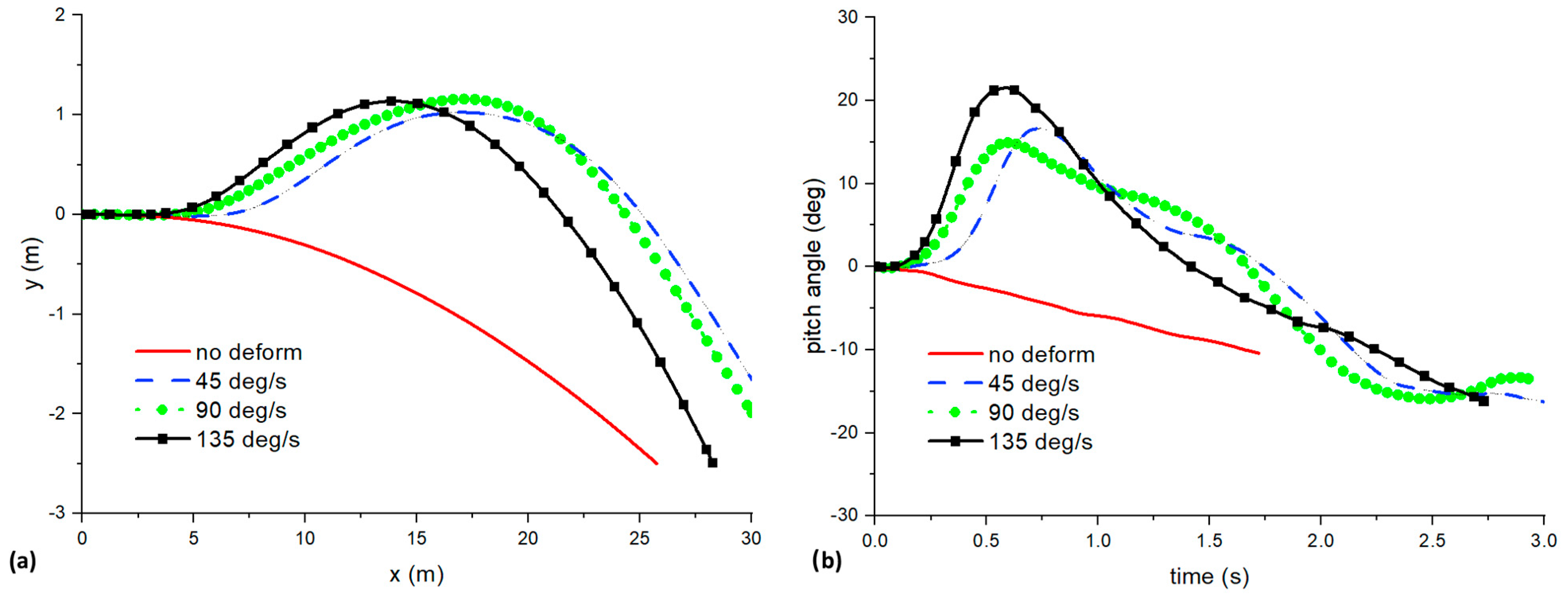
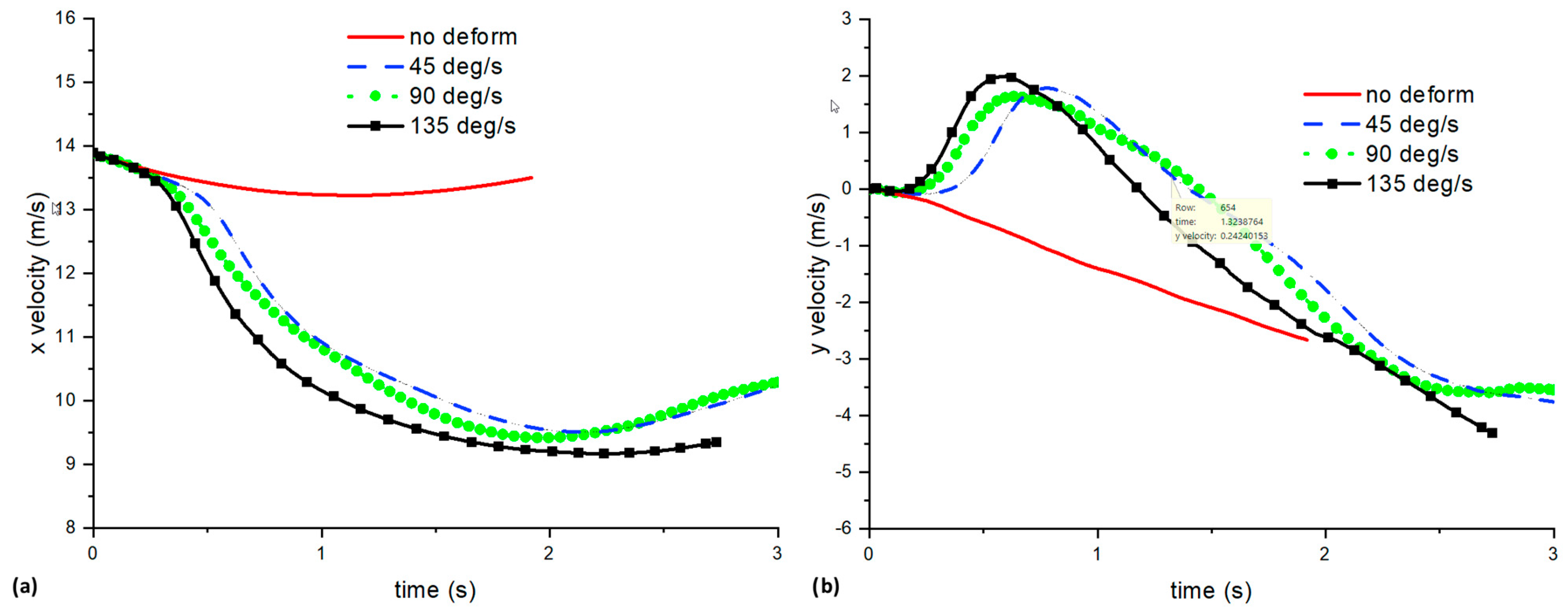
4.1. Pure Wing Deformation Results

In this study, we considered 3DOF, namely pitch and horizontal (x-axis) and vertical translations (y-axis). From the simulations, we could obtain various important information. These include the following:

(1)

velocity/pressure flow fields;

(2)

x/y displacement, velocity, and acceleration;

(3)

pitch angle and angular velocity of the UAV.

Figure 10 shows the plot of delta y against delta x and pitch angle against time for different wing deformations. Without any deformation, we observe that the UAV simply reduces its vertical height y. However, for cases with wing deformation, due to the shift in the center of gravity (CG), they pitch up and increase in altitude first, stall, and descend. This trajectory is similar to the perch landing maneuver seen in birds. However, birds are able to do it in a much sharper and faster fashion, with a pitch angle close to 90 deg, as discussed in the paper by Chin and Lentink [19]. As the speed of wing retraction increases from 45 to 135 deg/s, the UAV tends to pitch up faster and increases its altitude faster. However, the maximum altitude is the same, no matter how fast the retraction speed is. Similarly, the pitch angle plot paints a similar picture. With wing deformation, the UAV can attain a maximum pitch angle of 22 deg.

Figure 11 shows the combined snapshots of the 45 deg/s case from t = 0 to 2.8 s, with a lapse of 0.4 s per image. Its corresponding drag F_x and lift F_y variations against time are given in Figure 12. One can observe that as the wing deforms and retracts forward, it pitches up due to the positive pitch (assuming that clockwise is positive). This increases the lift generated by the wings, and the UAV increases its altitude. However, as the pitch angle continues to increase, stall starts to set in and lift and drag start to decrease and increase, respectively. There is a slight lag between the variation of lift and drag. The UAV then begins to decrease its altitude and pitch down rapidly due to a pitching-down moment. As the AoA decreases, drag decreases too. Figure 13 shows a close-up view of the wing deforming and retracting, with the contour showing the change in pressure within the 0.6 s time frame. Between t = 0.4 and 0.6 s, we can observe the large pressure change. For this 45 deg/s case, it takes 0.5 s to finish the wing retracting motion.

For landing, one of the important considerations is the velocity just before landing. Figure 14 shows the plot of horizontal (x) and vertical (y) velocity against time for the various retract motions subjected to a landing height of 2.5 m. The x velocity of the UAV without deformation slows down slightly before increasing its speed just before landing. A speed of 14 m/s is simply too fast for landing. The UAV without deformation had a y velocity of −3 m/s. On the other hand, for the UAVs with wing deformation, their x velocity lay in the range of 9 and 11 m/s. This is about 32% slower than the non-deformed wing case, although still reasonably fast. In terms of y velocity, there was an increase in magnitude from 2.6 to between 3.5 and 4.5 m/s. This is because the deformed wing cases pitch up and gain altitude before diving down. Of the three retraction speeds, the 135 deg/s case had a slightly lower landing x velocity, although it also had a slightly faster landing y velocity.

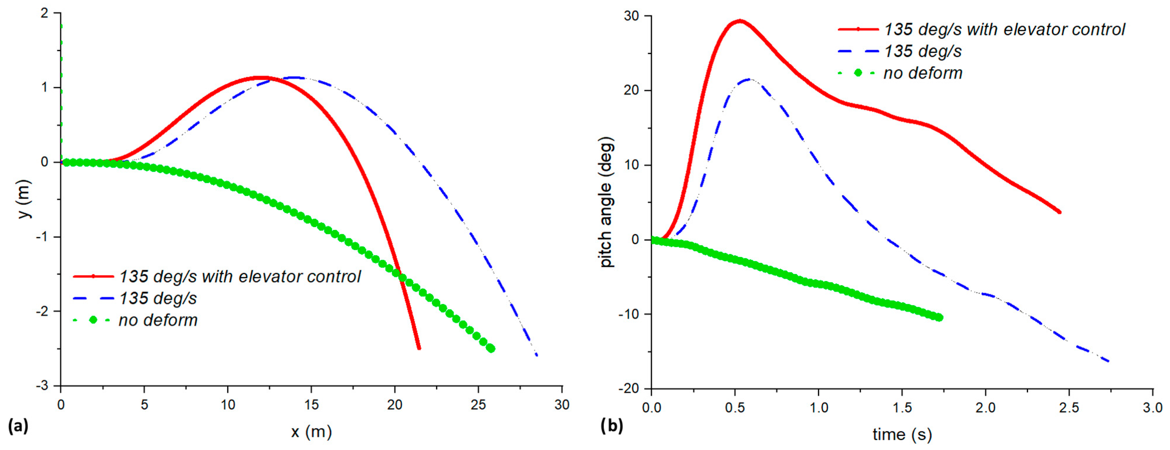
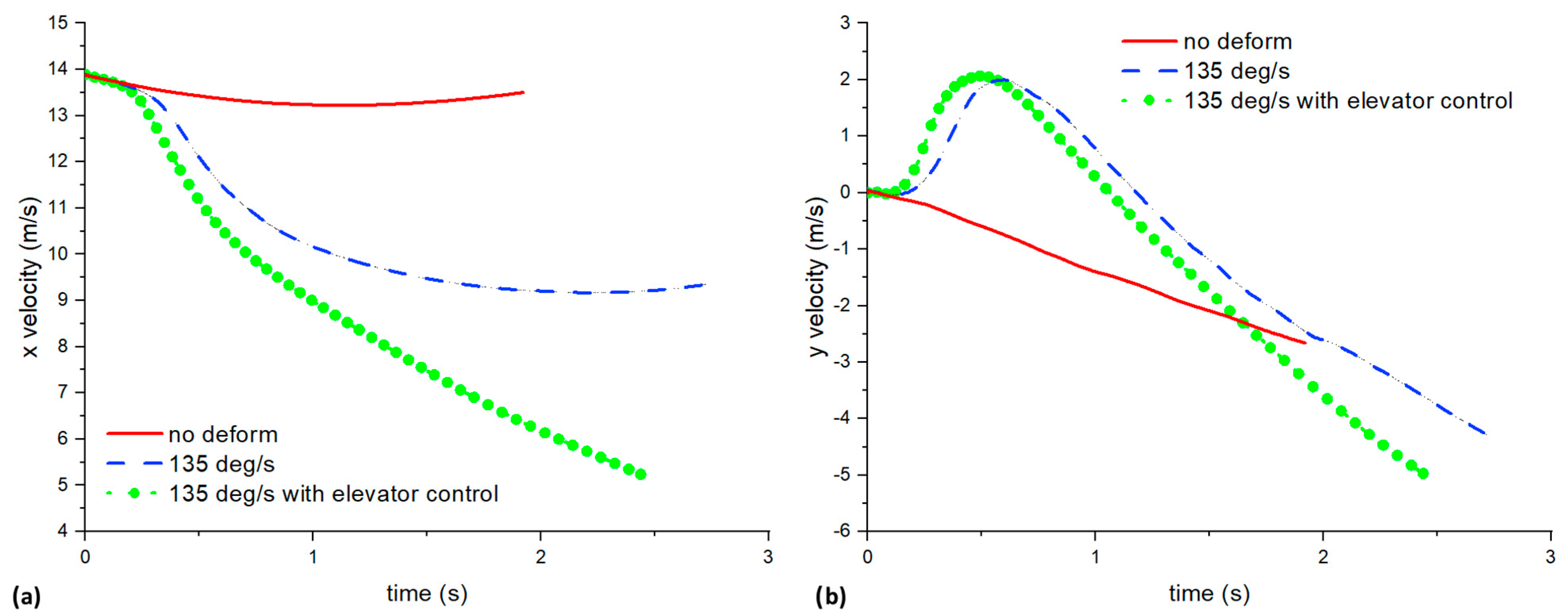
4.2. Wing Deformation with Elevator Control

In this case, we added elevator control. The wing deformation was fixed at 135 deg/s. Figure 15 shows the (a) trajectory and (b) pitch angle of the UAV for the non-deformed, pure deformed, and with additional elevator control cases. As shown in Figure 15a, the UAV with elevator control has similar altitude gain compared with the purely deformed case, but it has a much sharper descent, resulting in a shorter x displacement. This is advantageous for landing, as the ground clearance required is less. This result shows that the elevator can effectively reduce the landing distance. It must also be noted that the algorithm used to control the elevator is rather simple. Moreover, the pitch angle of the deformed case with elevator control is also higher than the pure deformed case (30 deg against 20 deg), which creates more forward drag and reduces the landing distance. Hence, with this 6DOF simulation framework, we can visualize and predict different information, just like in an actual flight test. Some of this information obtained from the simulations may not be available in an actual flight test due to the lack of certain hardware.

Figure 16 shows the comparison of x/y velocities of non-deformed, pure deformed, and deformation with elevator control cases. The UAV with elevator control managed to reduce its x velocity to around 5 m/s, which is even lower than the pure deformed case of around 9 m/s. This result shows that the elevator greatly helps to reduce landing speed and displacement. With CFD, we can also visualize the flow fields to obtain a better understanding of the aerodynamics. Figure 17 shows the vorticity at the z = 0.4 m slice and surface pressure on the deforming wing with elevator control during the pitch-up maneuver from t = 0 to 1.5 s. As the wing deformed, the UAV pitched up, and it created a leading-edge vortex (LEV). At t = 0.6 s, the UAV’s pitch angle reached its maximum. The LEV remains attached, and the trailing-edge vortex (TEV) starts to appear as well. LEV is an important component of unsteady flight, especially in flapping-wing flight cases, and it can help to create a large lift force [20]. The study by Adhikari et al. [8] also mentions the importance of the stability of the LEV on the lift. We can also observe how the surface pressure of the wing changes throughout the process. Although it was not done here, it is possible to compare and analyze the different perching configurations and visualize the vorticity and pressure contours to see how it is possible to achieve a higher pitch angle or lower forward velocity. This highlights another advantage of using this 6DOF CFD analysis.

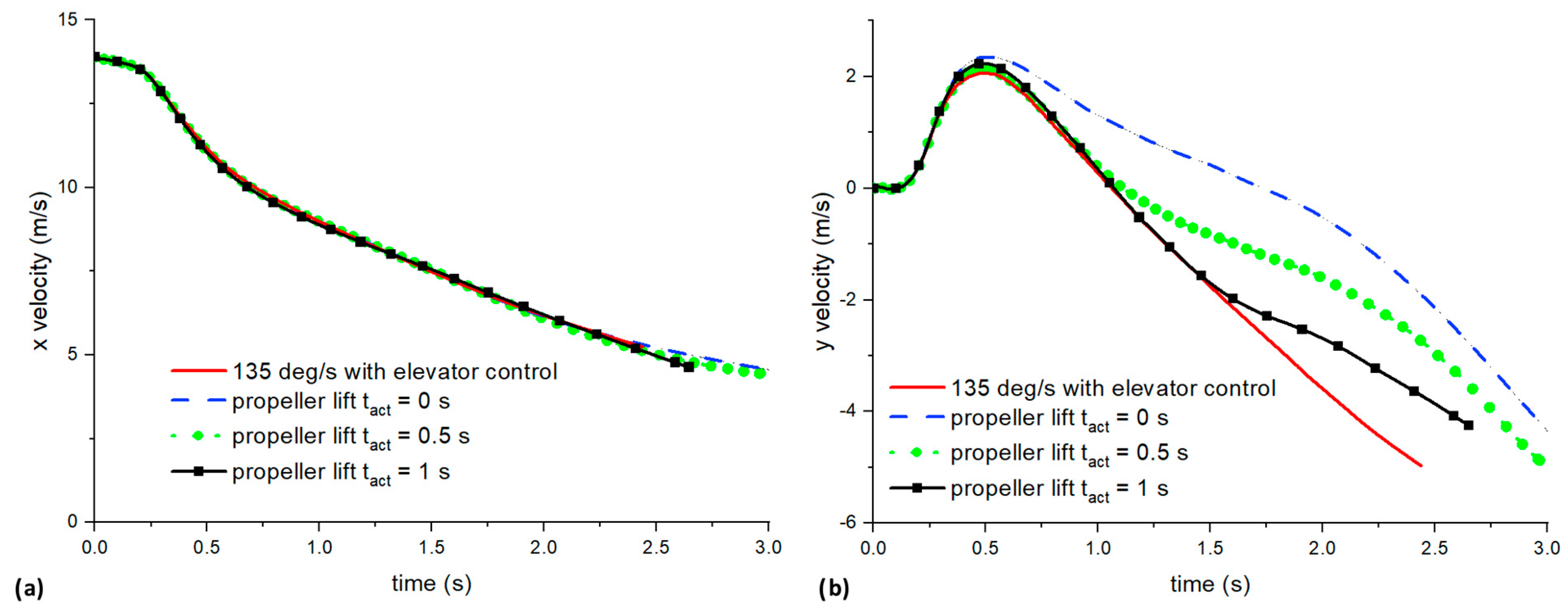
4.3. Wing Deformation with Elevator Control and Emulated Propeller Lift

In this section, besides the wing deformation and elevator control, we added the emulated propeller lift. As shown in Figure 18a, if the propeller lift is activated right at the start, it will cause the altitude of the UAV to increase much higher compared with the rest, which is not desirable, as the objective is to land as fast as possible. In fact, after 3 s, the UAV was still at a height of −0.5 m, 2 m away from the landing height. There was almost no difference in maximum altitude when the propeller lift was activated at t_act = 0.5 and 1 s. In comparison, the maximum pitch angle of the UAV was almost the same (~ 30 deg), although the decrease in pitch angle as time progresses is slower for cases with propeller lift. This is because the propeller lift provided an upward force to maintain the pitch angle.

Figure 19 shows the comparison of x/y velocities against time for elevator and emulated propeller cases for all cases. There was almost no difference in the decrease of x velocity between the different cases, except that for cases with propeller lift, the x velocity at landing was slightly lower (4.4 against 5.2 m/s). This was still beneficial for landing. In terms of y velocity, for cases with propeller lift at t = 0 and 1 s, their y velocity magnitude at landing was relatively smaller (4.2/4.3 against 4.9/5 m/s) than the other two cases. These results show that propeller lift can help to reduce the landing x and y velocities by a small margin. The algorithm used for the propeller lift is relatively simple, and hence, a better algorithm, such as the use of deep reinforced learning [3], may be able to give a better performance.

5. Conclusions and Future Works

The perching maneuver of a wing-deforming UAV was investigated using the free, open-source solver OpenFOAM through the 6DOF framework. This framework can perform 6DOF moving grid simulations together with grid deformation, sliding mesh, and algorithm addition capabilities. With the moving grid capability, one can save substantially on computational resources. Results show that when the wing retracts forward, the UAV pitches up and slows down. From the 6DOF analysis, we can analyze the trajectory of the UAV. The different retraction speeds have slightly different effects on the trajectory of the UAV. It was found that a retraction speed of 135 deg/s allows the UAV to have a slightly lower landing x velocity and a higher landing y velocity. Although the forward speed of the wing-deformed UAV decreases by 32%, it is still too fast for landing. With the addition of the elevator, the x velocity can be decreased to 5 m/s, with the y velocity magnitude maintained at 5 m/s. This shows the effectiveness of the elevator control. Lastly, we added the emulated propeller lift. If the emulated propeller lift is activated at the start of the wing deformation, its altitude will increase too high and too fast. In comparison, if the lift is activated 0.5 to 1 s later, it can further help to reduce its landing velocity by a small margin. Better performance may be possible with a better-emulated propeller lift algorithm. In this study, the focus was on the perch landing maneuver. The results show that this framework can be used for the accurate prediction of the trajectory of UAVs with fixed or movable wings and control surfaces. It is also possible to add external forces like the emulated propeller lift. The moving grid feature can reduce the computational cost, and together with the free, open-source CFD code OpenFOAM, this can be a viable option compared with other commercial CFD codes, which are more expensive. Moreover, the flexibility of the framework with OpenFOAM means that it can also be used on other problems, such as fast-turning agile flight and flapping wing flight.

References

1. Moore, J.; Cory, R.; Tedrake, R. Robust Post-Stall Perching with a Simple Fixed-Wing Glider Using LQR-Trees. Bioinspir. Biomim. 2014, 9, 025013. [Google Scholar] [CrossRef] [PubMed]
2. Paranjape, A.; Kim, J.; Gandhi, N.; Chung, S.-J. Experimental Demonstration of Perching by an Articulated Wing MAV. In Proceedings of the AIAA Guidance, Navigation, and Control Conference, Portland, OR, USA, 8–11 August 2011. [Google Scholar] [CrossRef]
3. Waldock, A.; Greatwood, C.; Salama, F.; Richardson, T. Learning to Perform a Perched Landing on the Ground Using Deep Reinforcement Learning. J. Intell. Robot. Syst. 2018, 92, 685–704. [Google Scholar] [CrossRef]
4. Wickenheiser, A.M.; Garcia, E. Longitudinal Dynamics of a Perching Aircraft. J. Aircr. 2006, 43, 1386–1392. [Google Scholar] [CrossRef]
5. Li, H.; Li, Y.; Zhao, Z.; Wang, X.; Yang, H.; Ma, S. High-Speed Virtual Flight Testing Platform for Performance Evaluation of Pitch Maneuvers. Aerospace 2023, 10, 962. [Google Scholar] [CrossRef]
6. Lukić, N.; Ivanov, T.; Svorcan, J.; Simonović, A. Numerical Investigation and Optimization of a Morphing Airfoil Designed for Lower Reynolds Number. Aerospace 2024, 11, 252. [Google Scholar] [CrossRef]
7. Cheng, B.; Guo, Z. Study on Small UAVs’ Deep Stall Landing Procedure. In Proceedings of the 2017 5th International Conference on Mechanical, Automotive and Materials Engineering (CMAME), Guangzhou, China, 1–3 August 2017. [Google Scholar] [CrossRef]
8. Adhikari, D.R.; Loubimov, G.; Kinzel, M.P.; Bhattacharya, S. Effect of Wing Sweep on a Perching Maneuver. Phys. Rev. Fluids 2022, 7, 044702. [Google Scholar] [CrossRef]
9. Tay, W.B.; Chan, W. Numerical 6DOF Simulation of a Perching Wing Deforming UAV. In Proceedings of the AIAA SCITECH 2023 Forum, National Harbor, MD, USA/Online, 23–27 January 2023. [Google Scholar] [CrossRef]
10. Weller, H.G.; Tabor, G.; Jasak, H.; Fureby, C. A Tensorial Approach to Computational Continuum Mechanics Using Object-Oriented Techniques. Comput. Phys. 1998, 12, 620. [Google Scholar] [CrossRef]
11. Issa, R.I. Solution of the Implicitly Discretised Fluid Flow Equations by Operator-Splitting. J. Comput. Phys. 1986, 62, 40–65. [Google Scholar] [CrossRef]
12. Patankar, S.V.; Spalding, D.B. A Calculation Procedure For Heat, Mass And Momentum Transfer In Three-Dimensional Parabolic Flows. Int. J. Heat Mass Transf. 1972, 15, 1787–1806. [Google Scholar] [CrossRef]
13. Petersson, N.A. Hole-Cutting for Three-Dimensional Overlapping Grids. SIAM J. Sci. Comput. 1999, 21, 646–665. [Google Scholar] [CrossRef]
14. Mittal, R.; Iaccarino, G. Immersed Boundary Methods. Annu. Rev. Fluid Mech. 2005, 37, 239–261. [Google Scholar] [CrossRef]
15. Schnepf, C.; Richter, K. Investigation of the Transient Aerodynamic Behavior of a UAV with Folding Wings in a Generic Airdrop. In Proceedings of the AIAA SCITECH 2024 Forum, Orlando, FL, USA, 8–12 January 2024. [Google Scholar] [CrossRef]
16. Brown, D. Tracker; Cabrillo College: Aptos, CA, USA, 2023. [Google Scholar]
17. Langtry, R.B.; Menter, F.R. Correlation-Based Transition Modeling for Unstructured Parallelized Computational Fluid Dynamics Codes. AIAA J. 2009, 47, 2894–2906. [Google Scholar] [CrossRef]
18. Tay, W.B.; Chong, R.O.; Tay, J.C.M. Numerical Validation and Sensitivity Tests of a Model Aircraft in Free Fall. In Proceedings of the AIAA SCITECH 2024 Forum, Orlando, FL, USA, 8–12 January 2024. [Google Scholar] [CrossRef]
19. Chin, D.D.; Lentink, D. Birds Repurpose the Role of Drag and Lift to Take off and Land. Nat. Commun. 2019, 10, 5354. [Google Scholar] [CrossRef] [PubMed]
20. Ellington, C.P. The Aerodynamics of Flapping Animal Flight. Am. Zool. 1984, 24, 95–105. [Google Scholar] [CrossRef]
Figure 1. A UAV undergoing an ideal perch landing.
Aerospace 11 00657 g001
Figure 2. (a) Overall domain and (b) magnified overset grid.
Aerospace 11 00657 g002
Figure 3. Force (a) Fx and (b) Fy against time plot for the pitch-up maneuver.
Aerospace 11 00657 g003
Figure 4. (a) Model aircraft and the (b) free fall experimental setup.
Aerospace 11 00657 g004
Figure 5. Trajectory plots of y against x for the experiment, numerical laminar, and kOmegaSSTLM results.
Aerospace 11 00657 g005
Figure 6. (a) Isometric and (b) top view of the modeled UAV.
Aerospace 11 00657 g006
Figure 7. (a) Wing in neutral and (b) retract forward positions.
Aerospace 11 00657 g007
Figure 8. Diagram of the elevator.
Aerospace 11 00657 g008
Figure 9. Velocity boundary conditions for the (a) static and (b) moving grid simulations. The blue-circled region indicates the UAV position.
Aerospace 11 00657 g009
Figure 10. Plot of (a) y against x and (b) pitch angle against time for different wing deformations.
Aerospace 11 00657 g010
Figure 11. Timelapse snapshots of the 45 deg/s case from t = 0 to 2.8 s, with a lapse of 0.4 s per image. The color contours indicate the difference in pressure.
Aerospace 11 00657 g011
Figure 12. Plot of Fx and Fy against time for the 45 deg/s case from t = 0 to 2.8 s.
Aerospace 11 00657 g012
Figure 13. Deformation of the wing from t = 0 to 0.6 s.
Aerospace 11 00657 g013
Figure 14. Plot of (a) x and (b) y velocity against time for the various retract motions.
Aerospace 11 00657 g014
Figure 15. Comparison of (a) trajectories and (b) pitch angle of nonpure deformation and deformation with elevator control cases.
Aerospace 11 00657 g015
Figure 16. Comparison of (a) x and (b) y velocities against time of nonpure deformation and deformation with elevator control cases.
Aerospace 11 00657 g016
Figure 17. Vorticity at z = 0.4 m slice and surface pressure on the deforming wing with elevator control during pitch-up maneuver from t = 0 to 1.5 s.
Aerospace 11 00657 g017
Figure 18. Plot of (a) delta y against delta x and (b) pitch angle against time for elevator and emulated propeller cases.
Aerospace 11 00657 g018
Figure 19. Comparison of (a) x and (b) y velocities against time for elevator and emulated propeller cases.
Aerospace 11 00657 g019