Direct Closed-Loop Control Structure for the Three-Axis Satcom-on-the-Move Antenna


Abstract
:1. Introduction
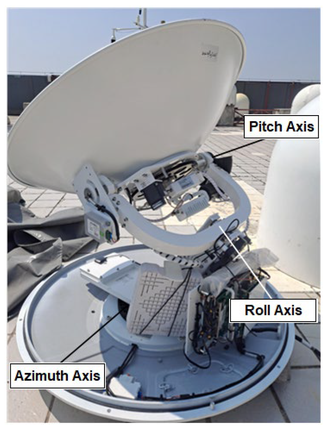
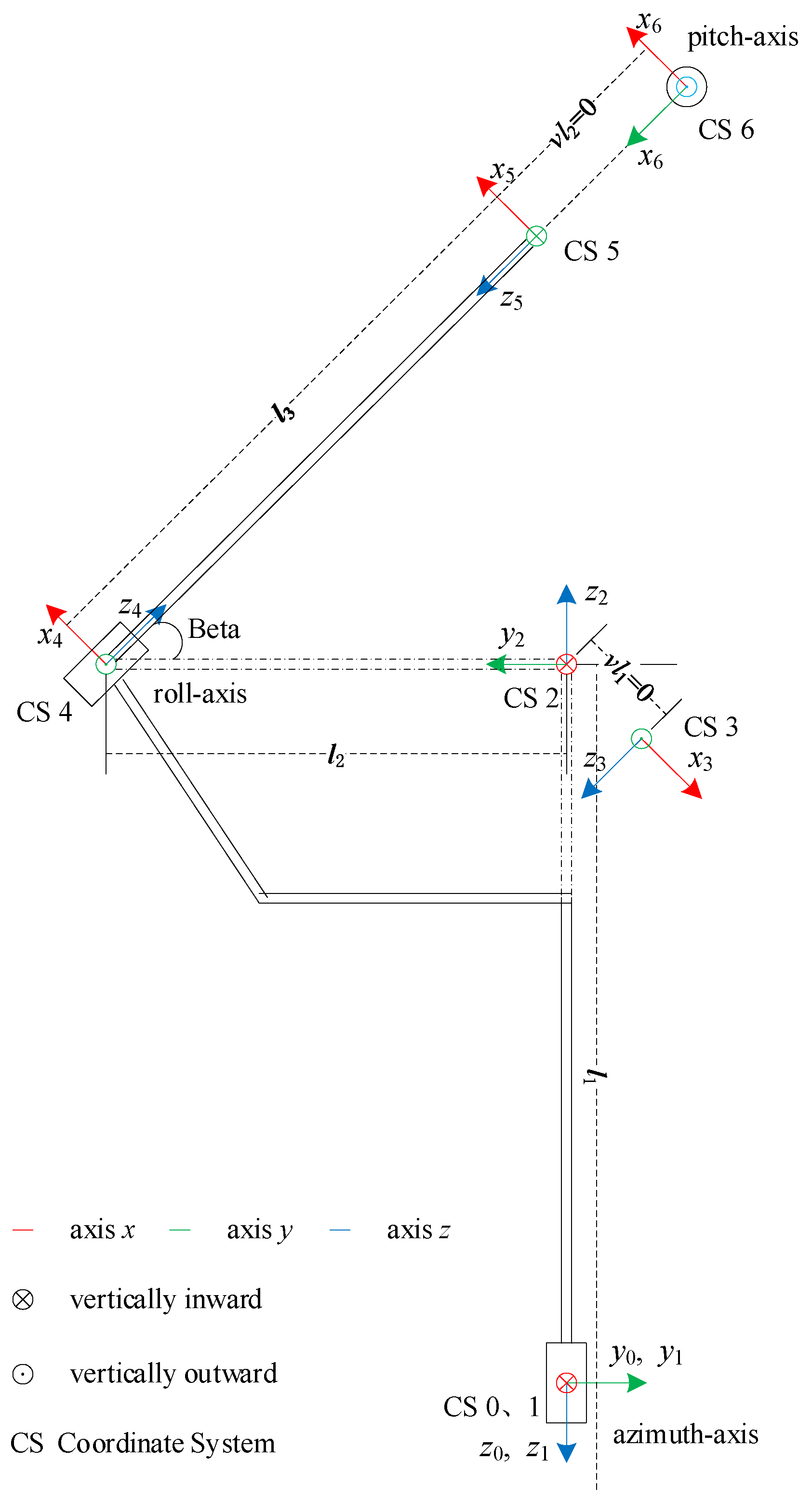
2. The Kinematic Relationship of the Three-Axis SOTM
3. Direct Closed-Loop Control Structure Based on Jacobian Operator
3.1. Jacobian Operator
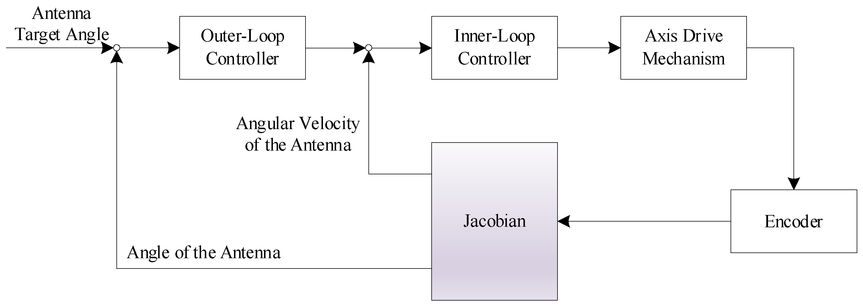
3.2. Direct Closed-Loop Control Structure
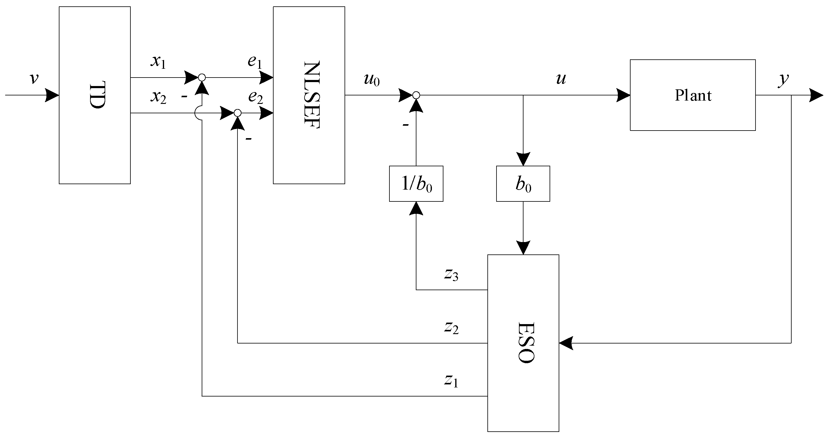
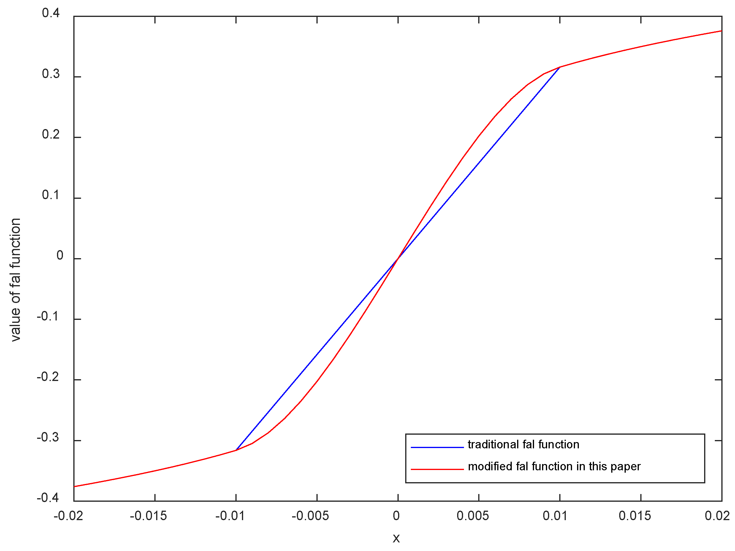
4. Controller Design
5. Experimental Analysis
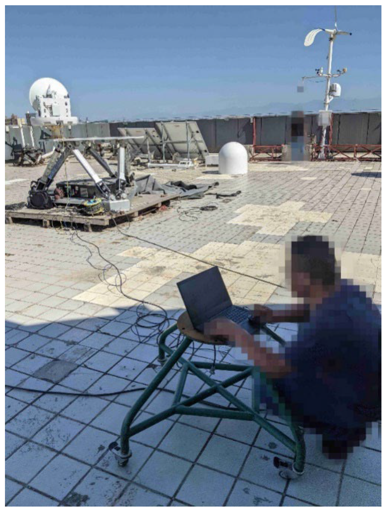
5.1. Experimental Environment
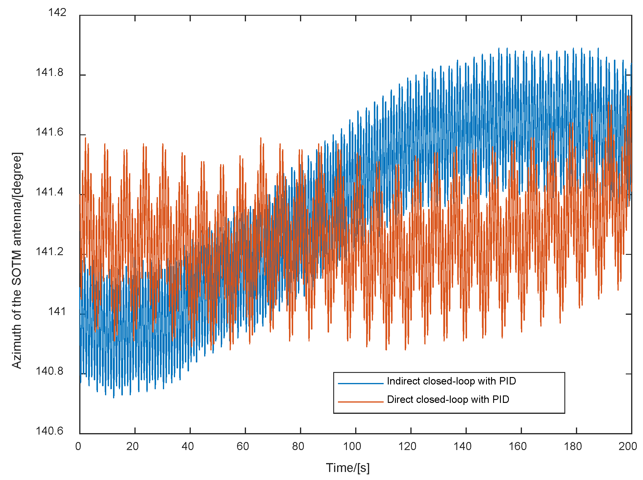
5.2. Experimental Results and Analyses
6. Conclusions
Author Contributions
Funding
Data Availability Statement
Conflicts of Interest
References
- George, A.; Fernando, M.; George, A.; Baskar, T.; Pandey, D. Metaverse: The Next Stage of Human Culture and the Internet. Int. J. Adv. Res. Trends Eng. Technol 2021, 8, 1–10. [Google Scholar]
- Kozyreva, A.; Lewandowsky, S.; Hertwig, R. Citizens Versus the Internet: Confronting Digital Challenges with Cognitive Tools. Psychol. Sci. Publ. Int. 2021, 21, 103–156. [Google Scholar] [CrossRef] [PubMed]
- Shaengchart, Y.; Tanpat, K.; Smich, B. Factors Influencing the Effects of the Starlink Satellite Project on the Internet Service Provider Market in Thailand. Technol. Soc. 2023, 74, 102279. [Google Scholar] [CrossRef]
- Cui, G.; He, Q.; Chen, F.; Jin, H.; Yang, Y. Trading off Between User Coverage and Network Robustness for Edge Server Placement. IEEE Trans. Cloud Comput. 2020, 10, 2178–2189. [Google Scholar] [CrossRef]
- Benavente-Peces, C.; Herrero-Sebastian, I. Worldwide Coverage Mobile Systems for Supra-Smart Cities Communications: Featured Antennas and Design. Smart Cities 2020, 3, 556–584. [Google Scholar] [CrossRef]
- Hassan, N.; Huang, C.; Yuen, C.; Ahmad, A.; Zhang, Y. Dense Small Satellite Networks for Modern Terrestrial Communication Systems: Benefits, Infrastructure, and Technologies. IEEE Wirel. Commun. 2020, 27, 96–103. [Google Scholar] [CrossRef]
- Al-Ahmed, S.; Shakir, M.; Zaidi, S. Optimal 3D UAV Base Station Placement by Considering Autonomous Coverage Hole Detection, Wireless Backhaul and User Demand. J. Commun. Netw. 2020, 22, 467–475. [Google Scholar] [CrossRef]
- Pang, X.; Sheng, M.; Zhao, N.; Tang, J.; Niyato, D.; Wong, K. When UAV Meets IRS: Expanding Air-Ground Networks via Passive Reflection. IEEE Wirel. Commun. 2021, 28, 164–170. [Google Scholar] [CrossRef]
- Li, K.; You, L.; Wang, J.; Gao, X.; Tsinos, C.; Chatzinotas, S.; Ottersten, B. Downlink Transmit Design for Massive MIMO LEO Satellite Communications. IEEE Trans. Commun. 2021, 70, 1014–1028. [Google Scholar] [CrossRef]
- Chen, Z.; Qing, X.; Tang, X.; Liu, W.; Xu, R. Phased Array Metantennas for Satellite Communications. IEEE Commun. Mag. 2020, 60, 46–50. [Google Scholar] [CrossRef]
- Han, L.; Li, G.; Ren, J.; Ji, X. Synthetic Deviation Correction Method for Tracking Satellite of the SOTM Antenna on High Maneuveribility Carriers. Electronics 2022, 11, 3732. [Google Scholar] [CrossRef]
- Gunnar, R.; James, D. Servo requirements for FCC VMES compliance: Servo performance levels required to meet FCC VMES pointing requirements for satcom-on-the-move antennas on ground vehicles. In Proceedings of the 2010 Military Communications Conference (2010—MILCOM), San Jose, CA, USA, 31 October–3 November 2010. [Google Scholar]
- Alazab, M.; Felber, W.; Galdo, G.; Heuberger, A.; Lorenz, M.; Mehnert, M.; Raschke, F.; Siegert, G.; Landmann, M. Pointing Accuracy Evaluation of SOTM Terminals under Realistic Conditions. In Proceedings of the 34th ESA Antenna Workshop on Challenges for Space Antenna Systems, Noordwijk, The Netherlands, 3–5 October 2012. [Google Scholar]
- Hancıoğlu, O.; Mehmet, Ö. Neural Network Control of a SOTM Antenna. In Proceedings of the 2023 9th International Conference on Control, Decision and Information Technologies (CoDIT), Rome, Italy, 3–6 July 2023. [Google Scholar]
- Michal, B.; Jan, N.; Tomas, S. Design of an Antenna Pedestal Stabilization Controller Based on Cascade Topology. In Proceedings of the Mechatronics 2019: Recent Advances Towards Industry 4.0, Warsaw, Poland, 16–18 September 2019. [Google Scholar]
- Laetitia, T.; Minh, P.; Paolo, M.; Elliot, B. Rapid Transfer Alignment for Large and Time-Varying Attitude Misalignment Angles. IEEE Control Syst. Lett. 2023, 7, 1981–1986. [Google Scholar]
- Ren, J.; Ji, X.; Han, L.; Li, J.; Song, S.; Wu, Y. Rapid Tracking Satellite Servo Control for Three-Axis Satcom-on-the-Move Antenna. Aerospace 2024, 11, 345. [Google Scholar] [CrossRef]
- Wang, Y.; Zhang, C.; Zuo, Z. Anti-windup Active Disturbance Rejection Control and its Application to Antenna Servo Systems. In Proceedings of the 2019 Chinese Control Conference (CCC), Guangzhou, China, 27–30 July 2019. [Google Scholar]
- Xue, X.; Zheng, J.; Yuan, D. Adaptive Control of Servo Motor in “SOTM”. In Proceedings of the 2018 3rd International Conference on Control, Automation and Artificial Intelligence (CAAI 2018), Beijing, China, 26–27 August 2018. [Google Scholar]
- Liu, H.; Wang, B.; Zhou, Z.; Pan, D. An Active Disturbance Rejection Controller for Azimuth Speed Control of Mobile SATCOM Flat Antenna. In Proceedings of the 2013 IEEE International Conference on Information and Automation (ICIA), Yinchuan, China, 26–28 August 2013. [Google Scholar]
- Wu, Z.; Yao, M.; Jia, W.; Tian, F. Low-Cost Attitude Estimation Based on MIMU/GPS Integration for SOTM. In Proceedings of the 2012 Second International Conference on Electric Information and Control Engineering, Lushan, China, 6 April 2022. [Google Scholar]
- Galkin, A.; Puzikov, V.; Mikheev, A.; Tulush, A.; Timoshenkov, A. Mobile Satellite Antenna Control System Based on MEMS-IMU. In Proceedings of the 2021 IEEE Conference on Russian Young Researchers in Electrical and Electronic Engineering (EIConRus), Moscow, Russia, 26–29 January 2021. [Google Scholar]
- Liu, J.; Lin, C.; Lo, H. Pseudo-inverse Jacobian Control with Grey Relational Analysis for Robot Manipulators Mounted on Oscillatory Bases. J. Sound Vib. 2009, 326, 421–437. [Google Scholar]
- Connor, W.; Rosario, O.; Tania, M. Closed-Loop Position Control for Growing Robots Via Online Jacobian Corrections. IEEE Robot Autom. Lett. 2021, 6, 6820–6827. [Google Scholar]
- Rodrigo, S.; Rodney, G. A More Compact Expression of Relative Jacobian Based on Individual Manipulator Jacobians. Robot. Auton. Syst. 2015, 63, 158–164. [Google Scholar]
- James, D. Control Systems for Mobile Satcom Antennas. IEEE Control Syst. Mag. 2008, 28, 86–101. [Google Scholar]
- Yang, P.; Guo, Z.; Kong, Y. Plane Kinematic Calibration Method for Industrial Robot Based on Dynamic Measurement of Double Ball Bar. Precis. Eng. 2020, 62, 265–272. [Google Scholar] [CrossRef]
- Wen, X.; Wang, D.; Zhao, Y.; Kang, C.; Zhang, Y.; Lv, Z. A Comparative Study of MDH and Zero Reference Model for Geometric Parameters Calibration to Enhance Robot Accuracy. In Proceedings of the Ninth International Symposium on Precision Mechanical Measurements, Chongqing, China, 18–21 October 2019. [Google Scholar]
- Diao, S.; Chen, X.; Luo, J. Development and Experimental Evaluation of a 3D Vision System for Grinding Robot. Sensors 2018, 18, 3078. [Google Scholar] [CrossRef] [PubMed]
- Ren, J.; Ji, X.; Li, J.; Han, L.; Wu, Y. A Kinematic Modeling Scheme of Three-Axis” Satcom-on-the-Move” Antenna Based on Modified Denavit-Hartenberg Method. J. Northwest. Polytech. Univ. 2023, 41, 518–528. [Google Scholar] [CrossRef]
- John, C. Introduction to Robotics Mechanics and Control, 4th ed.; Pearson Education: London, UK, 2017; pp. 157–158. [Google Scholar]
- Liu, X.; Qin, C. Disturbance Observation and Compensation Design of SOTM Antenna. J. Chongqing Univ. Technol. Nat. Sci. 2023, 37, 129–134. [Google Scholar]
- Ren, J.; Ji, X.; Li, J.; Han, L.; Wu, Y. Distributed Dynamic Backup Servo Control for Satcom-on-the-Move Systems. In Proceedings of the 14th Asia Conference on Mechanical and Aerospace Engineering, Hong Kong, China, 22–24 December 2023. [Google Scholar]
- Gao, W.; Zhang, M.; Lu, G.; Gao, H. Design of Position Loop of On-the-Move Servo System Based on Fuzzy Control. Ship Electron. Eng. 2021, 41, 167–170. [Google Scholar]
- Yang, X.; Huang, Q.; Jing, S.; Zhang, M.; Zuo, Z.; Wang, S. Servo System Control of Satcom on the Move Based on Improved ADRC Controller. Energy Rep. 2022, 8, 1062–1070. [Google Scholar] [CrossRef]


| 1 | ||||
| 2 | ||||
| 3 | ||||
| 4 | ||||
| 5 | ||||
| 6 |
| Indirect Closed-Loop | Direct Closed-Loop | |||
|---|---|---|---|---|
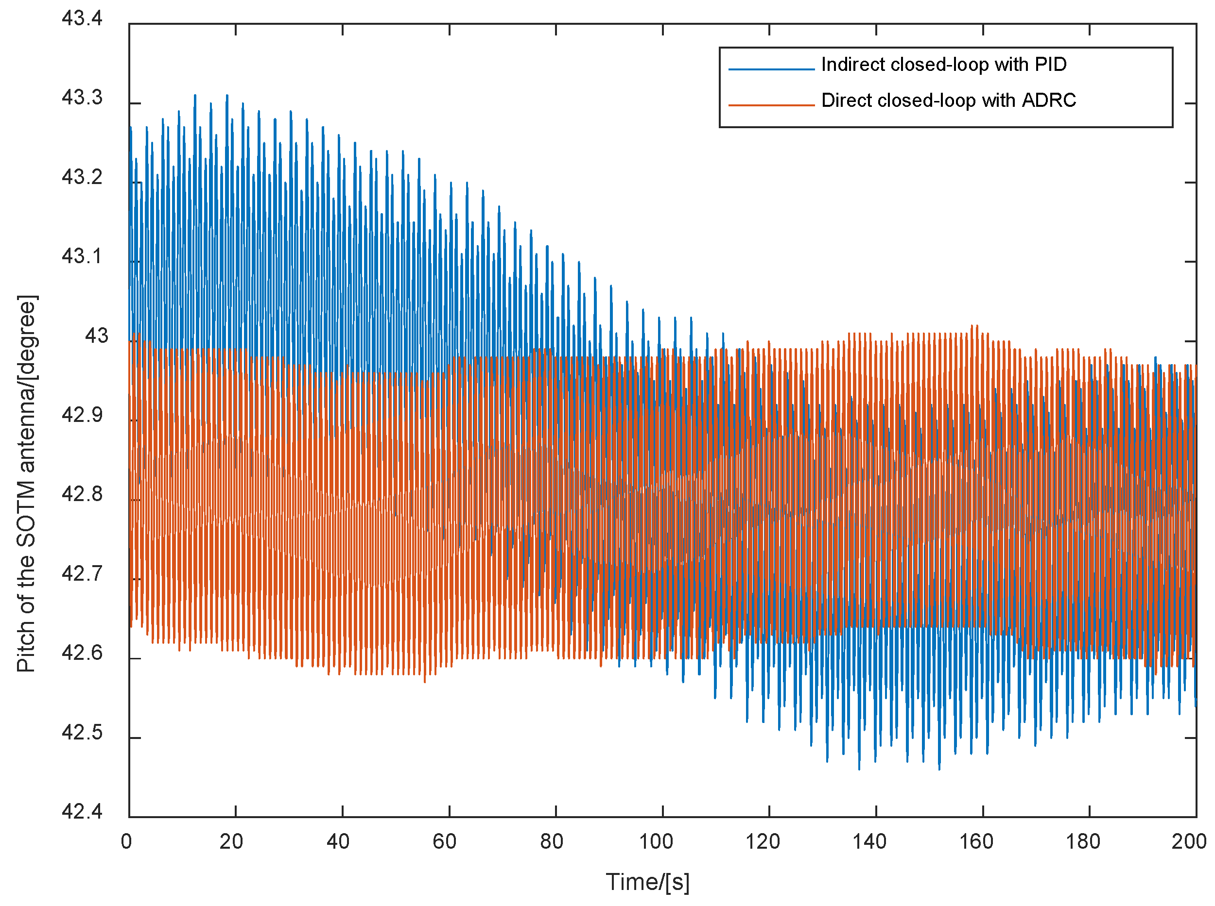
| Azimuth | Pitch | Azimuth | Pitch | |
| Max Value | 141.89 | 43.31 | 141.81 | 43.09 |
| Min Value | 140.72 | 42.46 | 140.88 | 42.53 |
| Mean Value | 141.35 | 42.85 | 141.33 | 42.80 |
| Range | 1.17 | 0.85 | 0.93 | 0.56 |
| Variance | 5.53 × 10⁻² | 2.916 × 10⁻² | 3.58 × 10⁻² | 1.992 × 10⁻² |
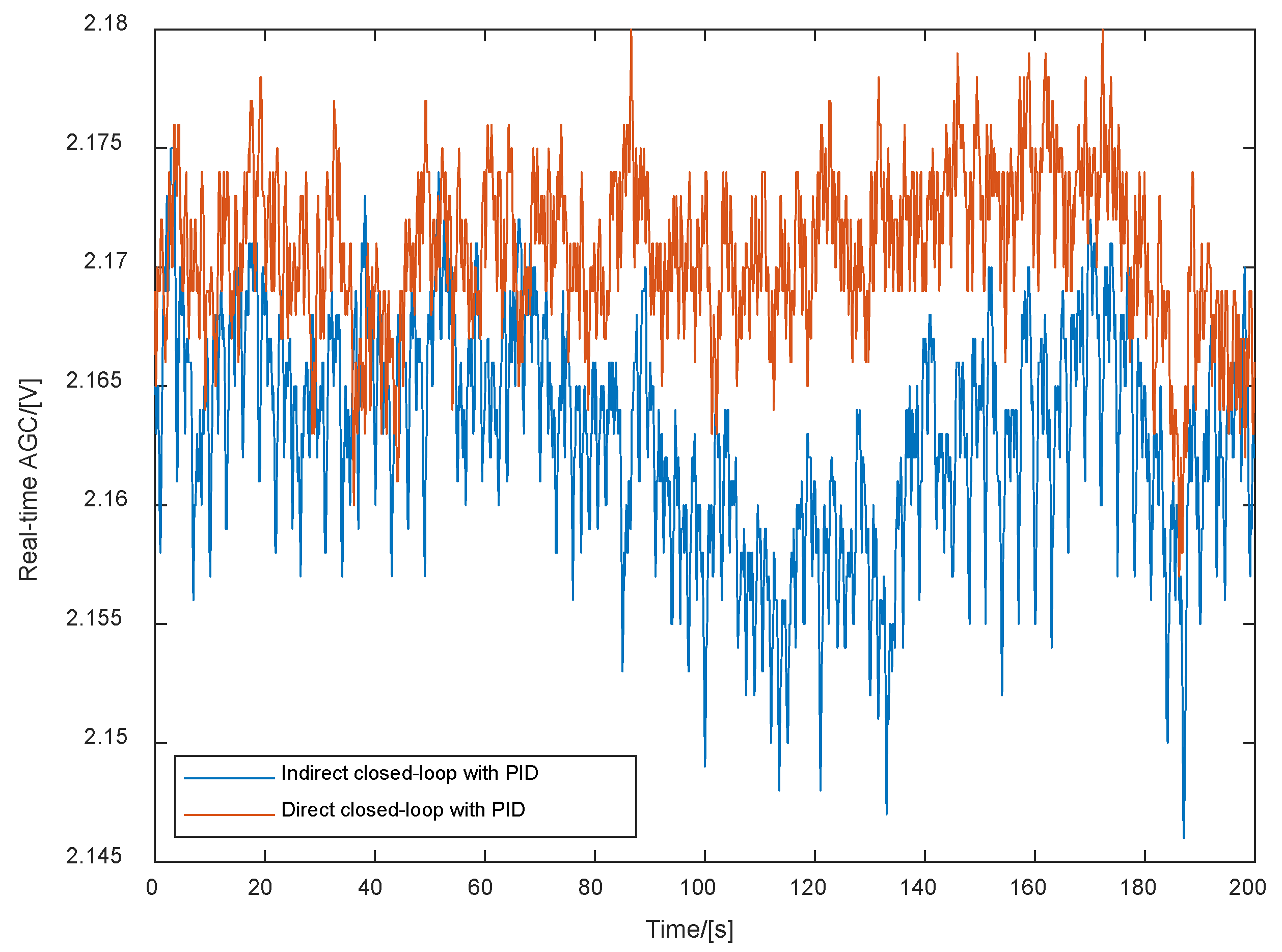
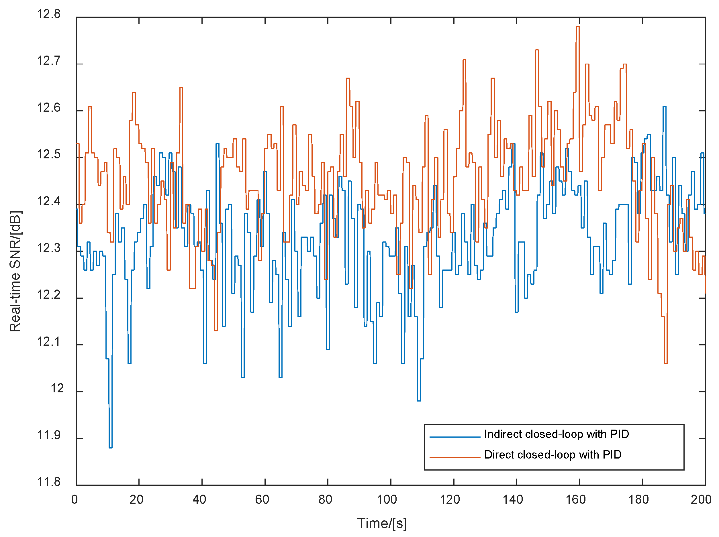
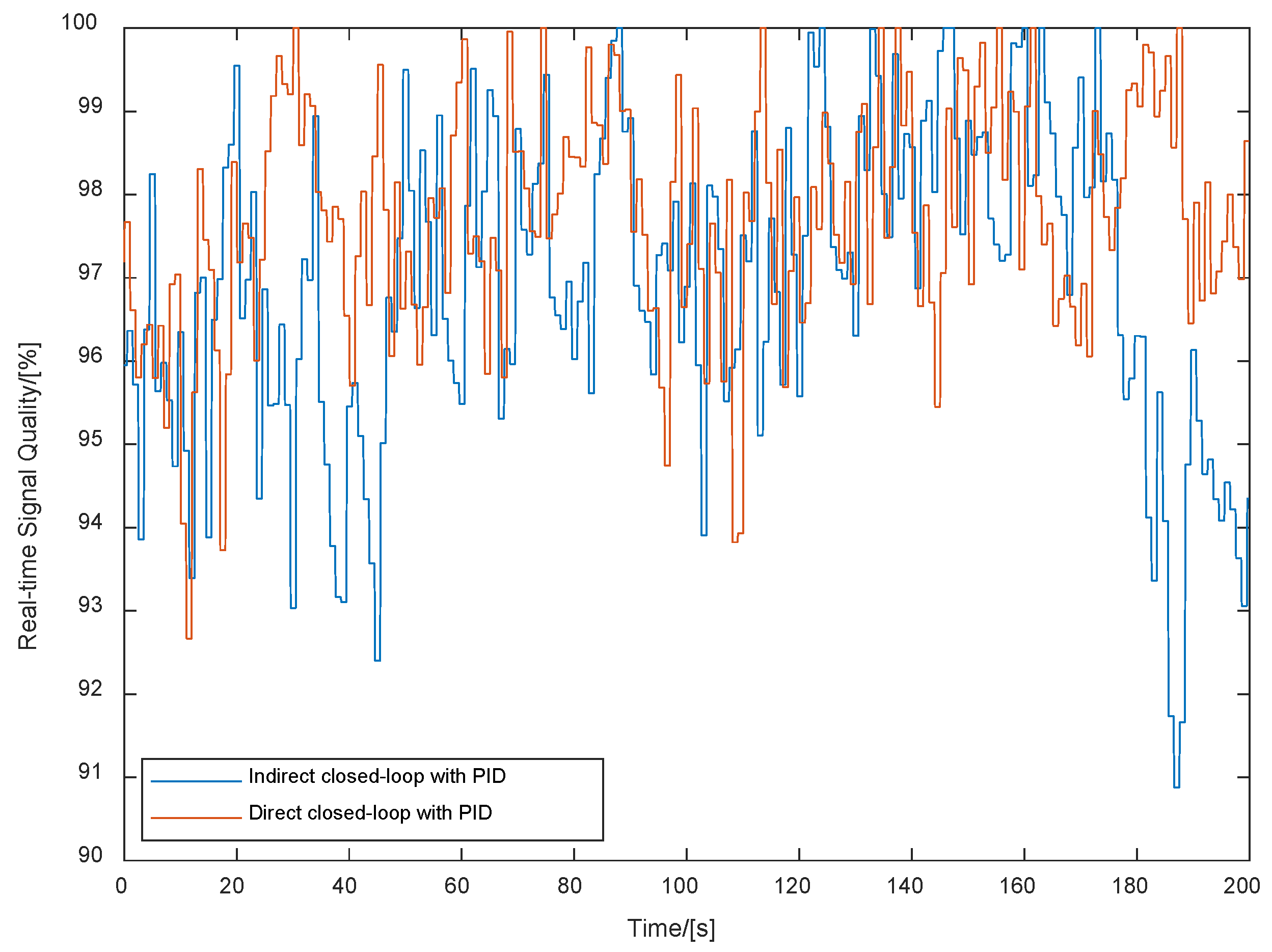
| Indirect Closed-Loop | Direct Closed-Loop | |||||
|---|---|---|---|---|---|---|
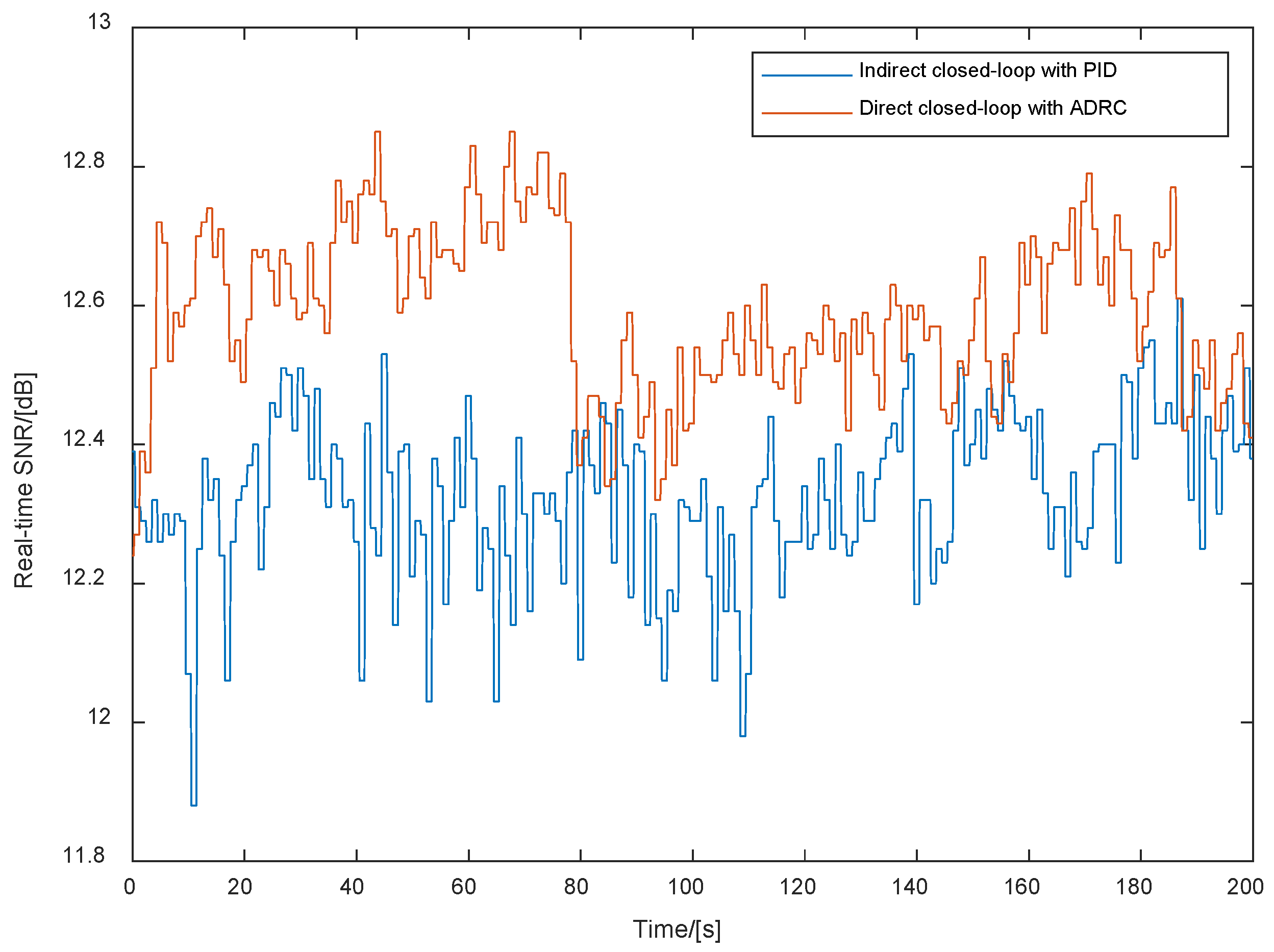
| RTAGCL | RTSNR | RTSQ | RTAGCL | RTSNR | RTSQ | |
| Mean Value | 2.164 | 12.32 | 96.70 | 2.172 | 12.47 | 97.27 |
| Variance | 1.81 × 10⁻⁵ | 1.77 × 10⁻² | 3.85 | 1.45 × 10⁻⁵ | 1.59 × 10⁻² | 2.66 |
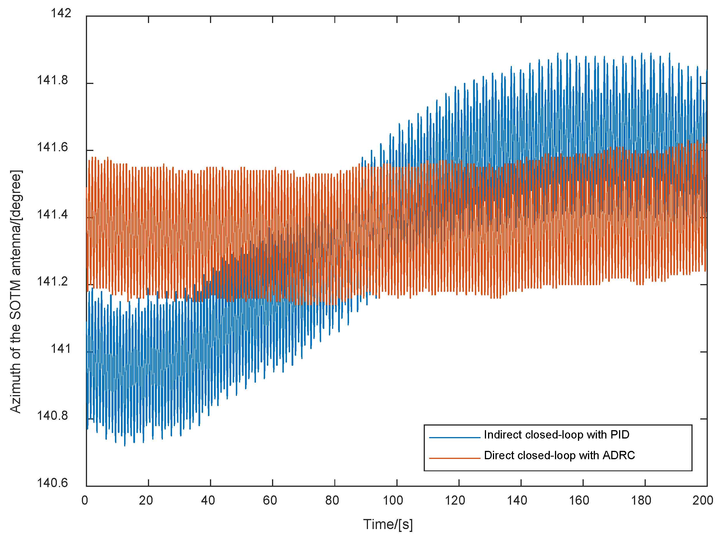
| Azimuth | Pitch | |
|---|---|---|
| Max Value | 141.66 | 43.07 |
| Min Value | 141.02 | 42.55 |
| Mean Value | 141.36 | 42.80 |
| Range | 0.64 | 0.52 |
| Variance | 2.24 × 10⁻² | 1.90 × 10⁻² |
| RTAGCL | RTSNR | RTSQ | |
|---|---|---|---|
| Mean Value | 2.190 | 12.58 | 97.48 |
| Variance | 9.83 × 10⁻⁶ | 1.16 × 10⁻² | 2.21 |
Disclaimer/Publisher’s Note: The statements, opinions and data contained in all publications are solely those of the individual author(s) and contributor(s) and not of MDPI and/or the editor(s). MDPI and/or the editor(s) disclaim responsibility for any injury to people or property resulting from any ideas, methods, instructions or products referred to in the content. |
© 2024 by the authors. Licensee MDPI, Basel, Switzerland. This article is an open access article distributed under the terms and conditions of the Creative Commons Attribution (CC BY) license (https://creativecommons.org/licenses/by/4.0/).
Share and Cite
Ren, J.; Ji, X.; Han, L.; Li, J.; Song, S.; Wu, Y. Direct Closed-Loop Control Structure for the Three-Axis Satcom-on-the-Move Antenna. Aerospace 2024, 11, 659. https://doi.org/10.3390/aerospace11080659
Ren J, Ji X, Han L, Li J, Song S, Wu Y. Direct Closed-Loop Control Structure for the Three-Axis Satcom-on-the-Move Antenna. Aerospace. 2024; 11(8):659. https://doi.org/10.3390/aerospace11080659
Chicago/Turabian StyleRen, Jiao, Xiaoxiang Ji, Lei Han, Jianghong Li, Shubiao Song, and Yafeng Wu. 2024. "Direct Closed-Loop Control Structure for the Three-Axis Satcom-on-the-Move Antenna" Aerospace 11, no. 8: 659. https://doi.org/10.3390/aerospace11080659