Abstract
This paper aims to analyze the stability of a special class of single-channel slow-rotating homing missiles using the Frank–Wall stability criterion. To achieve this, starting from the model of a slow-rolling missile with six degrees of freedom (6 DOFs) in the body frame, a 6-DOFs model in the Resal frame is obtained, which is used to linearize the coupled commanded motion. Based on the linearized model, we obtain the structural scheme of the commanded object and define the flight quality parameters. The obtained linear model has a complex representation (with real and imaginary parts) due to the coupling between longitudinal channels for the rolling missile. Then, the kinematic guidance equations, the seeker equations and the actuator relations using a switching function, specific to the slow-rolling single-channel missile, are defined. The guidance kinematic equations, the seeker equations and the actuator model are linearized in the Resal frame, and the structural diagram of the homing missile is constructed. Starting from this, the characteristic polynomial having complex coefficients is determined and then analyzed with the Frank–Wall stability criterion. Based on the analysis, a stability range is determined for the navigation constant , and a minimum and possibly a maximum limit for the time to hit the target is obtained. The stability range defined for the navigation constant in the linear model is finally validated in the nonlinear model in the body frame.
1. Introduction
In modern weaponry technology, slow-rolling missiles play a significant role in combating close air targets. In anti-aircraft combat, due to the high angular velocity of the target line of site, the missile is directly self-guided, using a proportional navigation method. This method does not ensure a direct hit of the target but achieves a sufficient reach to the proximity fuse so that the warhead destroys the target (because an aircraft does not have armor elements).
If the velocity regime is supersonic, the missiles can use aerodynamic command (canard), effectively performing the target interception maneuver. The advantage of using slow-rotating missiles lies primarily in reducing their size and, implicitly, their mass. At the same time, the rotation cancels the disturbing force and torque due to aerodynamic or gasodynamic asymmetries. Thanks to rolling rotation, the control can be carried out on a single channel, i.e., through a single pair of canards, which reduces the size of the control system and the required energy, leading to a portable missile system known as a man-portable air defense system (MANPADS).
The problem of rotationally guided missiles has been addressed in several stages and forms in the literature. Some of these works refer to two-channel rolling missiles [1,2,3] and others to single-channel missiles with time-modulated command [4,5,6,7]. Among the two-channel rockets, there is a group of papers dealing with double-rotational guided projectiles, in which the projectile body rotates at a very high velocity in order to ensure gyroscopic stability, and the tip of the projectile, which rotates at a lower velocity, has a cruciform canard for trajectory control and improved accuracy [8]. Regarding two-channel rotational missiles, several recent works analyze the design of the autopilot with a double [9] or triple feedback loop [10]. At the same time, other papers aim to assess the stability of precession motion (conical) [1,2,3] or influence of erroneous signal conditions introduced by the target tracking system [9,11]. Another category of papers aims to define sensors with which to determine the attitude, especially the roll angle of the rocket necessary to the command signal [12,13]. The paper [12] presented a new type of combination of a silicon micro-gyroscope; it mainly consists of two perpendicular installations of the micro-mechanical pendulum and the circuit. The combination can demodulate the yaw angular velocity, pitch angular velocity and the spin angular velocity of the rotary missile. The results show that it works very well in the rotating missile attitude control system. The paper [13] proposed the two-step adaptive augmented unscented Kalman filter algorithm to calibrate the biaxial magnetometer, which allows accurate estimates of the missile roll angle.
The paper [14] addressed the optimal problem of the minimum-time attitude control of a spinning missile. A single reaction jet provides the necessary transverse moments. The missile is assumed to have some arbitrary initial transverse angular velocity, and it is desired to take it to some final attitude in a minimum time while reducing the transverse angular velocity to zero.
Since we intend to address the case of the single-channel missile, we will analyze in detail the results obtained in papers [4,5,6,7].
In [4], a digital controller is proposed to replace the classic analogue time-modulation controller. As shown in the paper, replacing the analogue phase control with the digital amplitude control can ensure the decoupling of the yaw from pitch and thereby eliminate the error introduced by the actuator’s delay and the noise from the sensors. The proposed solution’s disadvantage lies in complicating the missile’s control and implicitly increasing its cost.
In [5], the stability of the commanded motion regarding the rocket with single-channel rotation is analyzed based on the linear form of the equations of motion with the development of closed analytical solutions. A feature of the analysis is that it works with the command in the body frame, while the equations of motion are constructed in the Resal frame (which does not participate in the roll rotation). The order to command switch is built based on series development, separately analyzing the ideal case with the rectangular command and the case where the command shape contains a delay.
The paper [7] analyzes the possibility of controlling an autonomous flight rocket with roll rotation and a single channel with reactive command. The classic solution of the Reaction Control System (RCS) with six reactive nozzles which ensure the complete control of the attitude of the rocket, including the roll, is compared with the solution with only two reactive nozzles that provide attitude control in pitch and yaw, leaving the roll angle free, which allows the roll rotation of the rocket.
In paper [6], starting from the equations of motion written in the Resal frame, a linear model of the command motion for the slow-rotating rocket is constructed. Due to the coupling between channels given by gyroscopic and Magnus terms, the linear model is constructed with complex coefficients, highlighting both nutation and precession motion and defining the flight quality parameters. The linear development of the commanded motion ends with constructing a structural scheme of the commanded object specific to the slow-rolling missile with complex coefficients. Unlike work [5], which uses serial development, in work [6], the generation of the switch command for a single-channel missile is conducted considering the sign of a trigonometric expression dependent on the roll angle, as shown in [15]. Further, in the paper [6], two models of slow-rolling single-channel guided missiles are analyzed, the portable anti-aircraft homing missile and the portable anti-tank wire-guided missile. Unlike work [5], which forms the command in the body frame, in work [6], starting from the time-modulated command, an equivalent command is obtained in the Resal frame. Based on this equivalent command, the structural diagrams of the guided missile are built for the two cases: a homing missile and a wire-guided missile. Given that the structural schemes have complex coefficients, the paper was limited to determining in the case of the wire-guided rocket the roots of the characteristic polynomial and the phase–frequency/amplitude–frequency diagrams, highlighting the differences from the case of the non-rolling rocket.
In the present paper, we aim to develop the results obtained in paper [6] by analyzing the stability of the single-channel slow-rolling homing missile using the Frank–Wall stability criterion [16] used in papers [2,3] for the case of a two-channel slow-rolling missile. The essential difference between the two-channel and the single-channel missile consists in the way of forming the command. Thus, if in the two-channel missile we have a proportional deflection with both canards, in the case of the single-channel rocket, we have only one maximum deflection of one of the canards, time modulation, by a switching function. The command orientation is defined by the phase and the amplitude by the filling factor, parameters which will be detailed later. Unlike papers [2,3], which develop a third-order characteristic polynomial, we will also consider the time constant of the target tracking system (seeker), which will lead to a fourth-order characteristic polynomial. This introduces an additional stability condition that will be analyzed in detail. At the same time, the influence of the phase shift introduced by the delay of the actuator and the imprecision of determining the roll angle will be analyzed. In order to facilitate the understanding of this paper, some essential elements introduced in the paper [6] will be resumed. For detail, we recommend reading the original work [6].
In this paper, we will distinguish between slow-rolling missiles (max 30 rot/s) aerodynamically stabilized by a tail and gyroscopically stabilized projectiles with a fast roll rotation (minimum 300 rot/s).
The novelty of this paper consists of the following:
- The analysis of the stability of single-channel homing missiles with slow roll using the Frank–Wall stability criterion. This analysis follows the influence of the main parameters in the missile’s guidance system, and for some of them, restrictions and stability domains will be defined.
- The determination of the Frank–Wall (F-W) stability parameters for fourth-order polynomials; the calculation procedures are detailed in Annex D of this paper.
- The detailed structural scheme of commanded movement for a slow-rolling missile.
- The detailed structural scheme for the homing slow-rolling missile with a single channel.
- The analysis of the stability and command derivative magnitude from the relation (61) and of flight quality parameters from relations (63), (64), (66), (81) and (83).
- The expression of average equivalent canard deflection in nonlinear (147) and linear form (148).
- The validation of linear analysis with the F-W criterion using a nonlinear model (Section 10.4)
2. Equations of the General Motion in the Body Frame
First, we will build a model with six degrees of freedom (6 DOFs) in the body frame.
2.1. Kinematic Equations Using Attitude Angles
The orientation of the body frame related to the local (start) frame is defined according to [17]. We will start by constructing the rotational matrix between the local and body frames to deduce kinematic equations using Euler-type attitude angles. For this purpose, starting in the local frame and ending in the mobile ground frame (), a 180° rotation around the axis is necessary, after which, in order to overlap the mobile ground frame () over the axes of the body frame (), we successively apply three rotations with angular velocities , and around the axes and , respectively:
The rotational matrix from the local frame to the body frame is as follows:
Having defined the direct rotation matrix , one can write the connection between the velocity vector components in the local and the body frames:
Multiplying left by the inverse matrix yields the relation necessary to express the translational velocity components from the body frame, connected to the missile, in the local frame.
where .
To determine the connecting matrix between the derivatives of attitude angles and the components of rotational velocity, we start from the following vector relation:
Moreover, given that the rotation around its axis does not produce any effect, the relation can be written as follows:
hence the following:
Determining the inverse of the matrix, we finally obtain the following:
Developing the relations (2) and (6), the systems of differential equations sought are obtained:
respectively,
2.2. Dynamic Equations of Motion in the Body Frame
The main notations and symbols are consistent with the standards [17,18].
Considering the missile as a body with variable mass and applying the momentum theorem and the angular momentum theorem, the established dynamic equations of motion [19,20] written vectorially are of the following form:
in which the terms due to changes in mass and moments of inertia are contained in the right member of the relations, where we denoted the following: —mass; —velocity; —aerodynamic force; —weight; —thrust; —angular momentum; —aerodynamic torque; and —gasodynamic torque.
By explaining the absolute derivative of velocity and of angular momentum vectors in the body frame, the previous relations become the following:
For the further development of these relations, the forces and torques applied by components according to the axes of the body frame are explained as follows:
where the components of gravitational acceleration are obtained from the following matrix relation:
in which the rotation matrix was previously defined.
In order to bring the equation to the matrix form, the vectors of velocities and angular momentum are also explained by projections according to the axes of the body frame:
The components of angular momentum can be obtained from the following matrix relation:
where represents the matrix of moments of inertia. Developing the vector products of relations (10) and considering the components of the previously explicit terms, one obtains the matrix form of the equations of general motion in the body frame. Thus, the translation equation becomes the following:
where , and is the skew-symmetric matrix associated with the angular velocity vector :
Relations (15) can also be put in the following form:
where we defined the components of the applied forces as ; ; and Similarly, the rotation Equation (10) acquires the matrix form:
For axially symmetrical configurations, the inverse of the matrix of moments of inertia acquires the diagonal shape:
Equation (18) can be put into the following form:
where the components of the applied torques are ; ; and .
3. Equations of the General Motion in the Resal Frame
Unlike classical aircraft, with stabilized roll, in the case of a rolling rocket, most authors [19,20,21], in order to obtain the equations of motion, use a quasi-linked frame (non-spinning body frame), called the “Resal” frame, which has the specificity that it does not participate in its roll motion (Figure 1).
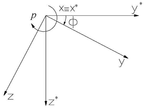
Figure 1.
The Resal frame and body frame connected to the rocket.
The advantages of using this frame are that by isolating the gyroscopic coupling terms, the equations of motion are brought to a form similar to that of the stabilized-roll equations of an aircraft, allowing the use of common study methods, at least in terms of their linear form. Next, we will rewrite the equations of general motion in the body frame, but we will write them this time in the Resal frame. For all the elements in Resal frame we use the symbol “*”. To reformulate the general equations, we start from the observation that the elements of motion in the body frame () are obtained from the quasi-linked frame () using the rotation matrix:
As shown in [6,20], we can express the terms of the dynamic equations from the body frame in the quasi-linked frame. Thus, the velocity components in the body frame become as follows:
and their derivatives are as follows:
Considering that , the components of the rotational velocity in the body frame are expressed as follows:
and after derivation become as follows:
Expressing the force and torque components containing the applied terms (aerodynamics, propulsion and weight) and the skew-symmetric matrix attached to the angular velocity vector in the Resal frame, as shown in [6], multiplying the relations of the dynamic equations in the body frame by the inverse of the rotation matrix, , yields the following:
where
Comparing these equations with the relations (17) and (20) obtained in the body frame, it is observable that in the momentum Equation (27) the gyroscopic coupling term appears between the longitudinal channels. This is due to the rotational motion in roll. From the first line of the matrix relation (27), in order to bring the previous relations to a more suitable form, we can write , with the Euler dynamic equations taking on scalar form as follows:
The kinematic equations, written with elements of the quasi-linked frame (Resal), will coincide with (7) and (8) for the particular case where the roll angle is null. Thus, from the Euler kinematic Equation (8), the following is obtained:
The equation of roll angular velocity becomes a connecting relation between quasi-linked components:
Finally, the other kinematic equations, corresponding to relations (7) expressing the connection between the velocity components in the local frame and the quasi-linked frame, become
4. Basic Movement and Maximum Maneuverability
Determining the basic movement is first necessary to linearize the equations of motion in the Resal frame. For this, we make the hypothesis that the movement is carried out strictly in the vertical plane with constant velocity, at a given height.
4.1. Basic Movement
With the notations from Figure 2, the equilibrium equations in the vertical plane of the Resal frame are written as follows:
where we denoted the lateral acceleration:.
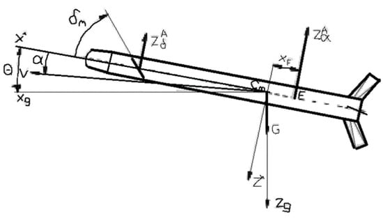
Figure 2.
Basic motion elements in the case of the aerodynamically controlled missile.
In this case, relations (33) becomes
A development of the aerodynamic coefficients containing rotational terms is considered:
where the dimensionless rotational velocity is .
Furthermore, this development is introduced into the system of Equation (34) defining basic motion:
where
As shown in [20], if a rotational velocity and a value of the climb angle (γ) are imposed, and the following is denoted:
where
a system of equations is obtained, and it is solved iteratively for incidence and angular canard deflection:
The diagrams of the equilibrium incidence and canard angular deflection according to the Mach number are presented in Figure A11 and Figure A12 in Appendix B.
4.2. Maximum Maneuverability
If the maximum equivalent deflection angle for single-channel missiles is considered known as follows:
and a value of the climb angle is imposed, the system (36) can be put in the following form:
Considering
where
a system of equations is obtained, which is solved iteratively for incidence and rotational velocity:
From that, we obtain the maximum load factor (Figure A30):
where is called the reduced gravitational acceleration [22].
5. The Linear Form of the Equations of Rapid Motion around the Center of Mass
Using a quasi-linked frame (Resal) for missiles with roll rotation, the equations of rapid motion in the vertical and lateral planes can be grouped and analyzed. For this purpose, it is assumed that the elements of slow motion and roll are “frozen” at their equilibrium values, the perturbation introduced into the system developing only for rapid motion around the center of mass, which, as we will show later, cannot be analyzed separately on each channel, being, in fact, a unique spiral evolution. Also, the higher-order terms from the development of the aerodynamic coefficients, containing small parameter products, will be neglected.
To analyze this motion, we start from the symmetrization of the dynamic equations by the axes of the Resal frame. For this, it is considered that the components of the disturbing force given by aerodynamic and gasodynamic asymmetries are cancelled due to rotation. The remaining perturbations are those due to gravitational acceleration, which generates an asymmetry between the incidence angles and which by gyroscopic terms also affect the lateral plane and those due to wind (disturbance due to wind, from the point of view of the analyzed motion, can induce only additional incidences, the variation in velocity modulus, being specific to slow motion). In addition, due to rolling, the aerodynamic coefficients contain Magnus coupling terms, which appear on both channels. With these specifications, linearizing (17), we obtain the following:
where the velocity components define the incidences according to the axes of the Resal frame:
and the aerodynamic coefficients are
Considering the basic movement, we have the following:
If the incidence in the vertical plane is considered small, the previous relations take on the following approximately symmetrical form:
In this case, Equation (47) can be brought to the following form:
where in the components of the permanent perturbation , both gravitational terms and the remaining terms by the approximation made when symmetrizing the equation of the angle of incidence are found.
Next, we will rewrite the dynamic equations of rotation. We will consider the gyroscopic coupling terms highlighted by the transition from the body frame to the Resal frame and consider null the components of the disturbing moment from aerodynamic and gasodynamic asymmetry. In addition to the conditions imposed on the stabilized-roll base motion, we will consider that the evolution in the vertical plane is translational, i.e., . At the same time, as we did in the case of translation equations, in the pitch moment equation development, the terms corresponding to the slow mode will be considered null. Similarly, the yaw moment equation development will not be affected by the roll motion, which is also considered frozen. Instead, gyroscopic coupling and Magnus terms arising from rotational movement around the longitudinal axis will be highlighted. With these additional clarifications, linearizing (20), we obtain the following:
For coupling the equations, the following dual notations are made:
valid for the case where is small. Actually, these parameters represent the stability and command derivatives that will be presented graphically in Appendix B of this paper.
Next, we define the complex quantities:
where .
The Equations (52) and (53) can be brought to the following form:
Its homogeneous form, after applying the Laplace transform, is as follows:
The characteristic polynomial becomes
Alternatively, after separating complex terms:
The characteristic polynomial contains coefficients with the real part corresponding to the pitch motion and the imaginary part given by coupling with the yaw motion. However, due to the symmetry evidenced by the relations (54), the characteristic polynomial can contain coefficients with the real part corresponding to the yaw motion and the imaginary part corresponding to its coupling with the pitch motion. This observation remains valid for further motion analysis coupled with slow roll. Concluding, for the complex form of motion, the relations obtained describe a single motion with coupling elements from the other.
To analyze this expression and those that will be elaborated on later, evaluating the order of magnitude of the main parameters is useful, allowing us to keep only important terms in approximate relations. For this, in addition to the reference time , also known as the aerodynamic second [23], which is a small parameter, in [22], the following dimensionless parameters are also defined:, called the reduced mass of the aircraft or relative density, and , called the reduced moment of inertia in pitch, where is the radius of inertia of the aircraft for the pitch axis being given by the relation . In this case, the mass and pitch moment of inertia of the missile shall be expressed as follows:
As an order of magnitude, it is observed that the reference time is small, while the reduced mass and reduced moment of inertia in pitch are large.
Next, we will rewrite the main coefficients of the equations of motion previously defined, now including these parameters, obtaining the following:
where we used the dimensionless angular velocity in roll:
With the above notations, after dropping the secondary terms, the characteristic polynomial (59) can be approximated as follows:
where and will be defined in the next section.
In order to evaluate the approximate relations (61), below, we present comparatively the roots of the characteristic polynomial obtained with the exact relation (59) and approximate relation (63).
Based on the next comparative diagrams for the roots of the characteristic polynomial (Figure 3 and Figure 4), as well as the effective values of the stability derivatives indicated in Annex B, the approximation form (61) can be considered valid. In order to obtain a simple structural scheme, we will use the approximative form (61) of the stability derivatives in the linear model, which will not contain all Magnus terms. Later, in the nonlinear model, the complete form of the development of the aerodynamic coefficients will be considered.
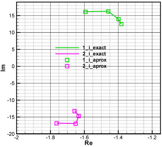
Figure 3.
The roots of the characteristic polynomial in phase 2—initial.
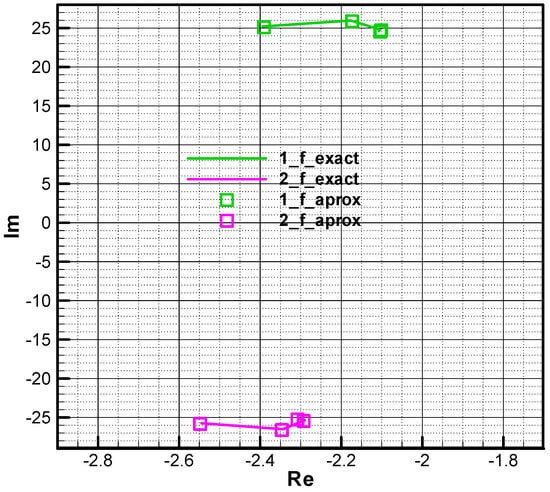
Figure 4.
The roots of the characteristic polynomial in phase 2—final.
6. The Flight Quality Parameters
In the case of aerodynamically stabilized slow-rolling rockets, where the center of pressure is behind the center of mass, the notations are entered as follows:
where represents the angular rate of precession, with dimensionless form , represents static stability (Figure A25), and the characteristic polynomial (63) with the coefficient of the free term having the real part positive can be written in the following form:
where its natural pulsation and damping factor have the same significance as a stabilized-roll missile:
Sometimes, instead of natural pulsation, its inverse is used:
—time constant of nutation movement.
The natural pulsation, damping factor and time constant according to the Mach number are presented in Figure A26, Figure A27 and Figure A28 in Appendix B.
The roots of the characteristic polynomial, so the eigenvalues of the stability matrix, are given by the following:
Alternatively, if it is accepted that , the roots of the characteristic polynomial can be put in the following simplified form:
where .
Note that since the characteristic polynomial has complex coefficients, its roots are not complex conjugate, the additional complex term is given by the angular rate of precession.
To define the command parameter of the rolling missile, we start from the equations of rapid motion (56) written in the following non-homogeneous form:
the inverse matrix is given by
where is the characteristic polynomial with complex coefficients associated with the previously analyzed homogeneous system.
In this case. the main transfer functions are as follows:
system (69) may be put in the following form:
For the construction of a global structural scheme of the commanded missile system, as was conducted in the papers [6,20], from the relations (72), we shall express the angular velocity of the tangent to the trajectory. For this, we start with the following angular relation:
where
Next, we build a relation of the same type as the system (72):
where
Based on the relations (61), we will seek to bring the angular velocity of the tangent to the trajectory transfer function with input in canard angular deflection to an approximate, simplified form.
Thus, we start with the following form:
or rewriting with the following explicit complex terms:
where the characteristic polynomial is given by (65).
Next, the following notations are made:
the angular velocity of the tangent to the trajectory transfer function with the input in canard deflection can be brought to the following form:
Considering approximate relations (61), we obtain the following:
Due to the large value of the parameter , the first two terms can be neglected, resulting in the following:
where is called the command factor, the parameter means, as in the case of the stabilized rolling aircraft, the advance time on command or the aircraft’s time constant, and is a Magnus term.
Dropping the secondary terms for the aerodynamically commanded missile, the parameters defined by the notations (79) become
Finally, we can also evaluate the components of the normal complex acceleration on velocity, which, if we consider the hypothesis of small incidences introduced when symmetrizing longitudinal motion, have the direction of the axes and of the quasi-linked frame, being given by the following approximate relation:
where
Based on the resulting relations, one can construct the structural scheme of the commanded movement for slow-rolling missiles, shown in Figure 5.
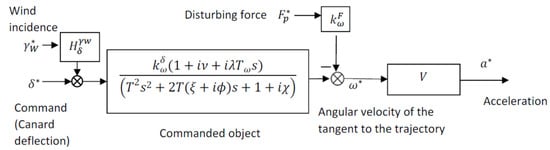
Figure 5.
Structural scheme of commanded movement for slow-rolling missile.
7. The Guided Flight Model
As shown in [20], the guidance kinematic equations will be constructed into a frame linked to the target’s line of sight called the guiding frame (Figure 6). The guiding frame originates at point (, which represents the position of the missile, the axis pointed target , and the axis is in a vertical plane facing downwards and axis horizontally; it follows from the condition of the right frame. The guiding frame is non-inertial.
Figure 6.
Orientation of the guiding frame with respect to the local frame [24].
The angles defining the orientation of the guiding frame with respect to the local frame are given by the following relations:
where and are the coordinates of the rocket in the local frame, respectively, , and , the target coordinates in the local frame.
With the help of these two angles, the rotational matrix is formed, which makes the transition from the local frame to the guiding frame as follows:
Next, we will obtain the guidance kinematic equations in the guiding frame, which is non-inertial.
7.1. Kinematic Guidance Equations
Figure 7 and Figure 8 show the decompositions of velocity and acceleration of the missile and target according to the axes of the guiding frame. Given the general relations of derivation, in a non-inertial frame, one can write the following:
where the relative velocities and accelerations are expressed in the following guiding frame:
i.e., matrices resulting from the following vector products:
in which
Due to rotational matrix (87), we can obtain the velocity and acceleration components (89) in the guiding frame from the inertial frame (local frame).

Figure 7.
Decomposition of velocities in the guiding frame.
Figure 7.
Decomposition of velocities in the guiding frame.


Figure 8.
Decomposition of accelerations in the guiding frame.
Figure 8.
Decomposition of accelerations in the guiding frame.

Knowing these quantities in the guiding frame, next, we propose to obtain the equations of the components of angular velocity and angular acceleration of the guiding frame, equations known as kinematic guidance equations.
Based on the relations (88), the components of relative velocity and relative acceleration in the guiding frame are
respectively,
relations from which the components of angular velocity and angular acceleration of the guiding frame can be expressed; relations which represent the kinematic equations of guidance:
respectively,
Based on the components of velocity of the missile and target in the guiding frame, according to [24], we define the aspect angles of the missile and of the target in the first guiding plane (Figure 9):
respectively, in the second guiding plane (Figure 10):
Also, we have a connection between the angles in first guiding plane (Figure 9):
respectively, in the second guiding plane (Figure 10):
where , are absolute angles of the line of sight, are the missile climb angle and flight path azimuth angle and are the target climb angle and flight path azimuth angle, according to [24]. Based on the components of velocity of the missile and target in the guiding frame, we define the projections of velocity for the missile and target in the first guiding plane:
respectively, in the second guiding plane:

Figure 9.
The first guiding plane [24].
Figure 9.
The first guiding plane [24].


Figure 10.
The second guiding plane [24].
Figure 10.
The second guiding plane [24].

7.2. Linear Form of Kinematic Guidance Equations
The basic motion in proportional navigation is a parallel approach, which is characterized by the fact that the absolute angular velocity of the line of sight and the derivative of the angular velocity of the line of sight are null:
Because in the basic movement the guidance parameters are null (), the guidance components for basic movement shall also be null:
Also, we will consider a stationary basic movement in which the missile and the target evolve with constant velocity in the module.
Based on relations (96), (97), (100) and (101), the Equation (94) become as follows:
Linearizing, we obtain the following:
Considering the angular connection in (98) and (99), the following results from (105):
or yet
Synthetizing, to linearize the angular velocity equations of the line of sight, one can start from the relation (94), obtaining the following:
Denoting the input due to launch error as follows:
we obtain
If the complex components are introduced as follows:
the equation of the absolute angle of the line of sight in complex form is obtained:
Regarding the Equation (95), neglecting the product of small parameters and they become the
following:
Linearizing, we obtain the following:
Considering the angular connection (98) and (99), we obtain the following:
Due to stationary basic movement in which the mobile and the target evolve with constant velocity in the module, the terms and and accelerations can be neglected.
Denoting the input function due to target maneuvers as follows:
we finally obtain
If we define complex components as follows:
the equation of the angular velocity of the line of sight in complex form is obtained as follows:
Considering the coefficients of the guidance equation frozen at the values corresponding to the base motion and the current missile–target distance (R) changing slowly with respect to the guidance parameters, the Laplace transform can be applied to Equation (119), obtaining the following:
where the input function is
Considering that distance is constant and equal to the value at a given moment, the transfer function of the kinematic block becomes
where is considered a frozen parameter corresponding to the distance to the target, and with , we denoted the collision velocity.
7.3. Target Tracker Equations
The equation of the target tracker (seeker) that provides guidance commands in two planes is as follows:
where the control parameters are angular velocities , in the guiding frame defined by the line of sight.
If we linearize, considering that in basic movement the guidance signal is null, we obtain the following:
Defining the complex component of the guidance command as follows:
the equation of the target tracking device in complex form is obtained as follows:
where is the seeker gain, and is the seeker time constant.
After the application of the Laplace transformation, the transfer function of the target tracker (seeker) can be obtained as follows:
a function that will be used for the guided missile system diagram.
7.4. The Command for Slow-Rolling Single-Channel Missile
In [6], two guided missile models were built, one for the homing missile and the other for the wire-guided missile, for which no detailed analysis was made. In Section 3, the equations of motion in the Resal frame are presented. The rapid motion around the center of mass was analyzed by linearizing these relations, and the quality flight parameters of the commanded longitudinal motion, specific to the slow-rolling missile, were defined. In Section 7.2, we built the linear form of the guided kinematic equations and in 7.3 the seeker equations. In order to build a guided flight model for the homing missile, we need the relations that describe the way of obtaining the command—the functionality of the actuator. For this, we start from the expression of the two-channel command, which, considering only the guiding terms, has the following form:
Since in the basic uncoupled guidance equation we assume that the head angle of the rocket coincides with that of the guiding frame , and neglect the angle of incidence in the vertical plane, in order to be able to achieve the symmetrization of the two guiding planes, the command can be put in the following form:
where the following notation was made:
where is the direct rotation matrix with the roll angle.
Next, we will seek to bring matrix expressions to complex form using a polar coordinate system that highlights the module and phase of the guidance command. Thus, if the commands are put in the following complex form:
the relation (129) becomes
On the other hand, as seen in Figure 11, the guidance command can be expressed in polar coordinates as follows:
where
is the command module, and is the command phase.

Figure 11.
Expression of the guidance command in polar coordinates.
Figure 11.
Expression of the guidance command in polar coordinates.

In this case, the command for the two channels (pitch and yaw) in the body frame becomes
where is the phase shift error:
In this relation, we introduce —the command advance angle that is intended to cancel out the delay effect; —the command delay time; and —the roll angle error.
The phase shift value thus introduced, may be due both to the choice of a constant value for the delay compensation angle (which in the case of rotational velocity variation during the trajectory leads to an erroneous phase) and to the poor assessment of the roll angle (required to form the command, with deviation ). Since this phase shift is due to rolling angular velocity, being specific to rolling missiles, we shall eliminate it in the case of the stabilized-roll missile analysis.
To obtain the time modulation of the command for the single-channel missile, it is necessary to use a switching function of the form [15]:
where , called the fill factor, is given by the following relation:
in which is the command module, is the maximum guidance command, and the argument , called the relative roll angle, is given by the following:
where represents the command phase (Figure 11), is the roll angle (Figure 1), and is the phase shift error.
The switching function (136) is applied instantaneously through a nonlinear element, relay-type, with the following pitch canard deflection angle:
To check how the function generates a canard angular deflection correlated with roll rotation, it is necessary to determine the zeros of this function that coincide with the deflection switching points. For this, the expression (136) is put in the form of an equation:
the solutions of which are obtained by imposing, in turn, the following conditions:
For the interval in which obtains values, we have a group of switch points due to the condition , which are .
From the condition , the second group of switch points are obtained. For extreme values of the fill factor , we obtain , which is the maximum command after a certain direction, and for , results in , , which means the null command.
For a better understanding, in papers [6,20], the equivalent deflection was determined for the particular case when the control phase is φ (Figure 11), with a null phase shift error = 0, which drives a positive pitch command.
Next, we obtain the expression of the single-channel command for an equivalent canard deflection in the Resal frame that will be used to define the linear form of the actuator necessary to build the structural scheme of the guided system. For this, we start from the shape of the canard deflection in one rotation period given by the relation (139).
For the single-channel case, considering only pitch deflection , we have the following:
where is the equivalent instant deflection in the Resal frame.
The relation can be reversed:
In this case, the average equivalent canard deflection over one rotation in the Resal frame shall be given by the following:
Considering the command parity for a full rotation, the average equivalent canard deflection becomes
The integral in this relation can be calculated with the diagram from Figure 12, obtaining the following successively:
Thus, having the integral determined from the relation (145) and the relation defining the fill factor (137), the average equivalent canard deflection becomes
and the linear form of the actuator is obtained:
where
is the actuator gain.

Figure 12.
The shape of the canard deflection for one period of missile roll.
Figure 12.
The shape of the canard deflection for one period of missile roll.

Observation
Given that the average equivalent deflection is carried out in a full period of rotation, it can be considered that it follows the command signal in steps, the duration of a stage corresponding to the rocket’s rotation period. If the rocket’s rotation frequency is high enough (over 10 Hz), the output of the actuator may be considered smooth enough to be approximated as continuous.
If the actuator (148) is also added to the transfer function of the kinematic block (122), the transfer function of the target tracker (127) and the commanded object (Figure 5), the structural scheme for the homing missile with a single channel and slow roll rotation can be obtained (Figure 13).
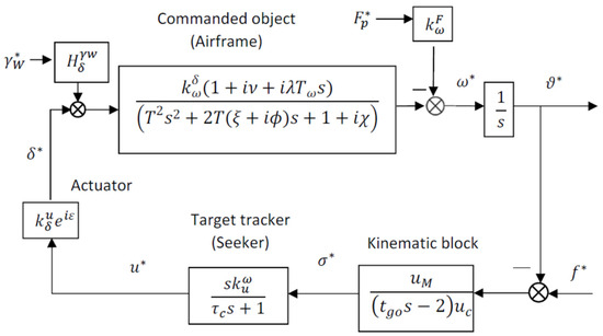
Figure 13.
The structural scheme for the homing missile with single-channel and slow roll rotation.
8. The Guided Flight Stability in the Linear Model
8.1. Determination of Stability Parameters
For system stability analysis, the transfer function of the open system is required:
where we highlighted the modified navigation constant [25], which we will now call the navigation constant:
In this case, the transfer function of the closed system becomes
To check the stability, we develop the characteristic polynomial from the denominator of the transfer function:
Next, we will proceed similarly with [3], based on the work [16], which indicates a method for establishing the condition that the roots of the characteristic polynomial have the real side negative, which ensures the stability of the system. The method is similar to the Routh–Hurwitz stability criterion and consists of checking the sign of a number of parameters equal to the degree of the characteristic polynomial.
Thus, the characteristic polynomial is put in the following form:
where
Stability conditions for systems with characteristic polynomials with complex coefficients are formulated by two theorems in the paper [16]. The first theorem shows that for the nth-order polynomial with complex coefficients to have all the roots with negative real parts, it is necessary and sufficient that the parameters be positive and that be pure imaginary numbers or null. The second theorem shows that the nth-order polynomial with complex coefficients has as many roots with the positive real part as the number of negative parameters.
In the same work, an algorithm for obtaining the parameters , is indicated; the algorithm is presented in Annex D of the paper. These conditions will be referred to as Frank–Wall (F-W) stability conditions in the following after the authors’ names.
Given the 4th-order polynomial from (154), the following is denoted:
The F-W stability parameters are
respectively,
In the previous relations, are pure imaginary numbers in all cases, which, depending on the values and can be null. The only conditions to be verified or imposed are , which, based on relations (157), translates into the following four conditions:
8.2. Non-Rotational Case Analysis
For the case of a non-rotational rocket, in which the phase shift is considered null (), conditions (159) become
which are relations that coincide with the Routh–Hurwitz (R-H) conditions for polynomials with real coefficients.
Next, we are looking for analytical solutions for stability conditions in the case of non-rolling missiles and numerical solutions in the case of rolling missiles.
The first condition (160) provides the lower bound for the remaining interception time (, i.e., the minimum distance to which the missile can approach the target:
The second condition, since it does not contain the navigation constant, may introduce an additional restriction on the remaining interception duration (:
To impose the condition, we construct a quadratic polynomial in and look for its roots:
we make the following notations:
from which the following roots are derived:
with the following discriminant:
If we develop the first root, we obtain an approximate solution:
relation that represents the first condition R-H (161).
It follows that the value of interest is given by the second solution of the Equation (163):
a relation which can be interpreted as a decrease in the stable guided time until , which means an increase in the minimum distance the missile can approach the target.
On the other hand, given the form of the polynomial (163), with the second derivative positive (the coefficient of the quadratic term is positive), if , then the roots are complex, so the second condition is fulfilled all the time. The sign of discriminant depends on the value of the seeker time constant , and if we increase its value, becomes negative.
The third R-H condition limits the upper navigation constant :
Finally, the fourth R-H condition sets the lower bound of the navigation constant :
The first condition, the limitation of the duration of interception, since it does not depend on complex terms, also applies to the rolling missile. For the other conditions, in the case of the rolling missile, we will conduct a numerical analysis based on a calculation model that we present below.
9. Calculus Model
In order to obtain numerical results, we will further specify the data of the calculus model.
9.1. Aerodynamic Characteristics
The aerodynamic characteristics were determined using the configuration in Figure 14, which is typical for the class of missiles analyzed.

Figure 14.
Slow-rolling single-channel homing missile.
In current flight dynamics applications or in the analysis and synthesis of guided systems, it is necessary to know the values of aerodynamic coefficients for certain given situations characterized by Mach numbers, incidences, rotational velocities, canard deflections or flight altitude.
For this purpose, functions are sought to approximate the aerodynamic coefficients in relation to the system’s state variables, functions that, for simplicity, can be chosen by the polynomial form [26,27]. The state variables considered will be small (incidences, angular deflections, rotational velocity), and to highlight the advantages of configuration symmetry, polynomial development will be conducted around zero. Obviously, the coefficients of polynomial development terms remain dependent on the Mach number and possibly the Reynolds number or height.
In the following, considering the specifics of the configuration and the wide range of flight regimes, starting from the aerodynamic coefficients indicated in [26], we introduce additional terms in the development. These terms shall contain rotational and non-stationary motion and combinations with incidences and angular canard deflection.
Using the reference time , rotational velocities and non-stationary translational variables can be considered dimensionless, the notations being according to the following standard [18]:
In addition to these, this paper also uses the dimensionless height defined by the following relation:
Thus, the development of aerodynamic coefficients in the body frame for the slow-rolling single-channel airframe in Figure 14 is given by the following:
The main terms of development of aerodynamic coefficients are presented graphically against the Mach number in Appendix A.
9.2. Mechanical and Reference Characteristics
The mechanical characteristics of the model are indicated in Table 1.

Table 1.
Mechanical characteristics.
For the considered configuration, the reference length is , the reference surface is , and the maximum angular canard deflection is .
9.3. Thrust Characteristic
The thrust characteristic of the model is shown in Figure 15.
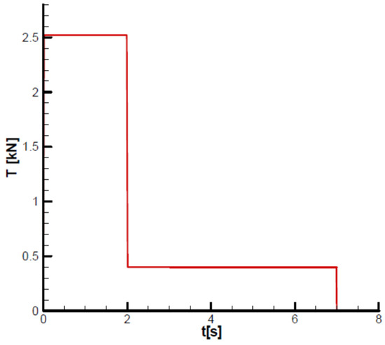
Figure 15.
Thrust diagram.
Given the thrust diagram and the table of mechanical characteristics, the missile will have two flight phases: a first phase of acceleration (boosting) and a second phase of marching flight, with approximately constant velocity, as shown in the velocity diagram from Section 10.4.
9.4. Time Constants and Controller Gains
As basic data for the linear model, the following parameters were considered:
- Constant navigation indicated as the optimal value for the PN method [28];
- The time constant for the target tracker ;
- Time to reach the target starting from the second phase of flight ;
- Rolling rotational velocity close to that indicated in Section 10.4 ;
- Calculation altitude ;
- Phase shift .
10. Stability Analysis of the Single-Channel Homing Slow-Rolling Missile
10.1. Organization of Results
Appendix B presents the incidence and equilibrium deflection angle of the canard and the main flight quality parameters for the initial and final moment of the second phase of flight (marching mode) according to the mechanical data from Table 1. Given the velocity diagram from Section 10.4, the field of analysis and the height were chosen, corresponding to the field of altitude to this phase of flight.
Based on the relations (155) and the flight quality parameters from Appendix B, the characteristic polynomial coefficients were determined. They are also calculated at the beginning and end of the second phase with respect to the Mach number and altitude. The characteristic polynomial coefficients, both real and imaginary, are shown graphically in Appendix C. Based on the relations (157) and the characteristic polynomial coefficients, the Frank–Wall coefficients ( were determined and are graphically shown in Appendix C. For the basic input data considered, stability criterion F-W is met: , as we can see from Figure A39–Figure A42.
10.2. The Root Locus
Next, we will analyze the root locus of the characteristic polynomial.
To begin, we shall consider the basic test case set out in Section 9.4 for the second phase of flight at two points, at the beginning (Figure 16) and the end of the phase (Figure 17). The analysis is conducted on the range of Mach numbers corresponding to phase 2 () and height . A first observation of a general nature is that the roots do not have a symmetrical distribution with respect to the real axis, as in the case of stabilized-roll rockets, where the characteristic polynomial has real coefficients. There are four roots of the polynomial, as follows:
- -
- -
- Root 3 is large in the module, with a negative real part and a small complex part, due to the target tracker response time.
- -
- Root 4 is small in the module, with a negative real part, with a small complex part due to the guidance loop.

Figure 16.
The roots of the characteristic polynomial in phase 2—initial .
Figure 16.
The roots of the characteristic polynomial in phase 2—initial .


Figure 17.
The roots of the characteristic polynomial in phase 2—final .
Figure 17.
The roots of the characteristic polynomial in phase 2—final .

In Figure 18 and Figure 19, the position of the four roots is shown when an increased navigation constant is used. There is a shift to the left of root 4, while roots 1 and 2 move to the right and may have real positive values initially but negative values in the end. It will be shown that the chosen value for the navigation constant, in this case, is greater than the permissible limit resulting from the third condition of F-W for the initial moment.
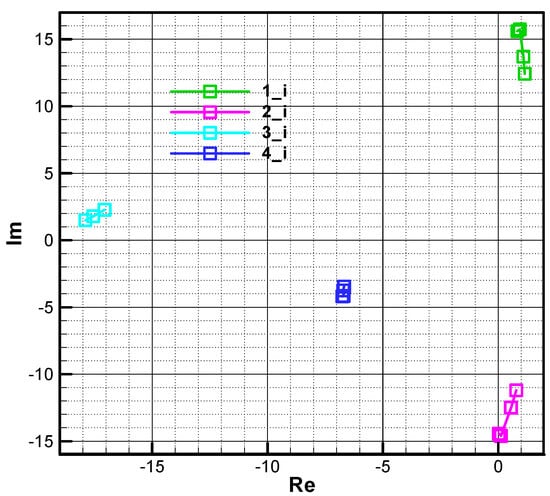
Figure 18.
The roots of the characteristic polynomial in phase 2—initial (.
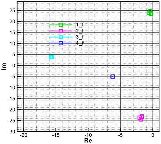
Figure 19.
The roots of the characteristic polynomial in phase 2—final (.
Figure 20 and Figure 21 show the influence of increasing the time constant of the target tracker. Thus, if the time constant value is doubled (, displacement to the right of the third root is obtained without significantly affecting the other roots.
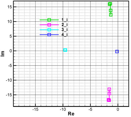
Figure 20.
The roots of the characteristic polynomial in phase 2—initial .
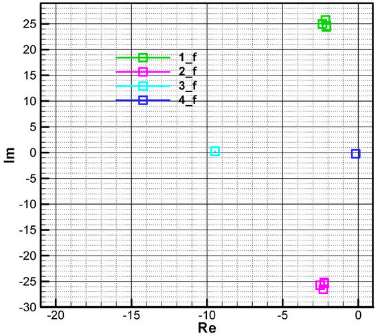
Figure 21.
The roots of the characteristic polynomial in phase 2—final .
In Figure 22 and Figure 23, the influence of phase shift on the root location of the characteristic polynomial is analyzed. Thus, if the phase shift is cancelled , a symmetrization of roots 3 and 4, which are on the real axis (the imaginary part is null), is obtained, while roots 1 and 2 remain asymmetrical with respect to the real axis due to precession, as follows from the relation (67).
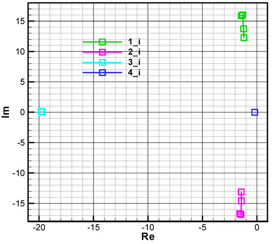
Figure 22.
The roots of the characteristic polynomial in phase 2—initial .
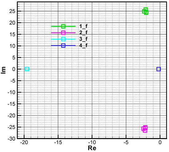
Figure 23.
The roots of the characteristic polynomial in phase 2—final .
In Figure 24 and Figure 25, the influence of the parameter on the location of the roots of the characteristic polynomial is analyzed. Thus, if this parameter is subtracted from to at both calculation points (initial and final), a small displacement to the left of the fourth root and to the right of the other roots is obtained. Note that initially, root 1 may have the real part positive (Figure 24), which leads to instability, but finally it cancels out, with root 1 having the negative real side (Figure 25).
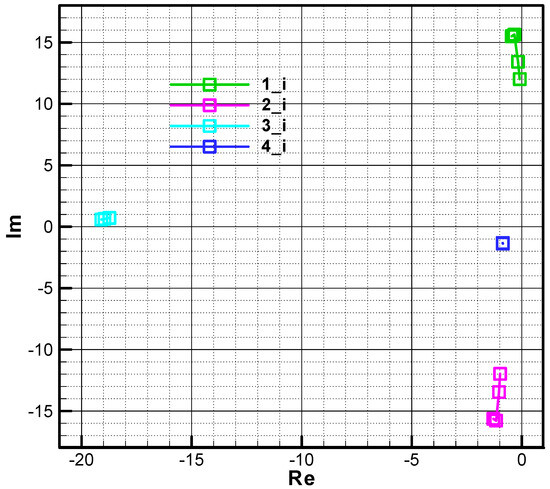
Figure 24.
The roots of the characteristic polynomial in phase 2—initial .
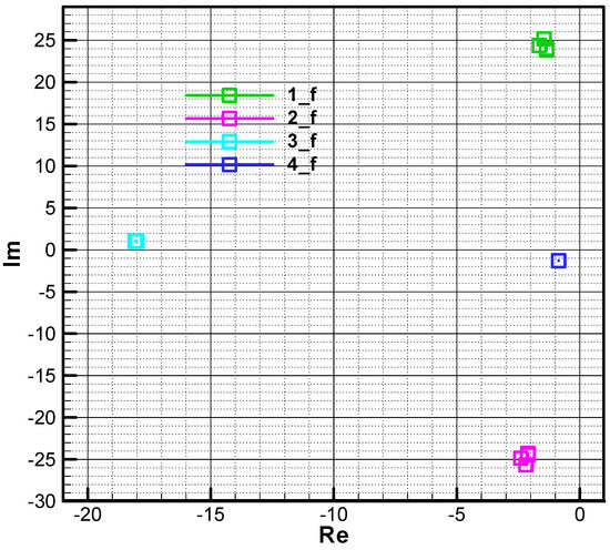
Figure 25.
The roots of the characteristic polynomial in phase 2—final .
10.3. Constraints Due to Stability Conditions
Next, we will analyze the constraints on the target’s time to hit () and the navigation constant () due to the stability conditions of F-W.
10.3.1. Time to Hit the Target
The first stability condition of F-W is identical to the first R-H condition for the non-rolling rocket and refers to the lower limit . It is found that the limit at the final moment is lower than that at the initial moment and increases with velocity (Figure 26).
Figure 26.
The lower limit from the first condition of F-W,
Since the lower limit depends on , we must evaluate its influence. So, if we double the value we obtain the results from Figure 27 for the lower limit . It is observed that doubling the time constant leads to approximately doubling the lower limit of .
Figure 27.
The lower limit from the first condition of F-W, .
As for the second condition of F-W, similar to the R-H case analyzed for the non-rotating rocket, an upper limit for is obtained, which fortunately disappears at the end of the phase, as can be seen from Figure 28.
Figure 28.
The upper limit from the second condition of F-W, .
If we double the time constant , the upper limit of disappears completely, as can be seen from Figure 29.
Figure 29.
The upper limit from the second condition of F-W, .
Synthesizing, increasing the time constant of the target tacker leads to an increase in the lower limit , which is bad because it increases the distance to which the missile can approach the target. However, it can also have a beneficial role by eliminating the upper limit of .
10.3.2. Navigation Constant
The third stability condition of F-W gives the upper limit of the navigation constant indicated in Figure 30. It is higher at the flight phase’s end and slightly decreases with velocity. For comparison, they are presented in the same diagram for cases without rolling, marked with ak2h_i, ak2h_f, and rolling cases, marked with ak2_i, ak2_f. It can be noted that at the beginning of the flight phase, the values with rolling are very close to those without rolling, while at the end of the phase, the values without rolling are higher than those with rolling.

Figure 30.
The upper limit of the navigation constant (.
For the fourth stability condition of F-W, in the case of a rolling rocket, the minimum value of the navigation constant is also obtained (Figure 31). It can be seen from the diagram that in the case of rolling, the minimum value is slightly higher than in the case without rolling, in which case the minimum value is . It is also noted that, for the field of interest, the final value is lower than the initial one, and both increase with the velocity (Mach number).
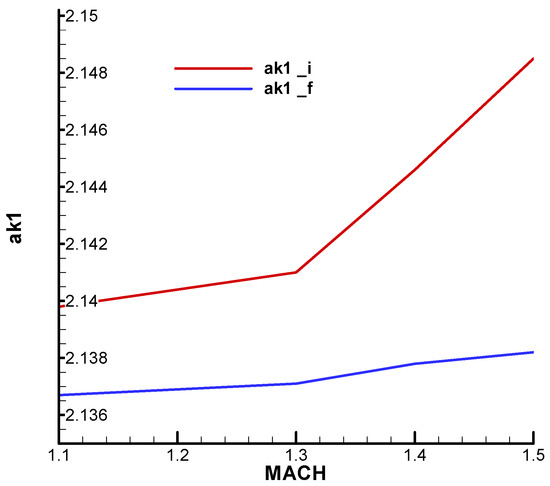
Figure 31.
Lower limit of the navigation constant .
Summarizing the last two cases, it is found that in the rolling case, the range of the navigation constant decreases both in terms of the lower limit, which is slightly higher (Figure 31), and in terms of the upper limit, which is significantly lower (Figure 30).
Note that this difference in the upper limit is mainly due to phase shifting ; in its absence, the limits with rolling are almost identical to those without rolling, as can be seen in Figure 32.

Figure 32.
The upper limit of the navigation constant without phase shift (
10.4. Stability Analysis Based on the Nonlinear Model
Based on the dynamic equations of motion in the body frame (17) and (20), kinematic Equations (7) and (8) and kinematic guidance Equation (94), as well as the target tracker Equation (123), switching function (136) with the relative roll angle definition relation (138) and expression of pitch canard deflection angle (139), the nonlinear model of the guided flight of the single-channel, slow-rolling, homing missile is obtained.
The objective of the nonlinear model analysis is to verify the limits of the navigation constant ( set out in the previous point, such as the lower limit of the parameter . We will consider parameters similar to linear analysis: ; and a tactical situation with a fixed target placed at a distance of 2.5 km and a height of 2.5 km. The choice of a fixed target was made in order to simplify the construction of the navigation gain, in which case , and the navigation constant coincides with the modified navigation constant:
From the relation (174), only the first factor can be imposed because it is related to the constructive solution of the target tracker, possibly by an additional amplification constant. At the same time, the second factor is constant , and the third factor depends on the dynamics of the missile, being difficult to control. In this case, we will choose so that, when multiplied by the other two gains, a value close to the desired is obtained. Given the objectives of this section of this paper, we will seek to obtain three navigation gains, the first less than 2.0, representing the defined lower limit of condition 4 F-W; the second close to 3.0, a value used in linear analysis; and the third larger than the upper limit resulting from condition 3 F-W. As previously stated, these values will be determined as a function of time simultaneously with the integration of nonlinear equations of motion that will be conducted in the body frame. Obviously, due to the variation in the third factor , the navigation gain will vary over time, as can be seen in Figure 33. The analysis is performed considering three identical missiles but with different navigation gains, the first below the lower limit, the second within the limits defined in the linear analysis, and the third above the upper limit.
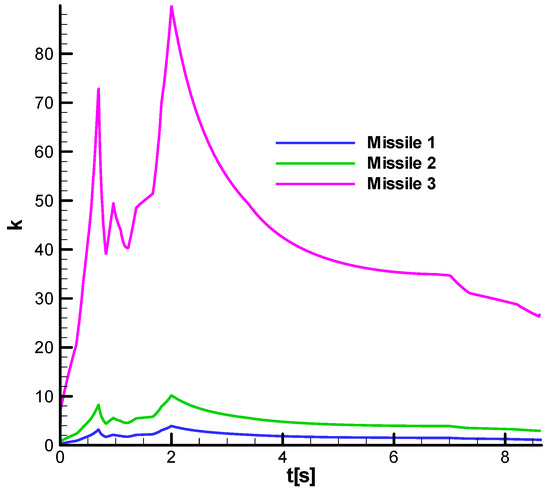
Figure 33.
Navigation gain.
For the three rocket models defined above, Figure 34 shows the velocity diagram that was previously used to define the analysis range in the linear model , which corresponds to the second phase of flight. There are no major differences between the three cases analyzed.
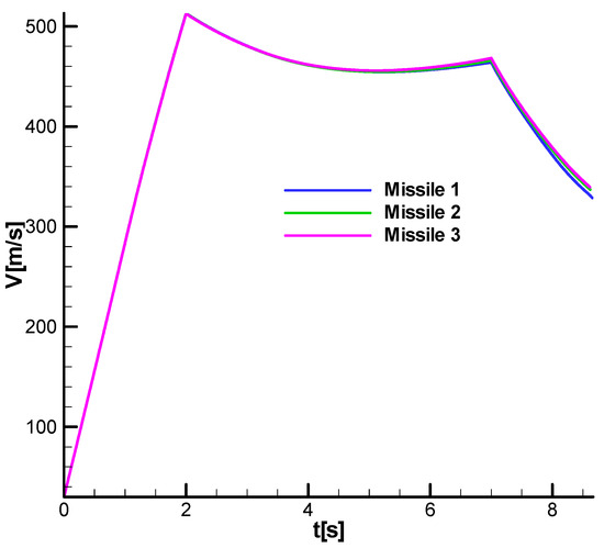
Figure 34.
Velocity diagram.
Figure 35 shows the angular roll velocity diagram based on which the rotational velocity of , corresponding to the second phase of flight used in linear analysis, was chosen. It is observed that the roll velocity follows the velocity profile and does not differ substantially between the three cases.
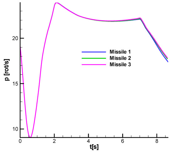
Figure 35.
Roll velocity diagram.
Figure 36 and Figure 37 show the vertical and horizontal projection of the trajectories for the three analyzed cases. From the horizontal projection (Figure 37), it can be seen that all trajectories have a slight deviation to the left of the shooting plane, a phenomenon specific to aerodynamically stabilized slow-rolling rockets. Note that for case 1, with the navigation gain below the limit, the trajectory is more curved than the trajectory in case 2, which is considered a reference case. In contrast, for case 3, with the navigation gain above the maximum limit, the trajectory is less curved than for case 2. From the horizontal projection, we can see that, for case 1, the trajectory of the missile does not reach the target.
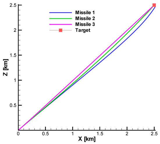
Figure 36.
Target interception—vertical view.

Figure 37.
Target interception—horizontal view.
Figure 38 and Figure 39 show the command fill factor and the command phase. Figure 38 shows that for case 1 with a low navigation gain, the fill factor saturates before reaching the target, which leads to the missile’s inability to continue the guidance process to the target. On the other hand, in case 3, with a large navigation gain, oscillations in the fill factor in the final phase occur, which, in the end, will also lead to the loss of the target. In contrast, in case 2, the reference case, the fill factor increases progressively, reaching a unit value at the moment of reaching the target.

Figure 38.
Command fill factor.
As for the command phase (Figure 39), it varies around 20 degrees due to the fact that the main maneuver is in the vertical plane to which a phase shift has been added. For cases 1 and 3, very large phase oscillations in the vicinity of the target are observed, which will ultimately lead to the interruption of the guidance process for the two extreme cases. In contrast, in case 2, the command phase progressively decreases until the target is hit.

Figure 39.
Command phase.
Figure 39.
Command phase.

Figure 40 shows the variation in the parameter along the trajectory. It has high values (100 s) in the initial phase of the trajectory when the rocket velocity is low; at the entrance to the second phase of flight (after second 2), its values decrease to 5 s, being very low at the end of the second phase, as indicated by stability criterion 1 F-W. Note that the diagram is unaffected by the navigation gain values in the three cases analyzed.
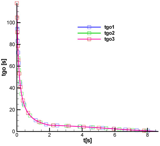
Figure 40.
Time to hit the target.
Figure 41 (detail) shows that while for nominal case 2 the evolution of the parameter is linearly decreasing towards 0 at the end, in extreme cases 1 and 3, the evolution shows jumps due to oscillations in the command parameters presented above.
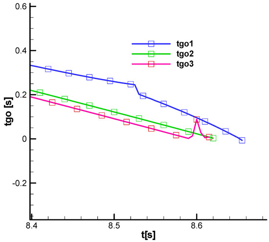
Figure 41.
Time to hit the target—detail.
11. Conclusions
Several items were covered in the analysis of the stability of the homing missile with single-channel slow rolling. Thus, in Section 2, the equations of general motion are constructed in the body frame, and in Section 3, the equations of general motion are obtained in the Resal frame. Section 4 defines the basic motion and maximum maneuver that a single-channel slow-rolling rocket with aerodynamic command can achieve. Next, in Section 5, the coupled linear form of the commanded motion of the rolling missile is obtained. Based on the symmetry of the configuration, symmetrical terms were highlighted on the two channels (pitch and yaw), as well as coupling terms as complex quantities. Based on these coupled equations, in Section 6, the flight quality parameters of the motion are highlighted, obtaining the structural scheme for the commanded motion in the case of the rolling missile. Due to the coupling of the two channels, the scheme contains complex parameters specific to this type of missile. Next, in Section 7, the guided flight model is built. For this, the kinematic equations of guidance and the equations of the target tracker, in nonlinear and linear form, are defined. Next, the actuator was analyzed, particularly the way the command is formed for the single-channel rolling missile, highlighting the phase and amplitude of the command, thus linking the guidance signal coming from the seeker to the commanded object by the complex form of the actuator. Given the specific mode of forming the command with time-modulated maximum deflection, the command switching function has been defined based on the relative roll angle obtained from summing the command phase and the current roll angle value. Given the possible errors in determining the roll angle and the imprecision in defining the advance angle in compensating the actuator response time to the relative roll angle, an additional phase shift was considered, and the analysis was carried out taking this angle into account. Based on this development, in Section 7, the guidance equations that complete the nonlinear 6-DOFs model resulted in the body frame, obtaining the model of nonlinear guided flight. On the other hand, the structural diagram of the commanded object obtained in Section 5 and the transfer functions for the kinematic guidance block of both the seeker and actuator were connected through the guidance loop, obtaining a closed-loop structural diagram of the homing missile. Within this scheme, two parameters are highlighted, namely, the time to hit the target () and the navigation constant , parameters that will be the main object of analysis in the following sections. In Section 8, we start from the established structural diagram and build the characteristic polynomial of the transfer function associated with the closed-loop scheme. Since the scheme contains complex elements (with real and imaginary parts), the characteristic polynomial obtained will also contain complex coefficients. For this reason, the Frank–Wall (F-W) criterion, equivalent to the Routh–Hurwitz (R-H) criterion, was applied to verify the stability of the system polynomials with complex coefficients. Since the obtained characteristic polynomial is of 4th order, the stability criterion defines four parameters whose values must be positive to guarantee stability. Because these parameters have complicated expressions and are difficult to handle analytically, rolling was neglected, obtaining the R-H parameters with much simpler expressions that were analyzed analytically. The analysis of the four R-H parameters resulted in four system limitations. Thus, the first condition of R-H resulted in a lower limitation , and the second condition resulted in an eventual upper limitation , depending on the values of some parameters. The third condition resulted in an upper limitation for the navigation constant , and the fourth condition imposed a lower limitation of the navigation constant. If analytical expressions were obtained for the R-H parameters that could be analyzed, the more complicated F-W parameters were solved using numerical solutions. For this, Section 9 defines a calculation model similar to a rocket of the analyzed category for which aerodynamic, mechanical, thrust, time constants and amplification constants were provided, including a value for the time to reach the target and for the navigation constant . With this model data, in Section 10, the four F-W parameters that checked the stability conditions are evaluated. At the same time, the influence of the main parameters on the location of the roots of the characteristic polynomial was evaluated. Next, the analysis was resumed but this time was performed numerically for the F-W stability parameters, identifying the two limits of the duration of hitting the target ( and the two limits for the navigation constant . The comparison of the results obtained with the two criteria (R-H and F-W) shows that the stability range obtained for the navigation constant is reduced for the case of the rolling rocket in comparison to the case of the no-rolling rocket, especially at the upper limit. In order to verify the results obtained in the linear model with the stability criterion F-W, a tactical situation was built on the fixed target with the nonlinear model in which the flight parameters and the guidance parameters were evaluated for three cases: the first case where the navigation constant was less than the minimum defined limit condition 4 of F-W, the second case where the navigation constant is similar to the value used in linear model analysis within the stability range and the third case where the navigation constant is greater than the maximum permissible value in condition 3 F-W. The results of the nonlinear model confirmed the limitations obtained with the F-W criterion. In the first and last cases, with the navigation constants out of range, the missile could not hit the target, having large oscillations in the guidance parameters (phase and fill factor) near the target. Instead, in the second case, with the navigation constant in the prescribed range, the missile hit the target, the guidance parameters having an asymptotic behavior up to the vicinity of the target. In parallel with the guidance parameters, the behavior of for the three cases was analyzed, finding that in case 1 and 3, it shows jumps in the vicinity of the target. In contrast, for case 2, it is asymptotically close to 0.
Synthesizing, the paper starts from a 6-DOFs model in the body frame from which a 6-DOFs model in the Resal frame is obtained, which is used to linearize the coupled commanded motion for the case of the slow-rolling missile. The commanded object’s structural scheme is obtained, flight quality parameters are defined, and the quantities obtained have a complex form (with real and imaginary parts) due to the coupling between longitudinal channels. Then, the kinematic guidance equation, the seeker equations and the actuator specific to the slow-rolling single-channel missile are defined by using a switching function. The guidance kinematic equations, the seeker equations, and the actuator relation are linearized in the Resal frame, and the structural diagram of the homing missile is constructed. Starting from this, the characteristic polynomial is determined, which, having complex coefficients, is analyzed with the F-W stability criterion. Based on the analysis, a stability range is determined for the navigation constant , and also the minimum limit and possibly maximum limit for the time to hit the target are obtained. The stability range defined for the navigation constant in the linear model is finally verified in the nonlinear body frame model.
Starting from the results obtained, in a future paper, we intend to analyze the stability of the slow-rotating single-channel remote-guided missiles used to combat armored vehicles.
This paper contains four Appendixes, as follows: Appendix A presents in graphical form the main terms of development of aerodynamics coefficients; Appendix B presents in graphical form the linear model flight quality parameters used for the characteristic polynomial of the transfer function; Appendix C presents in graphical form the real and imaginary part of the characteristic polynomial coefficients as well as the four stability parameters F-W; and Appendix D details the calculation of stability parameters F-W.
12. Notations
Reference Frames
—the local frame
(start frame) with the fixed origin located at sea level, where the axis is in a
conveniently chosen direction, and the axis is oriented
vertically upwards. The local frame is considered an inertial frame.
—the mobile
ground frame, with a movable origin, is located at the missile’s center of
mass. Its axes are parallel to those of the local frame, but the axis is oriented
vertically downwards. The mobile ground frame is considered an inertial frame.
—the body frame
with the mobile origin is situated at the missile’s center of mass. The axis coincides with
the configuration’s axis of symmetry, pointing towards the missile’s top. The
axes and are in the
configuration’s symmetry planes. The body frame is considered a non-inertial
frame.
—the Resal frame
is a quasi-linked body frame that does not participate in its roll motion.
Author Contributions
Conceptualization, T.-V.C.; Methodology, T.-V.C.; Software, T.-V.C.; Validation, T.-V.C., C.E.C., V.P. and A.C.; Formal analysis, T.-V.C., C.E.C., V.P. and C.E.; Investigation, T.-V.C.; Resources, T.-V.C.; Data curation, T.-V.C.; Writing—original draft, T.-V.C., C.E.C., V.P., C.E. and A.C.; Writing—review & editing, T.-V.C., C.E.C., V.P., C.E. and A.C.; Visualization, T.-V.C., C.E.C., V.P., C.E. and A.C.; Supervision, T.-V.C.; Project administration, T.-V.C. All authors have read and agreed to the published version of the manuscript.
Funding
This research received no external funding.
Data Availability Statement
The original contributions presented in the study are included in the article, further inquiries can be directed to the corresponding authors.
Conflicts of Interest
The authors declare no conflict of interest.
Abbreviations
The Equation of Movement Parameters
—the components of velocity in the body frame;
—the components of the rotation velocity in the body frame;
—the dimensionless components of the rotational velocity in the body frame;
—yaw angle; —pitch angle; —roll angle;
—angle of incidence (attack angle) in the pitch plane; —angle of incidence (attack angle) in the yaw plane;
—the dimensionless unsteady incidences;
—mass;
—angular momentum;
—aerodynamic force;
—aerodynamic torque;
—thrust;
—gasodynamic torque;
—weight;
—gravitational acceleration;
—the components of velocity in Resal frame;
—the components of the rotational velocity in Resal frame;
—the dimensionless components of the rotational velocity in Resal frame;
—the velocity of rotation of the body frame connected to the rocket in relation to the Resal frame.
The Flight Quality Parameters
—the natural pulsation of nutation;
—the damping factor of nutation;
—the time constant of nutation;
—the command factor;
—the advance time on command;
the angular rate of precession;
—the static stability;
—the reference time;
the reduced mass of the aircraft or relative density;
—the reduced moment of inertia in pitch;
—the reduced gravitational acceleration;
—the maximum load factor.
The Guidance Parameters
—the attitude angles for the guiding frame orientation;
—line of sight (LOS);
—range;
, —absolute angles of the line of sight;
—missile aspect angles;
—target aspect angles;
—missile climb angle and flight path azimuth angle;
—target climb angle and flight path azimuth angle;
—missile velocity;
—the components of the missile velocity in the guiding frame;
, —the projections of the missile velocity in the first and the second guiding plane, respectively;
—target velocity;
—the components of the target velocity in the guiding frame;
, —the projections of the target velocity in the first and the second guiding plane, respectively;
—missile acceleration;
—the components of the missile acceleration in the guiding frame;
—target acceleration;
—the components of the target acceleration in the guiding frame;
, —angular rate of LOS;
—missile angular rates of the velocity vector;
—target angular rates of the velocity vector;
—proportional navigation constant (gain);
—modified proportional navigation constant (gain);
—time to go;
—the collision velocity;
—the guidance command in body frame;
—the guidance command in Resal frame;
—the command module;
—the command phase;
—the phase shift error;
—the fill factor;
the relative roll angle;
—the pitch canard deflection angle;
—the average equivalent canard deflection;
—the seeker gain;
—the seeker time constant;
—the actuator gain.
Appendix A. Aerodynamics
The aerodynamic coefficients are obtained in the body frame.
The reference surface for all coefficients is the cross-section of the fuselage.
The reference length used for torque coefficients is the length of the fuselage.
The momentum coefficients were related to the final position of the rocket’s center of mass without fuel.
The main terms in the development of the presented aerodynamic coefficients were obtained according to the work [26] and corrected by dedicated experimental results in the wind tunnel.

Figure A1.
Term of axial force coefficient at zero incidence.
Figure A1.
Term of axial force coefficient at zero incidence.


Figure A2.
Terms of development of the coefficient of axial force with squares of incidences.
Figure A2.
Terms of development of the coefficient of axial force with squares of incidences.


Figure A3.
The term of development of the coefficient of axial force with the square of the canard angular deflection.
Figure A3.
The term of development of the coefficient of axial force with the square of the canard angular deflection.


Figure A4.
Terms of development of coefficients of normal forces with incidences.
Figure A4.
Terms of development of coefficients of normal forces with incidences.


Figure A5.
Terms of development of coefficients of normal forces with incidence cube.
Figure A5.
Terms of development of coefficients of normal forces with incidence cube.


Figure A6.
Terms of development of normal force coefficients with angular canard deflection.
Figure A6.
Terms of development of normal force coefficients with angular canard deflection.


Figure A7.
Terms of development of the torque coefficients in pitch and yaw with incidences.
Figure A7.
Terms of development of the torque coefficients in pitch and yaw with incidences.


Figure A8.
Terms of development of pitch and yaw torque coefficients with incidence cube.
Figure A8.
Terms of development of pitch and yaw torque coefficients with incidence cube.


Figure A9.
Terms of development of the torque coefficient in pitch with angular canard deflection.
Figure A9.
Terms of development of the torque coefficient in pitch with angular canard deflection.


Figure A10.
Terms of development of the roll torque coefficient.
Figure A10.
Terms of development of the roll torque coefficient.

Non-stationary and rotational terms, including Magnus terms, were determined using apparent mass theory from the work [26].
Appendix B
Appendix B.1. Basic Movement

Figure A11.
Equilibrium incidence.
Figure A11.
Equilibrium incidence.


Figure A12.
Equilibrium angular canard deflection.
Figure A12.
Equilibrium angular canard deflection.

Appendix B.2. Stability Matrix

Figure A13.
Derivative term of incidence equation against incidence.
Figure A13.
Derivative term of incidence equation against incidence.


Figure A14.
Derivative term of incidence equation against angular velocity.
Figure A14.
Derivative term of incidence equation against angular velocity.


Figure A15.
Derivative term of incidence equation against unsteady incidence.
Figure A15.
Derivative term of incidence equation against unsteady incidence.


Figure A16.
Derivative term of incidence equation against cross-incidence—Magnus term.
Figure A16.
Derivative term of incidence equation against cross-incidence—Magnus term.


Figure A17.
Derivative term of incidence equation against cross-angular velocity—Magnus term.
Figure A17.
Derivative term of incidence equation against cross-angular velocity—Magnus term.


Figure A18.
Derivative term of angular velocity equation against incidence.
Figure A18.
Derivative term of angular velocity equation against incidence.


Figure A19.
Derivative term of angular velocity equation against angular velocity.
Figure A19.
Derivative term of angular velocity equation against angular velocity.


Figure A20.
Derivative term of angular velocity equation against unsteady incidence.
Figure A20.
Derivative term of angular velocity equation against unsteady incidence.


Figure A21.
Derivative term of angular velocity equation against cross-incidence—Magnus term.
Figure A21.
Derivative term of angular velocity equation against cross-incidence—Magnus term.


Figure A22.
Derivative term of angular velocity equation against cross-angular velocity—Magnus and gyroscopic term.
Figure A22.
Derivative term of angular velocity equation against cross-angular velocity—Magnus and gyroscopic term.

Appendix B.3. Command Matrix

Figure A23.
Derivative term of incidence equation against canard deflection.
Figure A23.
Derivative term of incidence equation against canard deflection.


Figure A24.
Derivative term of angular velocity equation against canard deflection.
Figure A24.
Derivative term of angular velocity equation against canard deflection.

Appendix B.4. Flight Quality Parameters

Figure A25.
Static stability.
Figure A25.
Static stability.


Figure A26.
Natural pulsation of nutation.
Figure A26.
Natural pulsation of nutation.


Figure A27.
Nutation damping factor.
Figure A27.
Nutation damping factor.


Figure A28.
Command factor.
Figure A28.
Command factor.


Figure A29.
The time constant of the missile.
Figure A29.
The time constant of the missile.


Figure A30.
Maximum load factor.
Figure A30.
Maximum load factor.

Appendix C
Appendix C.1. Coefficients of the Characteristic Polynomial: i—Initial; f—Final

Figure A31.
Coefficient of the cubic term—the real part.
Figure A31.
Coefficient of the cubic term—the real part.


Figure A32.
Coefficient of the quadratic term—the real part.
Figure A32.
Coefficient of the quadratic term—the real part.


Figure A33.
Coefficient of the term of the first order—the real part.
Figure A33.
Coefficient of the term of the first order—the real part.


Figure A34.
Free-term coefficient—the real part.
Figure A34.
Free-term coefficient—the real part.


Figure A35.
Coefficient of the cubic term—the imaginary part.
Figure A35.
Coefficient of the cubic term—the imaginary part.


Figure A36.
The coefficient of the term square—the imaginary part.
Figure A36.
The coefficient of the term square—the imaginary part.


Figure A37.
Coefficient of the term of the first order—the imaginary part.
Figure A37.
Coefficient of the term of the first order—the imaginary part.


Figure A38.
Free-term coefficient—the imaginary part.
Figure A38.
Free-term coefficient—the imaginary part.

Appendix C.2. Stability Parameters F-W: i-Initial; f- Final

Figure A39.
First parameter F-W.
Figure A39.
First parameter F-W.


Figure A40.
Second parameter F-W.
Figure A40.
Second parameter F-W.


Figure A41.
Third parameter F-W.
Figure A41.
Third parameter F-W.


Figure A42.
Fourth parameter F-W.
Figure A42.
Fourth parameter F-W.

Appendix D. Frank–Wall Stability Criterion for the 4th-Order Polynomial
Let the polynomial of order 4 with complex coefficients be the following:
In order to verify that the real part of the roots is negative, according to [16], an associated polynomial of the form is constructed:
After which, the ratio of the polynomials is put into the following form:
The stability condition of F-W is formulated by two theorems in the paper [16].
The first theorem shows that for the polynomial of order (A 1), with complex coefficients, to have all its roots on the negative real side, it is necessary and sufficient that and that be pure complex numbers or null.
The second theorem shows that the polynomial of order , with complex coefficients, has as many roots on the positive real side as values are negative.
In the same work, an algorithm for obtaining parameters , is indicated, which will be briefly presented below.
Thus, the coefficients of the two polynomials are denoted by the following:
After which, for the 4th-order polynomial, the following is obtained successively:
Based on these intermediate parameters, the parameters of interest can be determined:
respectively,
Based on the algorithm described above, for the 4th-order polynomial, the following expressions were obtained:
where it was denoted by the following:
Hence, the following:
From the previous relation, it is observed that are pure complex numbers in all cases, which, according to the values and may be null. The only conditions to be verified or imposed are that .
Check for Non-Rolling Case
For the case without rotation, the four parameters become
Which leads to the following stability conditions:
On the other hand, the Routh–Hurwitz conditions for the 4th-order polynomial with real coefficients are obtained from the matrix of coefficients constructed as follows:
The condition is that all determinants in the table are positive.
In this case, it is as follows:
The conditions are identical to the conditions of F-W (A12) for the case of real coefficients.
References
- Hu, X.; Yang, S. Coning motion instability of spinning missiles induced by the delay of strap-down seeker. Chin. J. Aeronaut. 2021, 33, 3360–3368. [Google Scholar] [CrossRef]
- Hu, S.; Wang, J.; Wang, Y.; Tian, S. Stability Limits for the Velocity Orientation Autopilot of Rolling Missiles. IEEE Access 2021, 9, 110940–110951. [Google Scholar] [CrossRef]
- Hu, X.; Yang, S.; Xiong, F.; Zhang, G. Stability of spinning missile with homing proportional guidance law. Aerosp. Sci. Technol. 2017, 71, 546–555. [Google Scholar] [CrossRef]
- Suiçmez, E.C.; Kutay, A.T. Single channel digital controller design for a high spinning rate rolling airframe missile. Aeronaut. J. 2022, 126, 1815–1833. [Google Scholar] [CrossRef]
- Karimi, J. A new closed form solution for dynamic stability analysis of rolling airframes having one pair on-off actuator. Aviat. Open Access 2021, 25, 92–103. [Google Scholar] [CrossRef]
- Botez, R.M.; Chelaru, V.; Parvu, P.; Gheorghe, C. Calculus model for a rolling guided missile. J. Vib. Control. 2001, 7, 863–889. [Google Scholar] [CrossRef]
- Chelaru, T.-V.; Constantinescu, C.E. Theoretical and experimental solutions for multistage quasi-guided rocket. In Proceedings of the International Astronautical Congress, IAC, Washington, DC, USA, 21–25 October 2019. [Google Scholar]
- Zheng, Q.; Zhou, Z. Flight Stability of Canard-Guided Dual-Spin Projectiles with Angular Rate Loops. Int. J. Aerosp. Eng. 2020, 2020, 2705175. [Google Scholar] [CrossRef]
- Zheng, D.; Lin, D.; Wang, J.; Xu, X. Dynamic stability of rolling missiles employing a two-loop autopilot with consideration for the radome aberration parasitic feedback loop. Aerosp. Sci. Technol. 2017, 61, 1–10. [Google Scholar] [CrossRef]
- Tian, S.; Lin, D.; Wang, J.; Li, B. Dynamic stability of rolling missiles with angle-of-attack feedback three-loop autopilot considering parasitic effect. Aerosp. Sci. Technol. 2017, 71, 592–602. [Google Scholar] [CrossRef]
- Zheng, D.; Lin, D.; Xu, X.; Tian, S. Dynamic stability of rolling missile with proportional navigation & PI autopilot considering parasitic radome loop. Aerosp. Sci. Technol. 2017, 67, 41–48. [Google Scholar]
- Qin, S.-J.; Zhang, F.-X. A Combination of Silicon Micro-gyroscope that Application Rotary Missile Attitude Control System. In Proceedings of the 2011 International Conference on Physics Science and Technology (Icpst), Hong Kong, China, 28–30 December 2011. [Google Scholar]
- Yan, X.; Chen, G.; Tian, X. Two-Step Adaptive Augmented Unscented Kalman Filter for Roll Angles of Spinning Missiles Based on Magnetometer Measurements. Meas. Control. 2018, 51, 73–82. [Google Scholar] [CrossRef]
- Jahangir, E.; Howe, R.M. Time-Optimal Attitude Control Scheme for a Spinning Missile. J. Guid. Control. Dyn. 1993, 16, 346–353. [Google Scholar] [CrossRef][Green Version]
- Kocetkov, V.T.; Polovko, A.M.; Ponomarev, B.M. Theory of Self-Guided and Remote-Controlled Missile Systems; Nauka: Moskva, Russian, 1964. [Google Scholar]
- Frank, E. On the zeros of polynomials with complex coefficients. Bull. Amer. Math. Soc. 1946, 52, 144–157. [Google Scholar] [CrossRef]
- ISO 1151-75; Flight Dynamics—Concepts, Quantities and Symbols—Part 5: Quantities Used in Measurements. ISO: Geneva, Switzerland, 1987.
- STP M 40406-99; The Commanded Missile System—Terminology and Symbols. Ministry of National Defence (MoND): Bucharest, Romania, 1998.
- Niţă, M.M.; Andreescu, D. ŞT. Rocket Flight; Militara: Bucharest, Romania, 1964. [Google Scholar]
- Chelaru, T.V. Dynamics of Flight—Guided Missile, 2nd ed.; Revised and Added; Printech: Bucharest, Romania, 2004; p. 434. [Google Scholar]
- Kuzovkov, N.T. Flight Stabilization Systems, Ballistic Missile and Anti-Aircraft Missile; Visaia Skola: Moskva, Russian, 1976. [Google Scholar]
- Belea, C.; Lungu, R.; Cismaru, C. Gyroscopic Systems and Their Applications; Scrisul Romanesc: Craiova, Romania, 1986. [Google Scholar]
- Hacker, T. Stability and Control in Flight Theory; Romanian Academy: Bucharest, Romania, 1968. [Google Scholar]
- STP M 40455-99; The Guided Missile System—Terminology and Symbols. Ministry of National Defence (MoND): Bucharest, Romania, 1998.
- Carpantier, R. Guidance des Avions et des Missiles Aerodynamiques; Tom I,II,III, lit; ENSAE: Paris, France, 1989. [Google Scholar]
- Nielsen, J. Missile Aerodynamics; McGraw-Hill Book Company, Inc.: New York, NY, USA; Toronto, ON, Canada; London, UK, 1960. [Google Scholar]
- Sviatoduh, V. Dynamics of Spatial Motion of Guided Missiles; Masinostroenie: Moskva, Russian, 1969. [Google Scholar]
- Ben-Asher, J.Z.; Isaac, Y. Advanced in Missile Guidance Theory; American Institute of Aernautics and Astronautics: Preston, VA, USA, 1998. [Google Scholar]


Disclaimer/Publisher’s Note: The statements, opinions and data contained in all publications are solely those of the individual author(s) and contributor(s) and not of MDPI and/or the editor(s). MDPI and/or the editor(s) disclaim responsibility for any injury to people or property resulting from any ideas, methods, instructions or products referred to in the content. |
© 2024 by the authors. Licensee MDPI, Basel, Switzerland. This article is an open access article distributed under the terms and conditions of the Creative Commons Attribution (CC BY) license (https://creativecommons.org/licenses/by/4.0/).