Article

Rutting Caused by Grouser Wheel of Planetary Rover in Single-Wheel Testbed: LiDAR Topographic Scanning and Analysis

1
The Space Robotics Laboratory (SRL) in Department of Aerospace Engineering, Tohoku University, Aoba 6-6-01, Sendai 980-8579, Miyagi, Japan
2
Advanced Robotics Laboratory (AdRoLab) in School of Electrical and Computer Engineering, State University of Campinas, Campinas 13083-852, São Paulo, Brazil
*
Authors to whom correspondence should be addressed.
These authors contributed equally to this work.
Aerospace 2025, 12(1), 71; https://doi.org/10.3390/aerospace12010071
Submission received: 18 October 2024 / Revised: 9 December 2024 / Accepted: 12 December 2024 / Published: 20 January 2025
(This article belongs to the Special Issue Planetary Exploration)

Abstract

:
This paper presents datasets and analyses of 3D LiDAR scans capturing the rutting behavior of a rover wheel in a single-wheel terramechanics testbed. The data were acquired using a LiDAR sensor to record the terrain deformation caused by the wheel’s passage through a Toyoura sandbed, which mimics lunar regolith. Vertical loads of 25 N, 40 N, and 65 N were applied to study how rutting patterns change, focusing on rut amplitude, height, and inclination. This study emphasizes the extraction and processing of terrain profiles from noisy point cloud data, using methods like curve fitting and moving averages to capture the ruts’ geometric characteristics. A sine wave model, adjusted for translation, scaling, and inclination, was fitted to describe the wheel-induced wave-like patterns. It was found that the mean height of the terrain increases after the grouser wheel passes over it, forming ruts that slope downward, likely due to the transition from static to dynamic sinkage. Both the rut depth at the end of the wheel’s path and the incline increased with larger loads. These findings contribute to understanding wheel–terrain interactions and provide a reference for validating and calibrating models and simulations. The dataset from this study is made available to the scientific community.

1. Introduction

Planetary rovers are critical for advancing space exploration, enabling the study of distant terrains and the collection of valuable data. Among the many challenges they face, traversing the Moon’s surface poses significant difficulties. The lunar surface is almost entirely covered by a layer of fine-grained debris known as regolith, which forms through continuous impact cratering and space weathering [1]. Its thickness is estimated to be 10 m in the highlands and 5 m in the mare [2]. Beneath this surface layer, lunar regolith reveals a complex structure, transitioning from fine grains to coarser particles interspersed with larger rock fragments [3]. Understanding these properties is critical for rover design, as the fine-grained characteristics of regolith cause rovers to slip, sink, and potentially become permanently embedded in the soil.
A key challenge in rover operations is mitigating wheel slip, which increases energy consumption and can hinder mobility and compromise mission success [4]. Addressing this issue involves slip estimation and compensation through control systems. Slip estimation techniques typically rely on internal sensors or cameras. In particular, analyzing ruts left by wheels has emerged as a promising method for quantifying slip and understanding terrain interactions [5].
Simulations have become essential tools in planetary mobility research, enabling the replication of wheel–soil dynamics and rutting patterns. Models based on terramechanics principles and discrete element methods (DEMs) allow researchers to study and validate rover performance under simulated conditions. However, these simulations require calibration and validation, which can be performed using data from terramechanics test rigs or field tests.
Single-wheel testbeds (SWTs), also known as soil bins, are widely used in terramechanics research to study wheel-induced terrain deformation. These setups typically consist of a prepared soil bin and a drive unit that moves a wheel under controlled conditions, enabling detailed analyses of terrain deformation caused by different wheel designs and loading scenarios [6]. Advanced sensing technologies, such as LiDAR (Light Detection and Ranging), have further enhanced these studies. Introduced in the 1960s [7], LiDAR provides high-resolution, three-dimensional terrain data through laser pulses. Its ability to capture detailed profiles independent of lighting conditions has made it indispensable for both controlled testbeds and extraterrestrial environments like the Moon or Mars. However, LiDAR can suffer from some sources of innacuracies, which are discussed in Section 2. By combining SWTs with LiDAR, researchers can precisely measure and analyze deformations such as ruts, enabling better calibration of simulation models and improving rover mobility.
This study integrates LiDAR technology with an SWT to investigate the rutting behavior caused by grouser wheels. Specifically, it introduces two methodological innovations: (1) employing LiDAR to capture high-resolution data on wheel-induced terrain deformation and (2) analyzing these deformations by modeling the resulting ruts as curve-fitted sine waves to extract dimensional characteristics. By making the resulting datasets publicly available, this work aims to support the development of advanced simulation and navigation models for planetary exploration.

1.1. Relevance

The ruts left by grouser wheels (see Figure 1) are directly linked to the rover’s interaction with the terrain, providing valuable data that can be used to estimate driving states. For instance, the spacing and pattern of these traces reflect real-time slip conditions, which are important for rover localization and control systems. Saku and Ishigami [8] have demonstrated the use of machine learning to estimate slip based on the spacing of ruts in an SWT. Similarly, Reina et al. [9] have developed a vision-based method to estimate side-slip angles based on images of ruts from a rover-mounted rear camera in field tests. These methods enable more efficient movement and navigation in planetary environments.
The depth of ruts has implications for rover mobility as it is linked to the sinkage of the wheel. The sinkage of the wheel, in turn, increases with the load and slip ratios. When wheel sinkage or the slip ratio is high, this represents lower energy efficiency and a higher risk of entrapment. Gao et al. [10] conducted experiments to determine tractive efficiency on sandy soil and found it to increase to a maximum when the slip ratio was around 15% and then decrease.
In this study, a LiDAR sensor is integrated into an SWT setup. Future studies could explore mounting a LiDAR sensor on a rover for terrestrial field experiments or planetary missions. Inspired by Ding [11], who described the first rover-mounted ground-penetrating radar used in the Chang’E-3 mission, a downward-facing LiDAR could capture terrain deformations caused by rover wheels. Such scans could be utilized to estimate wheel slippage and sinkage and the bearing capacity of regolith.
The development of a rover’s traction and navigation systems depends on simulation frameworks. The inclusion of wheel ruts in these simulations increases their fidelity for vision-based tasks. The relevance of ruts is underscored by their inclusion in lunar and Martian simulators, as referenced in works such as [12,13,14,15,16,17]. A vision-based navigation system could use terrain deformations as landmarks for SLAM (Simultaneous Localization and Mapping), improving navigation in feature-sparse terrains.

1.2. Contributions

The primary contributions of this study are
  • Employing LiDAR technology to characterize wheel-induced terrain deformation in a SWT.
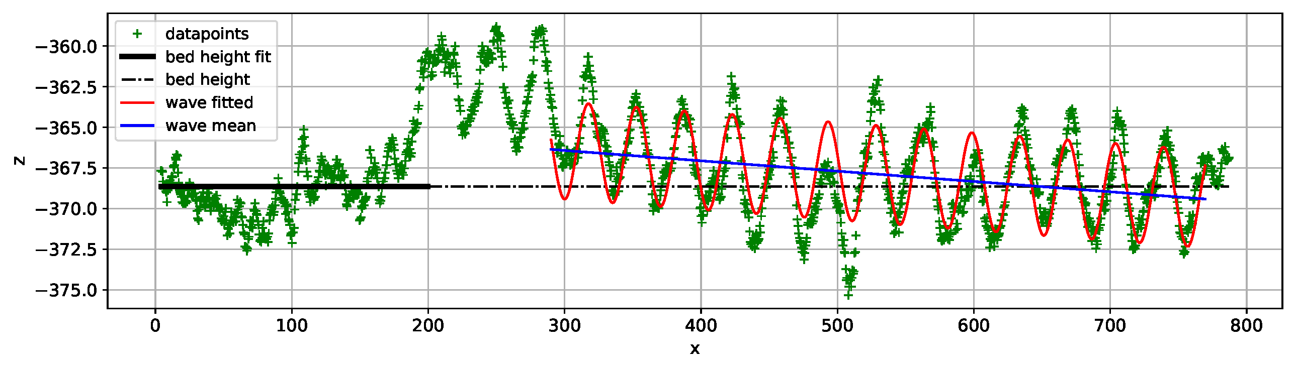
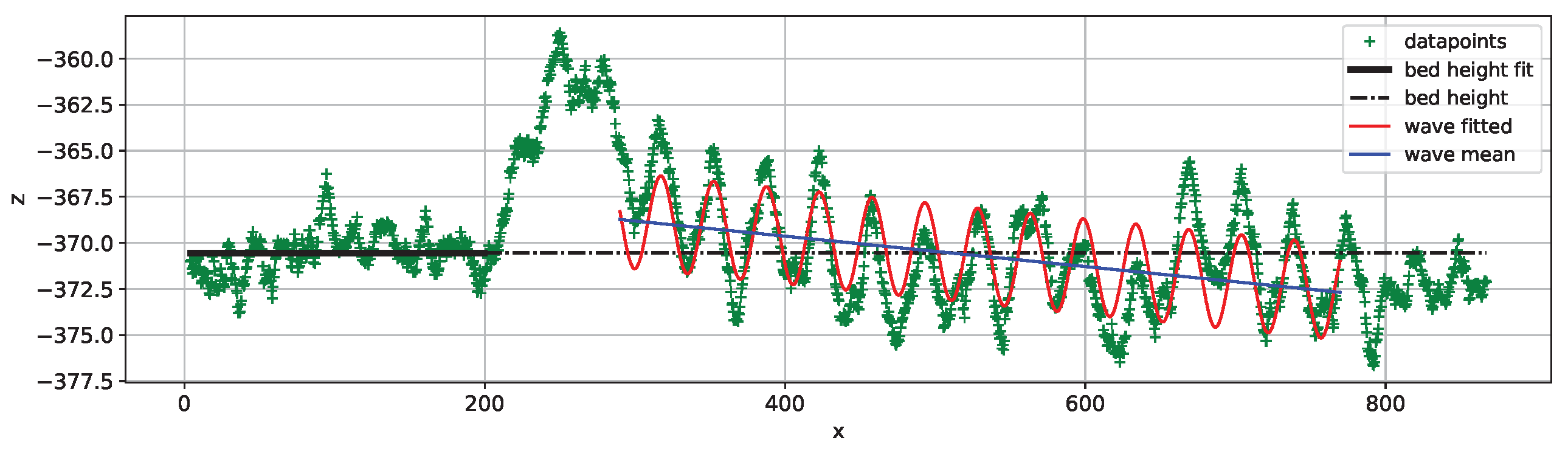
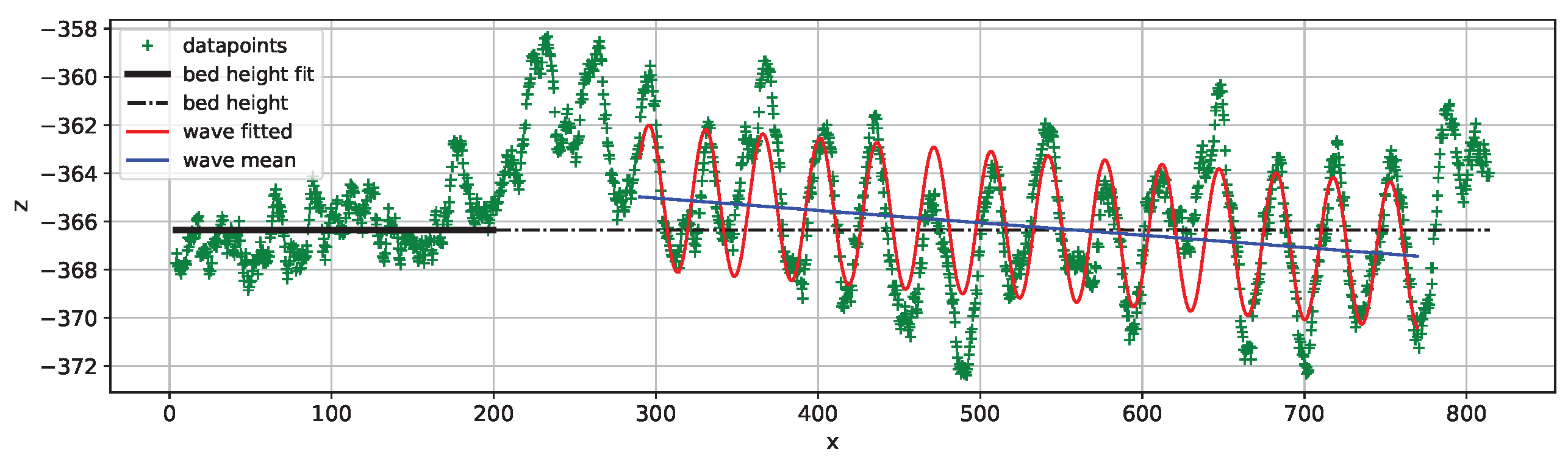
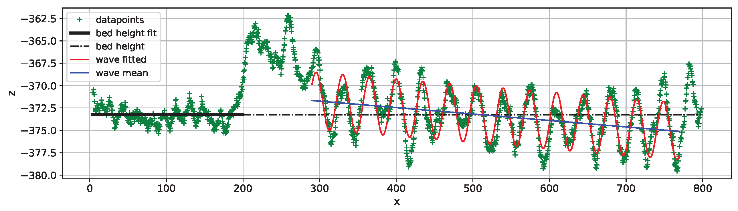
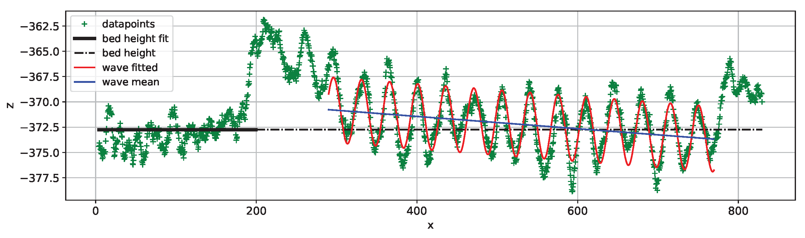
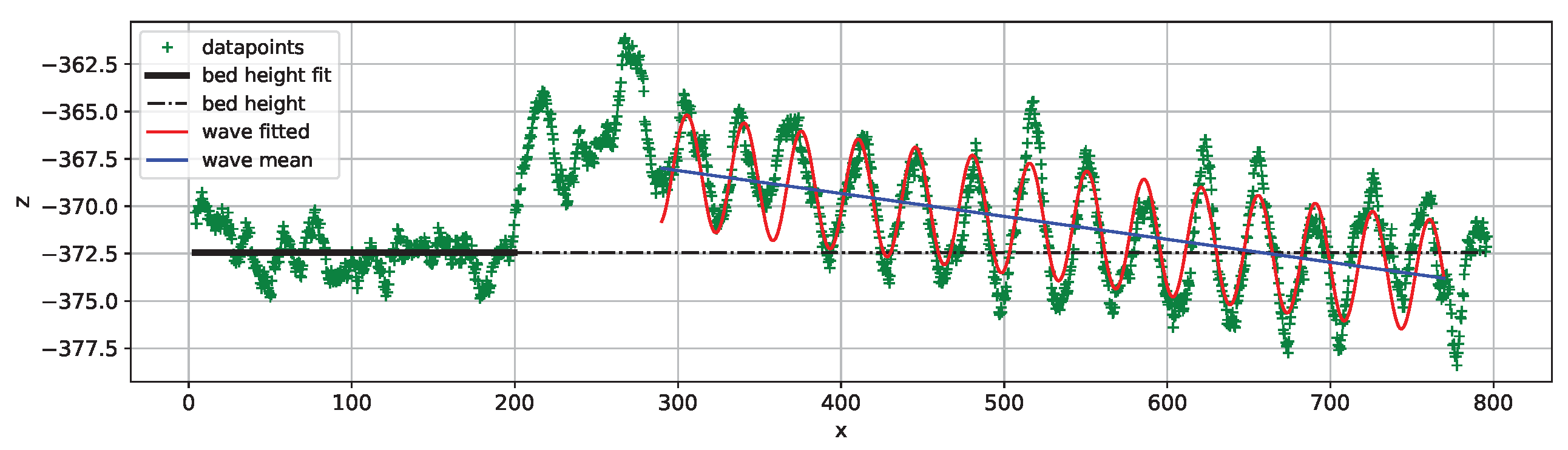
  • Modeling ruts using curve-fitted sine waves to extract their average dimensions.
By making the datasets publicly accessible, this research supports future efforts in terramechanics, rover mobility studies, and simulation development.

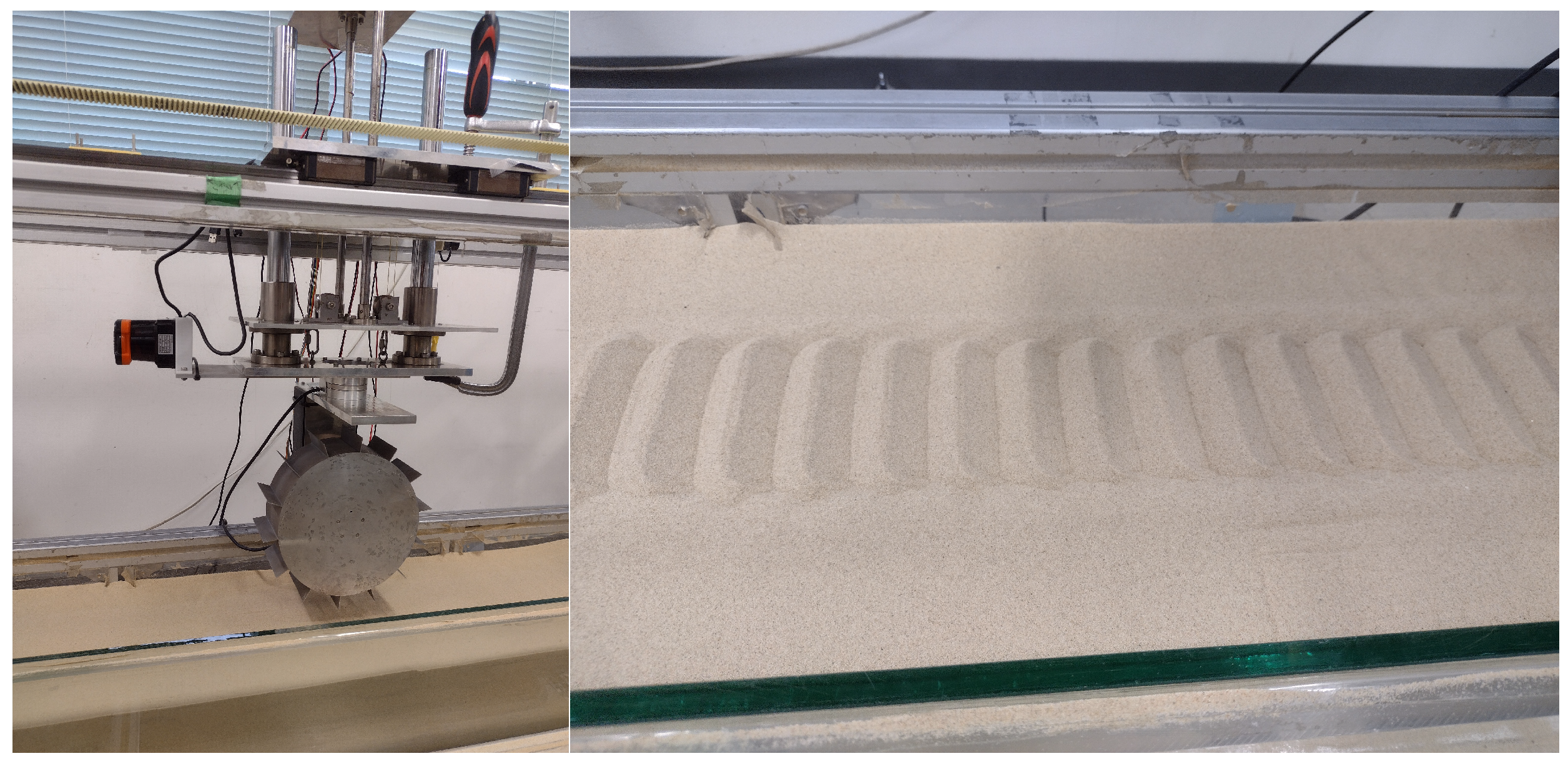
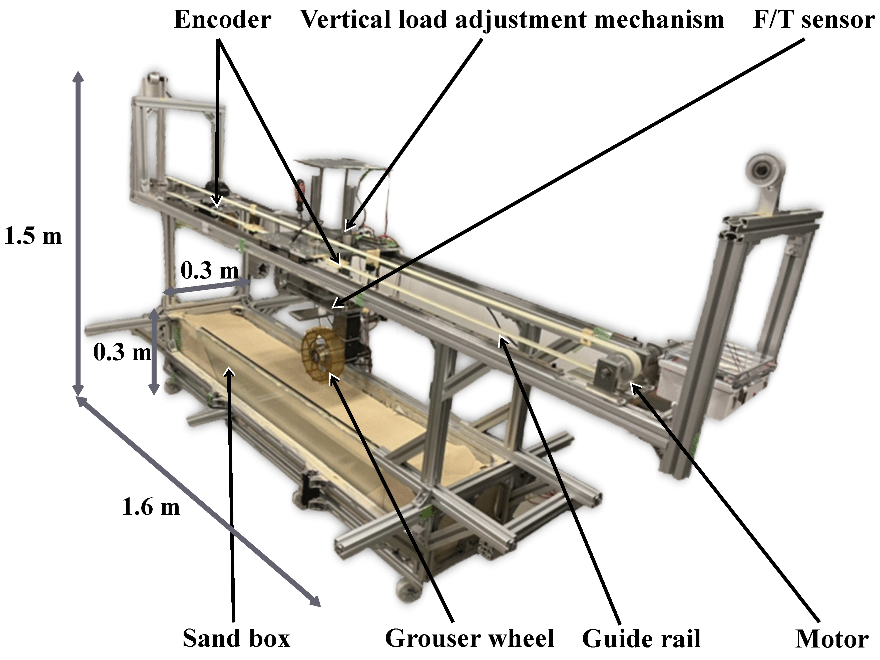
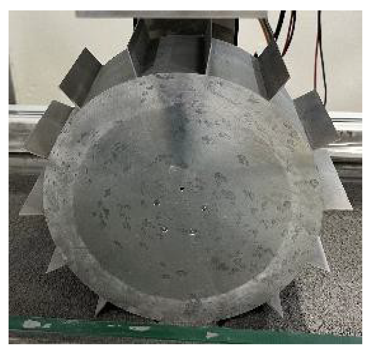
2. Experimental Description

The single-wheel testbed employed in the experiments was developed by our research group [18]. It has a length of 2.5 m, a width of 0.3 m, and a height of 1.5 m, and it is shown in Figure 2. It is composed of (1) a wheel drive unit equiped with a force/torque (F/T) sensor, (2) a passive vertical moving unit that supports the wheel drive unit, (3) a translational drive unit which runs along the guide rail, and (4) a sandbox.
The LiDAR sensor used is the Hokuyo UST-30LX scanning laser range finder (HOKUYO AUTOMATIC CO., LTD, Osaka, Japan). It has been integrated into SWTs during previous studies due to its compatibility with the testbed setup. LiDAR systems, however, are prone to various sources of errors. In our indoor setup, where the LiDAR is mounted on a cart moving along prismatic guides at a close distance of 30 cm from the target, many error types commonly associated with outdoor or aerial scanning—such as IMU attitude errors, boresight misalignment, vegetation- and snow-induced errors, environmental factors, and multiple scattering—are negligible.
For our setup, six potential error sources could influence our experiments: laser scanning errors, positioning errors, lever arm offsets, terrain characteristics, target characteristics, and system calibration errors. Laser scanning errors stem from sensor limitations, including inaccuracies in time-of-flight measurements due to the clock circuit, angular inaccuracies from the resolution of encoders inside the sensor, and beam divergence. Positioning errors arise from the SWT encoder accuracy in moving the cart along the x-direction. Lever arm offsets, caused by mismatches between the encoder’s zero point and the LiDAR’s attachment position, are irrelevant in our setup since we carried out measurements relatively, not absolutely.
Terrain slope could influence range measurements due to beam spread, but this is minimal given the short measurement distance. Target characteristics such as reflectivity and surface texture may weaken return signals, but the sensor’s capability of measuring at a range of up to 25 meters ensures strong returns at 30 cm. System calibration errors, which involve systematic deviations in angles and distances, can be mitigated by manufacturer calibrations or by the user employing reference targets at known positions and applying compensation factors to adjust the output values.
Soil called Toyoura Silica Sand [20] (Toyoura Keiseki Kogyo Co., Ltd., Shimonoseki, Yamaguchi, Japan) was used for its availability and for being known to have a low cohesion value and narrow size distribution, with a similar average particle size to lunar regolith. The mechanical properties of the soil are presented in Table 1.
We use a model wheel of the Rashid rover [23], designed for the Emirates lunar mission to explore the Atlas crater. The model wheel is made of aluminum, with a diameter of 200 mm, a width of 80 mm, and 14 grousers with lengths of 20 mm and weights of 1.18 kg. This can be seen in Figure 3. In the wheel–soil interaction, before the wheel starts to drive, it already sinks to a certain extent due to the vertical load applied. This sinking distance is referred to as static sinkage. When driving commences from this state, the wheel’s rotation scrapes away the sand, causing the wheel to sink even deeper, which is known as dynamic sinkage.
The LiDAR sensor is mounted on the wheel unit that is subject to vertical displacement due to wheel sinkage during track creation. As a result, simultaneous LiDAR measurements during the initial track creation run are not feasible, as the changing height of the LiDAR sensor introduces errors. To address this, the wheel is driven across the sandbed twice. Measurements are taken during the second pass, where the wheel is not in contact with the sand, thereby avoiding vertical displacement of the LiDAR sensor and ensuring accurate data acquisition.
The experimental procedure for acquiring LiDAR data on wheel tracks on a sandbed is as follows:
  • Terrain preparation: the sandbed is plowed to establish a loose state and is then leveled to ensure a consistent starting surface for the experiment.
  • Initial setup: the wheel unit is positioned at the starting point, and the wheel is lowered until it makes contact with the sand surface.
  • Track creation: the running parameters (rotational and horizontal velocities) are set, and the wheel is driven forward for the first time across the sandbed to create tracks.
  • Locking the wheel up: with the help of a clamp, the wheel unit is locked in the up position so it does not disturb the created tracks.
  • Cart returning: after completing the first run, the wheel unit is returned to the starting point.
  • LiDAR data acquisition: in the second forward movement, the LiDAR sensor is activated, the horizontal velocity is set, and the cart performs the movement while recording LiDAR data.
  • Repetition: the sandbed is reset to the initial conditions, and the experiment is repeated as required.

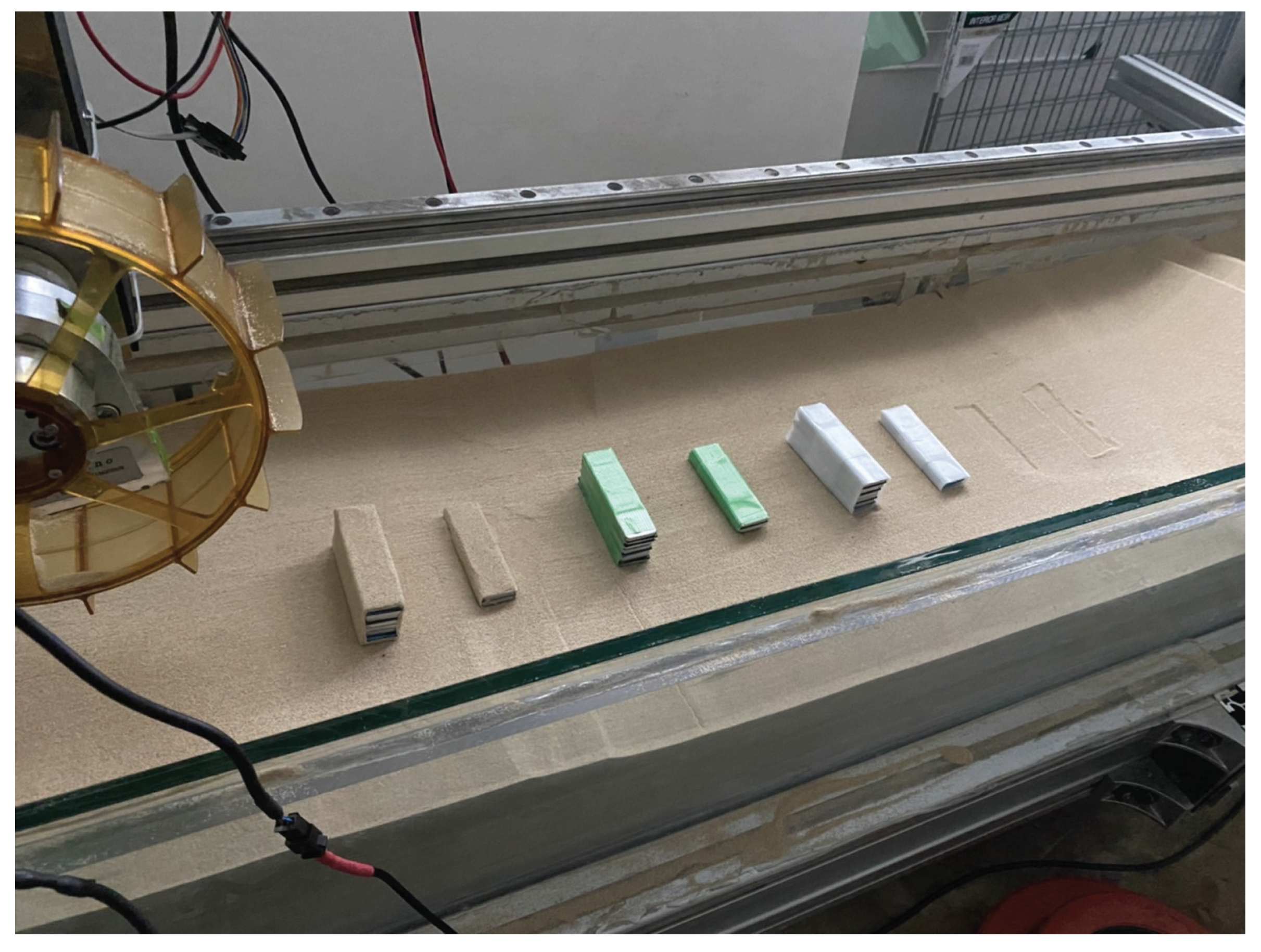
LiDAR Accuracy Experiment

An experiment was performed to determine the precision of LiDAR scanning in our test setup. The experiment involves objects of 2 different heights: big, 30 mm, and small, 10 mm. The objects have 3 types of external surfaces, covered with sand, green tape, and white tape. The experiment is shown in Figure 4.
The scan obtained from the experiment is shown in Figure 5. In this plot, intervals were selected for calculating the mean height of each object as well as for the support surface on the left and right of each object; those mean heights are shown as black lines. By subtracting the mean height of each object from the height of the sandbed on the left and right sides, it was possible to calculate the relative height of each object, which is presented in Table 2.
For this study, the accuracy of measuring the objects covered in sand was more important than for the other objects because they more closely resemble the experiment for measuring the heights of the ruts’ wave patterns. In this case, the greatest deviation found was 3.20 mm. Knowing the maximum deviation for sand-covered objects, we assume that the measurements of wheel rut waves could have deviations of up to 3.20 mm as well. The green-taped objects presented bigger errors of up to 4.16 mm. The white-taped objects presented the worst results, as the LiDAR sensor completely failed to capture the small 10 mm object.

3. Datasets

In the single-wheel testbed (SWT) with the mounted LiDAR sensor, it was possible to collect height data from the terrain after the wheel had generated a trace. However, the data from the LiDAR sensor present considerable noise, which makes it difficult to observe the characteristic wave pattern of a wheel trace. In order to filter out the noise, a moving average was applied. The number of data points to be averaged is a parameter of the moving average that needs to be tweaked to be able to filter out only the noise and not the wheel trace itself. An appropriate value of 15 was determined manually, as can be seen in Figure 6, which shows 3 to be too low and 50 to be too high.
Height data were collected for three values of vertical load—25, 40, and 65 Newtons—with a horizontal velocity of 16 mm/s and an angular velocity of 0.2 rad/s, resulting in a slip ratio of 20%. For each load, the experiment was run three times, generating a total of 9 data recordings. The plots corresponding to the recordings are presented in Figure 7, showing both the original data and those processed by a moving average of 15 data points. This dataset is publicly available and can be downloaded at https://github.com/viniciusares/wheelruts-lidar (accessed on 17 October 2024).

4. Data Analysis Methods

The LiDAR measurements do not provide absolute values. While the amplitudes of the traces are less than 10 mm, the direct measurements of the heights at any given point hover around negative 300 mm. So, it is necessary, firstly, to obtain the height of the sandbed in order to serve as a reference to then measure the heights of the wavy pattern. When the wheel is lowered to the sand in the leftmost position of the cart, there is a region of sand that remains untouched by the wheel, and this is recorded by the LiDAR sensor. The untouched region ranges from approximately 0 to 200 mm in the x-direction.
Before each test run, the sandbed was plown and then flattened using a scraping tool. The scraping tool has a shape that allows it to rest on the edges of the sandbox so that when the scraper is moved in the x-direction, it preserves the horizontality of the edges of the sandbox. Knowing that the sandbed was expected to be horizontal, a horizontal line was fitted to the data points to extract the height of the undisturbed sandbed for each test run in the region x = [0, 200] mm. The fitting of a horizontal line is equivalent to simply calculating the arithmetic mean of the data points. The bed height for each test run is presented in Table 3.
To fit the wavy part of the data, we started with a simple function of a sine wave:
z = f ( x ) = sin ( x ) .
Then, parameters were added to allow for the translation and scaling of the function:
z ( x ) = z 0 + A 2 sin ϕ 2 π + 2 π x T .
In Equation (2), the parameters z 0 , A, ϕ , and T allow for vertical translation (offset), vertical scaling (amplitude), horizontal translation (phase shift), and horizontal scaling (spatial period), respectively. The amplitude, phase, and period are defined as in standard signal analysis, and the height parameters are illustrated in Figure 8.
During the curve-fitting process, it was found that the wave of the wheel ruts is not vertically stationary; it actually descends as x increases. Thus, a modified sine wave is needed to capture this behavior:
z ( x ) = z 0 + z 0 ˙ x + A 2 sin ϕ 2 π + 2 π x T .
Here, the parameter z 0 ˙ is included to allow for inclination.

Processes of Curve Fitting and Extraction of Coefficients

For fitting the proposed functions (curves) to the dataset, the Python (version 3.10.11) function curve_fit was used from the scipy.optimize library (SciPy version 1.13.0). As this is an optimization problem, it is in danger of falling into local minima; to prevent this, it is necessary to set appropriate bounds, i.e., minimum and maximum values denoting the range in which the algorithm is allowed to search for the values of z 0 , z 0 ˙ , A, ϕ , and T. The bounds used are presented in Table 4. In particular, the amplitude and period are highly sensitive to these bounds; if the bounds are too relaxed, the algorithm will tend towards an amplitude of zero and a frequency that is a harmonic multiplier or unrelated to the actual frequency, which leads to the data being virtually fitted to a line and not to a sine function.

5. Data Analysis and Results

Figure 9, Figure 10, Figure 11, Figure 12, Figure 13, Figure 14, Figure 15, Figure 16 and Figure 17 present the constant line and inclined sine functions fitted to the datasets. The constant line function can be used to detect the height of the untouched surface of the sandbed, while the inclined sine function shows the actual rutting from the grouser wheel.
The proposed inclined sine function is able to capture mainly the amplitude and height of the wheel traces, while the length is considered a geometric feature correlated with the previously set slip ratio, and the phase is a function of the angular position that the wheel was in at the moment that it was inserted into the sand. The main limitation of a sine wave is it not being able to capture the waveform. For example, if the ruts had a characteristic similar to a triangular or sawtooth waveform, the sine function would not capture its sharpness. Given the level of noise in the data, we decided to leave out the details of the waveform as these fell outside of the scope of the current work but could be addressed in future work.
Given that the fitting of Equation (3) to the datasets was successful, as shown in Figure 9, Figure 10, Figure 11, Figure 12, Figure 13, Figure 14, Figure 15, Figure 16 and Figure 17, 5 parameters could be extracted for each case, resulting in a total of 45 parameters, which are presented in Table 5. For all nine test cases, the interval in x was from 290 mm to 770 mm. The presence of an incline, a descending tendency in the ruts, is believed to have come from the transition from static sinkage to dynamic sinkage as the wheel traveled.
Also, for each inclined sine curve fit, error metrics were calculated, including the mean square error, mean error, and maximum error. The individual errors per data point correspond to the vertical distance of each data point from the curve obtained. The overall mean error was between 1.04 mm and 1.53 mm, and detailed measures are presented in Table 6.
With the bed heights from Table 3, it is possible to transform the absolute measures from Table 5 into more specific measures, as presented in Table 7. That is, the absolute measure z 0 , with the help of inclination, z 0 ˙ , allows for the calculation of the height at the beginning of the wave, z 1 (x = 290 mm), and at the end of the wave, z 2 (x = 770 mm).

5.1. Considerations About Each Dataset

With a load of 25 N, the first curve fitting, 25N1 (Figure 9), showed z 1 and inclination close to zero while z 2 was −0.91 mm. The second fitting, 25N2, showed an intermediate value of inclination, z 0 ˙ = −5.51 mm/m, and elevated values for heights, z 1 = 3.95 mm and z 2 = 1.36 mm. 25N3 had a slightly increased inclination, z 0 ˙ = −6.36 mm/m, an intermediate height, z 1 = 2.27 mm, and z 2 close to zero.
For the 40 N load case, 40N1 had almost no inclination, and the heights were small values, starting at z 1 = 1.26 mm and finishing at z 2 = 0.82 mm. The distinctive characteristic of 40N2 was it having the smallest amplitude observed at A = 5.17 mm. It also had a big inclination of z 0 ˙ = −8.24 mm/m, making the height decrease from an intermediate value of z 1 =1.81 mm to reaching the biggest depth of all the datasets: z 2 = −2.06 mm. 40N3 had an intermediate inclination of z 0 ˙ = −5.13 mm/m, making the height go from a small value of z 1 = 1.38 mm to a small negative value of z 2 = −1.04 mm.
In the 65 N load case, 65N1 had a big inclination of z 0 ˙ = −7.20 mm/m and a small initial height of z 1 = 1.60 mm, which meant the final position was fairly deep at z 2 = −1.78 mm, which was the second deepest position of all the datasets. The 65N2 curve also had a considerably large inclination of z 0 ˙ = −6.07 mm/m; the initial height was intermediate at z 1 = 1.97 mm; and the final height was z 2 = −0.88 mm. Finally, the 65N3 case had a huge inclination of z 0 ˙ = −12.10 mm/m, which was the largest observed. The initial height, z 1 = 4.45 mm, was also the largest observed, and due to the inclination, the trace ended in a deeper position than average at z 2 = −1.23 mm.

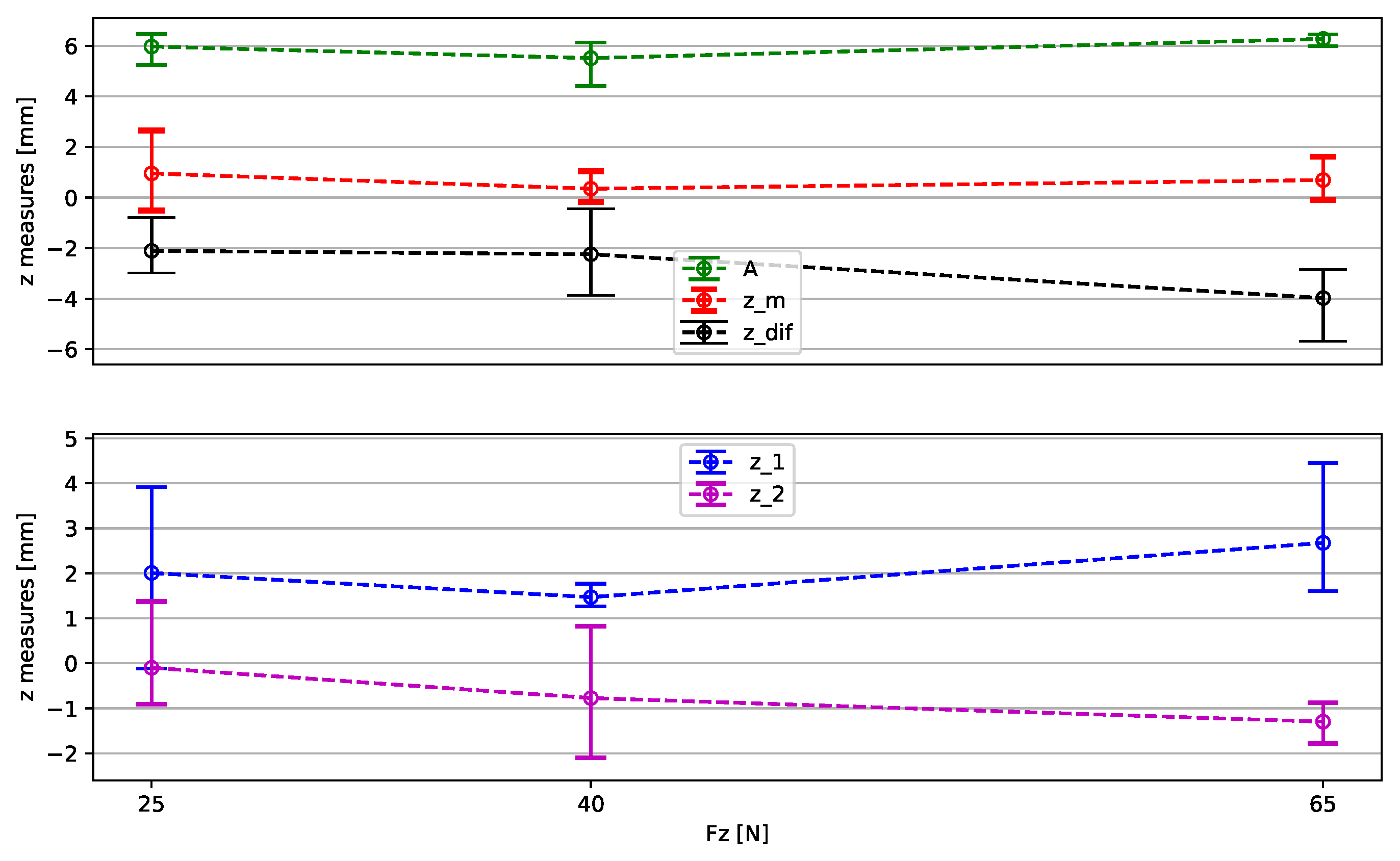
5.2. Discussion About Each Parameter

Regarding the trace length (spatial period T), it virtually did not change among the nine datasets, with an average value of T ¯ = 35.04 mm. The greatest deviation was 0.49% in the dataset 65N1.
The phase, ϕ , is a parameter that was important for correct curve fitting but not for the analysis because it relates to the initial angle at which the wheel was inserted into the sand, and this was not controlled during the experiments. Given that the period is around 34 mm, the phase could assume values from 0 mm to 34 mm, or equivalently, −17 mm to +17 mm.
The amplitude, A, had an average value of A ¯ = 6.09 mm across all the datasets, and the greatest deviation occurred in load case 40N2, being 15.2% smaller than the average. The averages specific to load cases were A ¯ 25 N = 6.242 mm, A ¯ 40 N = 5.766 mm, and A ¯ 65 N = 6.271 mm. We can see that A ¯ 40 N is smaller than the amplitudes for the other two loads. Even if we consider A 40 N 2 an outlier and remove it, the average for the 40 N load case would be A ¯ 40 N = 6.064 mm, which is still smaller than for the other two loads. Overall, the values for amplitude did not have much variation from the mean, and they seem to be unrelated to the amount of vertical load applied. For a visual representation of this, see Figure 18.
Regarding the height at the start, z(290) = z 1 , it had a mean value of z ¯ 1 = 2.07 mm across all the datasets. Separating values for each load case, the mean z 1 height for 25 N was 2.04 mm, and the individual values of z 1 varied, on average, by 1.43 mm from the mean. For 40 N, the mean of z 1 was 1.48 mm, and each individual value varied by only 0.22 mm from that value on average. In the 65 N case, the mean of z 1 was 2.68 mm, and the individual values varied, on average, by 1.18 mm from the mean. Except for the 40 N case, the variation in z 1 values is considered large, and thus, it is difficult to draw a conclusion as to whether it is correlated with the vertical load or not.
For the heights at the end, z(770) = z 2 , the mean across all datasets was −0.72 mm. Looking at each load case, for 25 N, the mean of z 2 was −0.09 mm, and it varied, on average, by 0.97 mm from the mean. The mean of z 2 for the 40 N case was −0.76 mm, and it varied by 1.05 mm on average. For 65 N, the mean of z 2 was −1.30 mm, and it varied, on average, by 0.32 mm from the mean. Overall, the variations in z 2 were large, but considering that the mean values per load decreased consistently (−0.09 mm; −0.76 mm; −1.30 mm) for 25 N, 40 N, and 65 N, respectively, z 2 was arguably correlated with the values of the loads, becoming deeper as the load increased, as can be seen in Figure 18.
One possible value that can be derived from the heights at the start, z 1 , and end, z 2 , is the height at the intermediate position, z m = ( z 1 + z 2 ) / 2 . Looking at the average value of z m for each load, we have 0.97 mm, 0.36 mm, and 0.69 mm, respectively, for loads of 25 N, 40 N, and 65 N. We cannot see a correlation between z m and load. The average values of z m were positive for the three loads, and the overall average across all the datasets was 0.68 mm. For being a positive value, this result shows that, despite the downward force ( F z ) acting on the wheel, the average height of the traces remains above the undisturbed sand level. This phenomenon can be attributed to the observation that during the experiments, the grouser could be seen excavating sand backwards and upwards, which then falls from each grouser, forming the hills that constitute the characteristic wave-shaped traces. Additionally, we hypothesize that the process of lifting and dropping the sand reduces its compaction and bulk density, bringing it into a looser state. This increase in overall volume could explain the higher average height of the traces.
Another value derived from these heights is Δ z = z 2 z 1 . This delta height grouped per load case yields −2.12 mm, −2.24 mm, and −3.97 mm, respectively, for loads of 25 N, 40 N, and 65 N. The continuous increase in the absolute value of Δ z suggests that it grows as the load increases; see Figure 18. This is the same as saying that z 0 ˙ increases with the load, because Δ z is derived from and proportional to z 0 ˙ .

6. Conclusions

This paper reported on the topography of wheel ruts caused by a rover grouser wheel, recorded by LiDAR with SWT apparatus. Three values of vertical force, F z , were used—25, 40 and 65 Newtons—and for each load, the experiment was run three times, resulting in nine datasets. The datasets have been made available to the scientific community through a URL link.
The level of noise in the LiDAR data was considerable; even so, by using a moving average, it was possible to reduce the noise and extract meaningful data by means of curve fitting. A constant horizontal line was used to retrieve the height of the undisturbed sand, and an inclined sine function was used for fitting the ruts caused by the grouser wheel.
A descending trend in the ruts as x increased was present in all nine datasets, and this is believed to have come from the transition from static sinkage to dynamic sinkage. The level of inclination was shown to increase as the vertical load, F z , increased. The trace length did not change across the experiments as it was linked to the slip ratio, which was fixed at 20% in all the test runs. The amplitude was not shown to vary with the load applied as it remained approximately constant across the test runs, with an average value of 6.09 mm.
The average heights of the traces, z m , varied significantly across the test runs. The average value was 0.68 mm, which, being positive, shows that the mean height of the ruts was greater than the original height of the sandbed. It was not possible to find a correlation between the heights z m and F z . The heights of the ruts at the end of the trace, z 2 , had negative values for seven out of the nine test runs, with an average value of −0.72 mm, and these became deeper as the load increased.
Possible applications of this study include calibrating numerical terramechanics simulations like the Discrete Element Method for representing rutting behaviour inside rover simulators such as OmniLRS and for developing vision-based slip detection/ compensation systems.

Future Work

This work used Toyoura sand, so future research should explore a broader range of soils for a more general characterization. In order to further expand this work, other wheel types could be used, with a bigger range of loads, and it would be advantageous to conduct experiments with a rover-mounted sensor in field tests.
The LiDAR sensor used, UST-30LX, in HOKUYO AUTOMATIC CO., LTD, Osaka, Japan presented considerable noise in all scans, making it challenging to extract information in the order of millimeters. Moving averages were used to reduce the level of noise; nevertheless, future studies could try other noise-reduction techniques like Kalman Filtering and the three-sigma rule. More accurate sensors, not based on time-of-flight, could be used to produce a lower level of noise.

Author Contributions

Conceptualization, K.T. and V.E.A.; methodology, K.T. and V.E.A.; software, K.T. and V.E.A.; validation, V.E.A.; formal analysis, V.E.A. and K.T.; investigation, K.T.; resources, K.T. and K.Y.; data curation, K.T.; writing—original draft preparation, V.E.A.; writing—review and editing, K.T., E.R., K.U., and S.S.; visualization, V.E.A., K.T., and E.R.; supervision, K.T., S.S., K.U., and E.R.; project administration, K.T., K.U., and K.Y.; funding acquisition, E.R., K.T., and K.Y. All authors have read and agreed to the published version of the manuscript.

Funding

This research received no external funding.

Data Availability Statement

All data generated or analyzed during this study are included in this published article.

Acknowledgments

The authors would like to thank doctoral student César Bastos da Silva for helping with some data analysis algorithms. This study was financed in part by the Coordenação de Aperfeiçoamento de Pessoal de Nível Superior (CAPES)—Brazil (Finance Code 001), of which author V.E. Ares is a beneficiary. We would like to express our sincere gratitude to Shino Kizaki and Tomomi Tanaka for their assistance in acquiring the experimental data for this study.

Conflicts of Interest

The authors declare no conflicts of interest.

References

  1. McKay, D.S.; Heiken, G.; Basu, A.; Blanford, G.; Simon, S.; Reedy, R.; French, B.M.; Papike, J. The lunar regolith. In Lunar Sourcebook: A User’s Guide to the Moon; Heiken, G.H., Vaniman, D.T., French, B.M., Eds.; Cambridge University Press: Cambridge, UK, 1991; pp. 285–356. [Google Scholar]
  2. Shkuratov, Y.G.; Bondarenko, N.V. Regolith layer thickness mapping of the Moon by radar and optical data. Icarus 2001, 149, 329–338. [Google Scholar] [CrossRef]
  3. Wilcox, B.B.; Robinson, M.S.; Thomas, P.C.; Hawke, B.R. Constraints on the depth and variability of the lunar regolith. Meteorit. Planet. Sci. 2005, 40, 695–710. [Google Scholar] [CrossRef]
  4. Kerr, R.A. Mars Rover Trapped in Sand, But What Can End a Mission? Science 2009, 324, 998. [Google Scholar] [CrossRef]
  5. Wirkus, M.; Hinck, S.; Backe, C.; Babel, J.; Riedel, V.; Reichert, N.; Kolesnikov, A.; Stark, T.; Hilljegerdes, J.; Küçüker, H.D.; et al. Comparative study of soil interaction and driving characteristics of different agricultural and space robots in an agricultural environment. J. Field Robot. 2024, 41, 2009–2042. [Google Scholar] [CrossRef]
  6. Chen, L.; Zou, M.; Chen, Z.; Liu, Y.; Xie, H.; Qi, Y.; He, L. The applications of soil bin test facilities to terramechanics: A review. Rend. Lincei. Sci. Fis. Nat. 2024, 35, 683–703. [Google Scholar] [CrossRef]
  7. Stitch, M.L.; Woodbury, E.J.; Morse, J.H. Optical Ranging System Uses Laser Transmitter. Electronics 1961, 34, 51–53. [Google Scholar]
  8. Saku, Y.; Ishigami, G. Slip Estimation Using Machine Learning of Wheel Trace Patterns for Mobile Robot on Loose Soil. In Proceedings of the 15th European-African Regional Conference of the International Society of Terrain Vehicle Systems (ISTVS), Prague, Czech Republic, 8–11 September 2019. [Google Scholar]
  9. Reina, G.; Ishigami, G.; Nagatani, K.; Yoshida, K. Vision-based estimation of slip angle for mobile robots and planetary rovers. In Proceedings of the 2008 IEEE International Conference on Robotics and Automation, Pasadena, CA, USA, 19–23 May 2008; pp. 486–491. [Google Scholar] [CrossRef]
  10. Gao, H.; Xia, K.; Ding, L.; Deng, Z.; Liu, Z.; Liu, G. Optimized control for longitudinal slip ratio with reduced energy consumption. Acta Astronaut. 2015, 115, 1–17. [Google Scholar] [CrossRef]
  11. Ding, C.; Chang, Y.; Su, Y.; Wang, J.; Xie, M. Rover-Mounted Radar Observation of Discrete Layers Within the Top 4 Meters of Regolith at the Chang’E-3 Landing Site, the Moon. IEEE Trans. Geosci. Remote. Sens. 2024, 62, 1–16. [Google Scholar] [CrossRef]
  12. Allan, M.; Wong, U.Y.; Furlong, P.M.; Rogg, A.; McMichael, S.T.; Welsh, T.M.; Chen, I.; Peters, S.C.; Gerkey, B.P.; Quigley, M.; et al. Planetary Rover Simulation for Lunar Exploration Missions. In Proceedings of the 2019 IEEE Aerospace Conference, Big Sky, MT, USA, 2–9 March 2019; pp. 1–19. [Google Scholar]
  13. Bingham, L.; Kincaid, J.; Weno, B.; Davis, N.; Paddock, E.; Foreman, C. Digital Lunar Exploration Sites Unreal Simulation Tool (DUST). In Proceedings of the 2023 IEEE Aerospace Conference, Big Sky, MT, USA, 4–11 March 2023; pp. 1–12. [Google Scholar] [CrossRef]
  14. Crues, E.Z.; Lawrence, S.J.; Bielski, P.; Jacobs, A.B.; Schlueter, J.; Jagge, A.; Foreman, C.; Raymond, C.; Davis, N. Digital Lunar Exploration Sites (DLES). In Proceedings of the 2022 IEEE Aerospace Conference (AERO), Big Sky, MT, USA, 5–12 March 2022; IEEE: Piscataway, NJ, USA, 2022; pp. 1–13. [Google Scholar]
  15. Kamohara, J.; Ares, V.E.; Hurrell, J.; Takehana, K.; Richard, A.; Santra, S.; Uno, K.; Rohmer, E.; Yoshida, K. Modelling of Terrain Deformation by a Grouser Wheel for Lunar Rover Simulation. In Proceedings of the 21st International and 12th Asia-Pacific Regional Conference of the ISTVS, Yokohama, Japan, 28–31 October 2024. [Google Scholar]
  16. Pieczyński, D.; Ptak, B.; Kraft, M.; Drapikowski, P. LunarSim: Lunar Rover Simulator Focused on High Visual Fidelity and ROS 2 Integration for Advanced Computer Vision Algorithm Development. Appl. Sci. 2023, 13, 12401. [Google Scholar] [CrossRef]
  17. Tasora, A.; Serban, R.; Mazhar, H.; Pazouki, A.; Melanz, D.; Fleischmann, J.; Taylor, M.; Sugiyama, H.; Negrut, D. Chrono: An open source multi-physics dynamics engine. In Proceedings of the High Performance Computing in Science and Engineering: Second International Conference, HPCSE 2015, Soláň, Czech Republic, 25–28 May 2015; Revised Selected Papers 2. Springer: Berlin/Heidelberg, Germany, 2016; pp. 19–49. [Google Scholar] [CrossRef]
  18. Higa, S.; Nagaoka, K.; Yoshida, K. Reaction force/torque sensing wheel system for in-situ monitoring on loose soil. In Proceedings of the 19th International and 14th European-African Regional Conference of the International Society for Terrain-Vehicle Systems (ISTVS), Budapest, Hungary, 25–27 September 2017. [Google Scholar]
  19. Takehana, K.; Kizaki, S.; Uno, K.; Tanaka, T.; Suda, G.; Yoshida, K. Evaluation and Comparison of Driving Performance of Lunar Exploration Rover Wheel in Different Soils. In Proceedings of the 16th European-African Regional Conference of the ISTVS, Lublin, Poland, 11–13 October 2023. [Google Scholar]
  20. Ozaki, S.; Ishigami, G.; Otsuki, M.; Miyamoto, H.; Wada, K.; Watanabe, Y.; Nishino, T.; Kojima, H.; Soda, K.; Nakao, Y.; et al. Granular flow experiment using artificial gravity generator at International Space Station. NPJ Microgravity 2023, 9, 61. [Google Scholar] [CrossRef] [PubMed]
  21. Mitchell, J.; Houston, W.; Carrier III, W.; Costes, N. Apollo Soil Mechanics Experiment S-200; Final Report. Technical Report 15, Issue 7; Space Sciences Laboratory: Berkeley, CA, USA, 1974; NASA Contract NAS 9–11266. [Google Scholar]
  22. Fa, W. Bulk Density of the Lunar Regolith at the Chang’E-3 Landing Site as Estimated From Lunar Penetrating Radar. Earth Space Sci. 2020, 7, e2019EA000801. [Google Scholar] [CrossRef]
  23. Almaeeni, S.; Els, S.; Almarzooqi, H. To a Dusty Moon: Rashid’s Mission to Observe Lunar Surface Processes Close-Up. In Proceedings of the 52nd Lunar and Planetary Science Conference, The Woodlands, TX, USA, 15–19 March 2021; p. 1906. Available online: https://www.hou.usra.edu/meetings/lpsc2021/pdf/1906.pdf (accessed on 19 September 2024).
Figure 1. SWT with Rashid Rover wheel installed and resulting ruts.
Aerospace 12 00071 g001
Figure 2. Single-wheel testbed from Space Robotics Lab, Tohoku University [19].
Aerospace 12 00071 g002
Figure 3. Model of wheel of Rashid rover used to create the ruts [19].
Aerospace 12 00071 g003
Figure 4. Experiment to determine LiDAR accuracy.
Aerospace 12 00071 g004
Figure 5. Plot from LiDAR accuracy experiment with heights extracted.
Aerospace 12 00071 g005
Figure 6. Different values of moving average applied to LiDAR data.
Aerospace 12 00071 g006
Figure 7. Moving average (z_ma) with 15 data points applied to 9 datasets.
Aerospace 12 00071 g007
Figure 8. Definition of heights and incline used in this paper.
Aerospace 12 00071 g008
Figure 9. Average bed height in black and curve fit of sine wave in red. Dataset 25N1.
Aerospace 12 00071 g009
Figure 10. Average bed height in black and curve fit of sine wave in red. Dataset 25N2.
Aerospace 12 00071 g010
Figure 11. Average of bed height in black and curve fit of sine wave in red. Dataset 25N3.
Aerospace 12 00071 g011
Figure 12. Average of bed height in black and curve fit of sine wave in red. Dataset 40N1.
Aerospace 12 00071 g012
Figure 13. Average bed height in black and curve fit of sine wave in red. Dataset 40N2.
Aerospace 12 00071 g013
Figure 14. Average bed height in black and curve fit of sine wave in red. Dataset 40N3.
Aerospace 12 00071 g014
Figure 15. Average bed height in black and curve fit of sine wave in red. Dataset 65N1.
Aerospace 12 00071 g015
Figure 16. Average bed height in black and curve fit of sine wave in red. Dataset 65N2.
Aerospace 12 00071 g016
Figure 17. Average bed height in black and curve fit of sine wave in red. Dataset 65N3.
Aerospace 12 00071 g017
Figure 18. Relevant parameters extracted: amplitude A, z_1, z_2, z_m, and z_dif ( Δ z ). The points represent the average value per load case, and the error bars are used to show the lowest and highest values found in each test run.
Aerospace 12 00071 g018
Table 1. Comparison of mechanical properties of Toyoura sand and regolith simulant and measurements from Apollo and Chang’E-3 missions.
QuantityToyoura Sand [20]Regolith Simulant (<425 μm) [20]Lunar Samples [21]
Particle size 50% (μm)26213942–128
Particle size max (μm)675675-
Bulk density (g/cm3)1.378–1.6311.497–1.9080.85–2.25 [22]
Particle density (g/cm3)2.6612.899-
Angle of repose (deg)36.0--
Friction angle (deg)31.0–40.433.9–46.735–1.5
Cohesion (kPa)0.6–2.80.3–3.20.03–2.1
Table 2. Relative heights of box objects.
ObjectLeft Height
(mm)
Deviation
(mm)
Right Height
(mm)
Deviation
(mm)
Big, sand27.37−2.6330.960.96
Small, sand6.80−3.209.75−0.25
Big, green26.32−3.6828.98−1.02
Small, green6.71−3.295.84−4.16
Big, white30.250.2528.88−1.12
Small, white0.18−9.821.00−11.00
Table 3. Bed heights and MSE error metric of horizontal line fit.
SampleBed Height
(mm)
Mean Square
Error (mm)
25N 1−369.042.43
25N 2−370.191.45
25N 3−368.634.60
40N 1−366.511.85
40N 2−370.541.40
40N 3−366.361.44
65N 1−373.261.02
65N 2−372.744.97
65N 3−372.451.45
Table 4. Lower and upper bounds of parameters for sine fit.
Intercept z 0 Incline z 0 ˙ Amplitude APhase ϕ Period T
Lower bound−380−0.012205.1−1.534.86
Upper bound−355−0.000936.53435.18
Table 5. Parameters extracted from sine fit ( z 0 : intercept; z 0 ˙ : incline; A: amplitude; ϕ : phase; T: period).
Sample z 0 (mm) z 0 ˙ (mm/mm)A (mm) ϕ (mm)T (mm)
25N 1−368.67−0.001696.45821.3635.03
25N 2−364.64−0.005516.272−1.4734.95
25N 3−364.52−0.006365.9988.3335.13
40N 1−364.97−0.000946.12428.0035.13
40N 2−366.34−0.008245.1708.7835.16
40N 3−363.49−0.005136.00533.3635.17
65N 1−369.57−0.007206.37230.8434.88
65N 2−369.01−0.006076.45230.8634.96
65N 3−364.49−0.012105.99120.7035.02
Table 6. Sine fit error metrics.
SampleMean Square
Error (mm)
Mean
Error (mm)
Maximum
Error (mm)
25N 12.861.404.16
25N 22.201.204.38
25N 32.141.164.91
40N 11.641.043.63
40N 23.321.535.02
40N 32.651.304.72
65N 11.811.123.41
65N 21.601.043.61
65N 31.901.094.67
Table 7. Sine fit with relative height—A: amplitude; ϕ : phase; T: period; z 1 : z at beginning of wave; z 2 :z at end of wave.
SampleA (mm) ϕ (mm)T (mm) z 1 (mm) z 2 (mm)
25N 16.45821.3635.03−0.11−0.91
25N 26.272−1.4734.953.951.36
25N 35.9988.3335.132.27−0.72
40N 16.12428.0035.131.260.82
40N 25.1708.7835.161.81−2.06
40N 36.00533.3635.171.38−1.04
65N 16.37230.8434.881.60−1.78
65N 26.45230.8634.961.97−0.88
65N 35.99120.7035.024.45−1.23
Disclaimer/Publisher’s Note: The statements, opinions and data contained in all publications are solely those of the individual author(s) and contributor(s) and not of MDPI and/or the editor(s). MDPI and/or the editor(s) disclaim responsibility for any injury to people or property resulting from any ideas, methods, instructions or products referred to in the content.

