Abstract
The complexity and resource-sharing nature of traffic within multi-airport regions present significant challenges for air traffic management. This paper aims to develop a mesoscopic traffic model for exploring the traffic dynamics under coupled operations, and thus to conduct capacity decoupling analysis. We propose an integrated surface–airspace model. In the surface model, we utilize linear regression and random forest regression to model unimpeded taxiing time and taxiway network delays due to sparsity of ground traffic. In the airspace model, a dualized queuing network topology is constructed including a runway system, where the fluid queuing model is applied, and an inter-node traffic flow transmission mechanism is introduced to simulate airspace network traffic. Based on the hybrid and efficient model, we employ a Monte Carlo approach and use a quantile regression envelope model for capacity decoupling analysis. Using the Shanghai multi-airport region as a case study, the model’s performance is validated from the perspectives of operation time and traffic throughput. The results show that our model accurately represents traffic dynamics and estimates delays within an acceptable margin of error. The capacity decoupling analysis effectively captures the interdependence in traffic flow caused by resource sharing, both within a single airport and between airports.
1. Introduction
With the context of global economic advancement, the civil aviation industry has become a significant driver of economic growth. The convenience and efficiency of air transportation have provided people worldwide with more accessible travel options and generated substantial economic and social benefits. However, the rapidly growing demand for air transport has further highlighted issues such as flight delays and capacity–demand imbalances. As the primary focus of air traffic management systems, the terminal maneuvering areas (TMA) are particularly susceptible to congestion, delays, and safety hazards due to the intricate nature of their internal traffic flows [1]. Although some intervention measures have been implemented at busy airports to mitigate congestion and address capacity–demand imbalances, these issues remain difficult to resolve fully [2]. Meanwhile, regional economic development has expanded TMA boundaries, leading to multiple airports sharing airspace resources. Although resource sharing offers potential to mitigate air traffic congestion, the operational coupling between airports during peak periods may intensify resource competition, necessitating dynamic capacity allocation across airports [3]. Capacity, as one of the key parameters in air traffic management (ATM), directly shapes the operational efficiency of the air traffic. Therefore, it is necessary to conduct a capacity decoupling analysis and accurately determine capacity parameters for coupled multi-airport regions.
The complex interrelationships between airports make capacity evaluation in multi-airport regions significantly more challenging than for a single airport. This demands the systematic incorporation of resource allocation dynamics and operational constraints—such as ground procedures, weather, and air traffic control (ATC) procedures [4,5,6]—into capacity evaluation frameworks for multi-airport systems. Existing methods for assessing and determining airport capacity can generally be classified into three main categories: (a) mathematical modeling approaches, (b) data analysis approaches and (c) traffic flow modeling approaches. In the early stage, research primarily focused on mathematical modeling approaches. In 1959, Blumstein first introduced a theoretical airport capacity model, establishing a series of mathematical expressions to estimate aircraft separation intervals and, consequently, airport capacity [7]. Subsequent studies further refined mathematical methods in areas such as traffic flow composition and aircraft combination [8,9,10]. However, due to the inherent simplicity of mathematical formulations, these models struggled to capture the stochastic characteristics of operations. Capacity assessment methods based on empirical analysis and historical data aim to establish the interdependence between departure and arrival traffic, typically represented as a convex capacity curve. The concept of capacity envelopes was first introduced by Gilbo in 1993 [11]. Subsequently, methods such as quantile regression, scenario-based optimization, and chance-constrained optimization were applied to estimate the airport capacity envelope [3,12,13]. While such data-driven methods effectively capture historical operational characteristics, they remain limited in their ability to explore the upper bounds of capacity.
Another approach is traffic flow modeling, which can be broadly categorized into microscopic, mesoscopic, and macroscopic based on levels of fidelity. Microscopic models, including commercial tools such as SIMMOD and TAAM, simulate individual aircraft trajectories with high fidelity by considering detailed airport layouts [14]. However, their primary limitations include high modeling costs and significant computational demands. Macroscopic traffic models study the relationships between flow, density, and speed, along with aggregation variables. These models typically focus on global traffic information rather than merely local traffic states. Some common macroscopic models include the Modified Menon Model (MMM), Cell Transmission Model–Large Capacity (CTM-L), the 2D Eulerian Flow Model and the Linear Dynamic Systems Model (LDSM) [15,16,17,18]. Despite their lower fidelity, macroscopic models show the advantage of fast simulation due to their simplicity. Mesoscopic traffic models link system elements, often integrating queuing theory to capture traffic dynamics. However, many studies rely on the assumptions of known distribution, limiting their applicability. Research suggests that a general distribution-based queuing theory approach does not depend on Poisson or exponential distribution assumptions, providing more realistic terminal area traffic flow modeling [19,20]. Mesoscopic models balance simulation fidelity with computational efficiency, addressing microscopic models’ high cost and complexity. However, they often require extensive data for accurate implementation.
In summary, considerable research has been conducted on methods and models for airport capacity assessment. However, most of these approaches are confined to single airports and seldom consider multi-airport regions, especially in terms of the integration of air and ground traffic. Furthermore, with respect to evaluation results, many studies offer a fixed capacity value. In the context of coupled and resource-sharing multi-airport regions, such capacity parameters fail to accurately capture the interdependence between airports. In this paper, we propose an integrated surface–airspace traffic model to perform capacity decoupling analysis for multi-airports. The main contributions of this paper can be summarized as follows:
- We developed a hybrid and integrated surface–airspace traffic model, combining linear regression, the random forest algorithm and fluid queuing theory. Focusing on the Shanghai multi-airport region, the validity and accuracy of the proposed traffic model in capturing the coupled traffic dynamics are shown with empirical data;
- Using the Monte Carlo simulation approach, we take the integrated traffic model as a platform, and propose a frequency-constrained envelope quantile regression model. This model is used to analyze the interdependence among various traffic flows within the coupled multi-airport region, ultimately obtaining dynamic capacities in the form of envelope curves.
The structure of this paper is organized as follows. Section 2 describes the framework of the integrated traffic model and the modeling of both airport surface traffic and terminal airspace traffic. Airport surface taxiing time is decomposed into unimpeded taxiing time and taxiway network delay, while TMA airspace is represented as a queuing network topology based on Instrument Flight Procedures (IFPs). This section also introduces the fluid queuing model and the transmission mechanism between nodes. Section 3 details the generation of random samples based on the traffic model, and presents the quantile regression-based envelope model with frequency constraints. Section 4 provides a case study of the Shanghai multi-airport system, detailing model parameter calibration, the validation of the hybrid-integrated traffic model, and the decoupling analysis of traffic flow dependencies across intra-airport and inter-airport operational scenarios. Finally, Section 5 presents the summary and outlines directions for future research.
2. Integrated Modeling of Surface–Airspace Traffic for Multi-Airport Coupled Operation
2.1. Framework of the Integrated Traffic Model
Spatially, aircraft operations can be divided into airport surface taxiing and TMA airspace flying. Accordingly, this study establishes two dedicated models—the surface traffic model and the TMA airspace traffic model—to capture these operational dynamics. Building on our previous research [21], we can decompose the airport surface taxiing time into three components: unimpeded taxiing time, taxiway network delay, and runway queue waiting time. A hybrid model combining linear regression, the random forest algorithm and queuing theory will be used to predict these three components.
The proposed airspace traffic model conceptualizes TMA resources as discrete queuing system nodes, forming a queuing network, and uses fluid queuing theory to simulate the traffic dynamic. It is important to note that to ensure consistency in the modeling approach, the runway, as a critical link between the surface model and the airspace model, will be modeled as part of the airspace model.
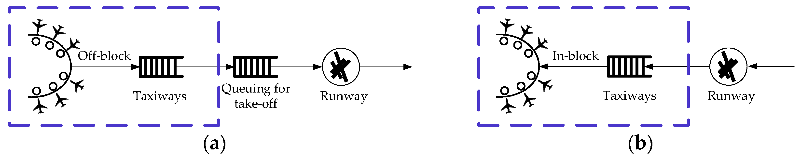
As shown in Figure 1, for departing flights, the traffic flow enters the surface traffic model based on the off-block time, which outputs the time to reach the runway entry point. After determining the runway waiting time, the takeoff time is derived and input into the airspace model. Finally, the flight exits the TMA at the departure fix. For arriving flights, the traffic flow simulation starts at the arrival fix. The traffic flow based on the arrival fix time is input into the airspace model, which outputs airborne delays and land-on-time. Then, we input the traffic flow into the surface model to determine unimpeded taxiing time and taxiway network delays, ultimately providing the in-block time. It should be noted that the runway waiting time for arriving flights is not represented in the surface model, but occurs within the airspace model.
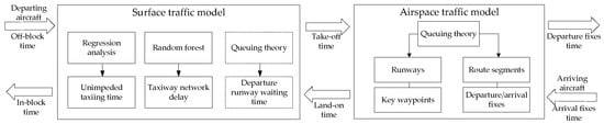
Figure 1.
The framework of the integrated surface–airspace traffic model.
2.2. A Hybrid Model for Airport Surface Operation
In departure and arrival operations, the dominant mode of surface operations manifests as aircraft taxiing. The taxiing time is a crucial metric for evaluating the efficiency of aircraft taxiing on the airport surface. The taxi-out process can be divided into two stages for departing flights, as depicted in Figure 2a. The first stage involves the aircraft taxiing from the gate to the runway entry point, and the second stage is the waiting-for-take-off period at the runway entry point. For arriving flights, the surface taxiing time does not encompass the waiting time on the runway. As shown in Figure 2b, it is solely manifested in the stage when the aircraft taxis from the touchdown point to the gate.

Figure 2.
A schematic of the aircraft operation process. (a) For departure traffic; (b) for arrival traffic.
In this subsection, the airport surface taxiing modeling is centered around two specific stages: the taxiing of departing flights from the gate to the runway entry point and the taxiing of arriving flights from the touchdown point to the gate. These are the sections within the blue dashed boxes in Figure 2. This modeling consists of two components: the unimpeded taxiing time and the taxiway network delay.
2.2.1. Unimpeded Taxiing Time
The unimpeded taxiing time is the nominal operational time between the gate and the runway under optimal operating conditions [22]. It does not include any taxiing pauses or waiting times caused by potential operational conflicts, traffic control, etc. During the taxiing process, due to factors such as taxiing routes, taxiing speeds, and runways, the unimpeded taxiing time may fluctuate to some extent. The impact of differences in taxiing routes and distances is more prominent for large airports. The unimpeded taxiing time is usually calculated according to its gate and runway. However, specific gate assignments are not available in the strategic flight schedule. This study calculates the unimpeded taxiing time based on apron sectorization [23], and the unimpeded taxiing time is calculated according to different apron areas and runways. Therefore, this study calculates the unimpeded taxiing time based on apron sectorization [23], considering variations across distinct apron zones and their corresponding runway configurations.
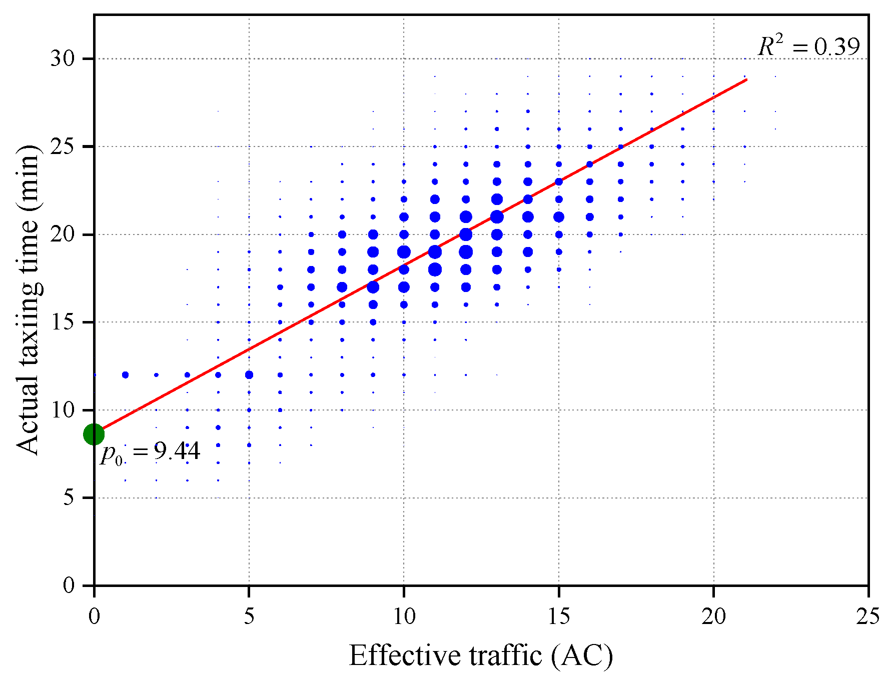
An effective surface traffic value is used as the independent variable, and linear regression is adopted to fit the taxiing time [24]. For the taxi-out process, this index is defined as the sum of the number of aircraft taxiing out on the surface when the flight pushes back and the number of aircraft pushing back during the taxi-out period. Similarly, for arriving flights, this value is equal to the sum of the number of aircraft taxiing in on the surface when the aircraft lands and the number of aircraft landing during the taxi-in period. Based on historical operation data, the correlation between the surface traffic index and the taxiing time is established. The calculation is shown in Equation (1) and an example is given in Figure 3.

Figure 3.
The regression for the unimpeded taxi-in time from No. 8 apron to runway 34R at Shanghai Pudong Airport.
2.2.2. Taxiway Network Delay
Aircraft are vulnerable to various uncertain factors during the taxiing process. When taxiing conflicts or congestion occur, aircraft usually must stop and wait, resulting in delays in taxiing. Due to the complexity and sparsity of aircraft flow operations in the taxiway network, it is difficult to estimate the taxiway network delay using analytical models directly. This section adopts a data-driven approach based on the aircraft surface taxiing situation indices. The specific steps and ideas are as follows:
- 1.
- Extract the actual taxiway network delay
Firstly, based on the historical operation data of complex airports, we extract fundamental information about aircraft, including flight numbers, aircraft types, airlines, parking stands, and runways. Additionally, we obtain the time points of crucial operational events such as off-block, take-off, landing, and in-block. Subsequently, we assign the unimpeded taxiing time for each aircraft.
The actual taxiing time for departing aircraft consists of three components: the unimpeded taxiing time, taxiway network delay, and runway queuing time. Since the runway queuing time cannot be directly obtained from the existing data, we approximate the runway queuing time using the fluid queuing model described in Section 2.3.2. Thus, the taxiway network delay for departing flights is determined by subtracting the unimpeded taxiing time and runway queuing delay from the actual taxiing time. Considering the distinction in the taxiing process for arriving aircraft, the taxiway network delay is equal to the difference between the actual taxiing time and the unimpeded taxiing time.
- 2.
- Calculate the aircraft surface taxiing index at the airport
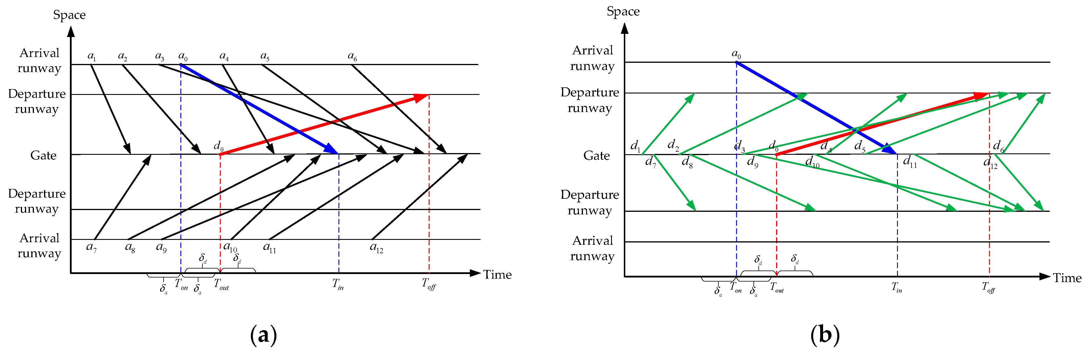
The features in the training set are calculated based on the Macroscopic Distribution Network (MDN) of the taxiing process at the airport [25]. As shown in Figure 4, from a macroscopic perspective, we can build 16 features according to the spatiotemporal distribution of aircraft under different taxiing situations. In the figure, (denoted by the blue line) and (denoted by the red line) are the arriving reference aircraft and the departing reference aircraft, respectively. It should be noted that not all time points used in the calculations are derived from historical data. We approximate the take-off and landing time using Equations (2) and (3). This approach avoids the paradox of training a real-delay prediction model with known take-off or landing time, as accurate take-off and landing times are unavailable in delay prediction research based on strategic flight plans.
where , , and are the approximate landing time, actual in-block time, actual off-block time, and approximate take-off time, respectively.

Figure 4.
Spatiotemporal Macroscopic Distribution Network diagram. (a) Diagram of arrivals; (b) diagram of departures.
In Figure 4a, black lines represent other arriving aircraft on the airport surface, whereas green lines in Figure 4b represent other departing aircraft. Based on the different circumstances of the reference aircraft, the features for taxiway network delay are established, and their definitions are displayed in Table 1. The table presents four primary categories of features: Surface Instantaneous Flow Indices (SIFIs), Surface Cumulative Flow Indices (SCFIs), Aircraft Queue Length Indices (AQLIs), and Slot Resource Demand Indices (SRDIs). Each category comprises four distinct features. The prefixes D and A denote that the calculation pertains to departing and arriving aircraft, respectively, while the prefix R signifies that the calculation scenario involves the same or same-side runway.

Table 1.
Definition and calculation examples of the surface taxiing index.
- 3.
- Train a Random Forest Model
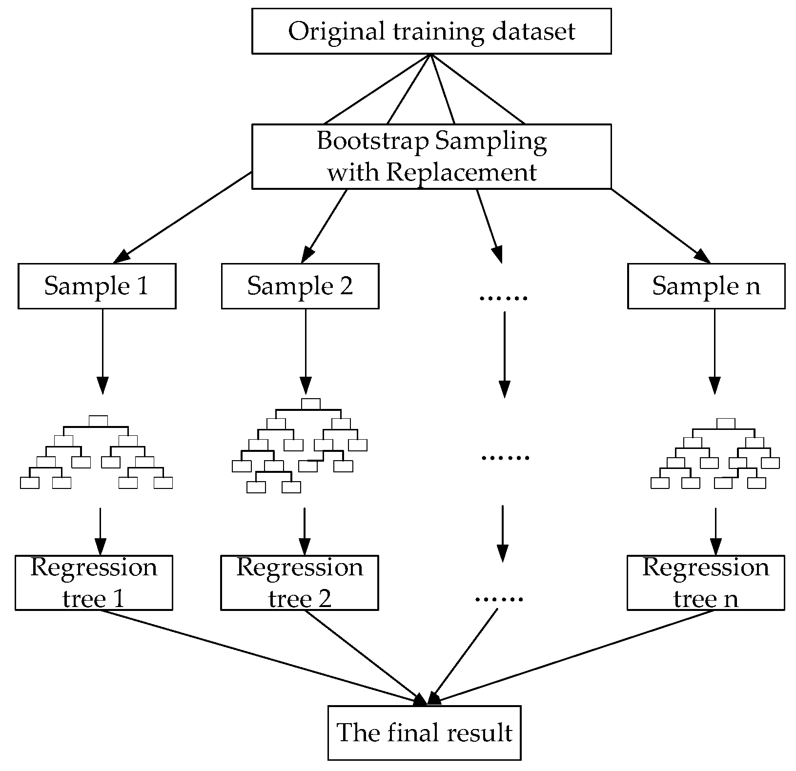
We construct a training dataset using these indices as features and the taxiway network delays as the target variable. We then apply the random forest algorithm for machine learning modeling, a method widely utilized for predicting taxiing time and delays [26]. Random forest is an ensemble learning technique based on decision trees, which creates multiple decision trees by randomly selecting different data samples from the same training set. This approach effectively reduces variance at the expense of a slight increase in bias and a reduction in interpretability. For regression problems, the final prediction is determined by the mean of the predictions from multiple trees, as illustrated in Figure 5. By calculating the surface taxiing indices for each aircraft and inputting them into the trained model, we can obtain the taxiway network delay for each aircraft.

Figure 5.
The diagram of the random forest algorithm.
2.3. Queuing Network Model for Terminal Airspace
The airspace structure of multi-airport TMA is highly complex, with strong and intricate operational coupling between airports. This complexity presents significant challenges for modeling and capacity evaluation. This study focuses on the physical topology of the multi-airport terminal area, emphasizing the operational dynamics of key resources such as runways, air route segments, and departure/arrival fixes. From a mesoscopic modeling perspective, we propose a fluid queuing network model for the terminal airspace. Given the modeling complexity and real-world traffic conditions, the following assumptions are made:
- Assumption 1. The model neglects the interrelationship between the arrival and departure IFPs. Although they share common waypoints, air traffic control regulations typically separate the crossing points by altitude to minimize their mutual impact;
- Assumption 2. Aircraft flying through the terminal airspace are assumed to have independent flight times on their segments, following a specific service time distribution. Airborne delays arise from the waiting time generated when the system exceeds its service capacity upon the aircraft entering into the queueing system;
- Assumption 3. Once an aircraft enters the terminal airspace, it will follow the Standard Instrument Flight Procedures (SIFPs). Even in scenarios involving sustained queueing due to resource constraints, aircraft maintain adherence to their assigned nodes without altering their predefined flight paths or operational procedures;
- Assumption 4. For generality, the model does not consider hazard weather, military activities, or temporary traffic control measures.
2.3.1. Dualized Queuing Topology Network
In the complex multi-airport TMA, runways, air routes, and departure/arrival fixes function as independent queuing systems serving as “servers,” while aircraft act as “customers”. IFPs consist of spatial flight paths formed by a series of waypoints and route segments, interwoven within the airspace to create a complex network structure. We define this point–edge network as the Standard Route Network (SRN), which serves as the foundation for the TMA airspace queuing topology. In the SRN, the vertices record the latitude and longitude coordinates of the waypoints, while the edges record the start and end waypoints of the route segments.
Traversing a route segment takes time, whereas passing through a waypoint occurs instantaneously, which differs from the expected queuing nodes. This discrepancy motivates our proposed dual-network transformation of the SRN, where the route segments replace the vertices to explicitly model the temporally distributed nature of segment traversal. According to the spatial connectivity among the approach and departure air route segments, they can be classified into five types: unit segment, continuous segments, diverging segments, converging segments, and intersecting segments. The corresponding dualization criteria for each type of segment are as follows:
- Unit segment. A basic segment between two waypoints, representing the smallest component of an IFP. In dualization, a unit segment corresponds to a single node, as shown in Figure 6;

Figure 6.
The dualization of the unit segment.
Figure 6.
The dualization of the unit segment.

- Continuous segments. As illustrated in Figure 7, a continuous segment consists of multiple unit segments. After dualization, it forms a sequential arrangement of nodes and edges;

Figure 7.
The dualization of the continuous segments.
Figure 7.
The dualization of the continuous segments.

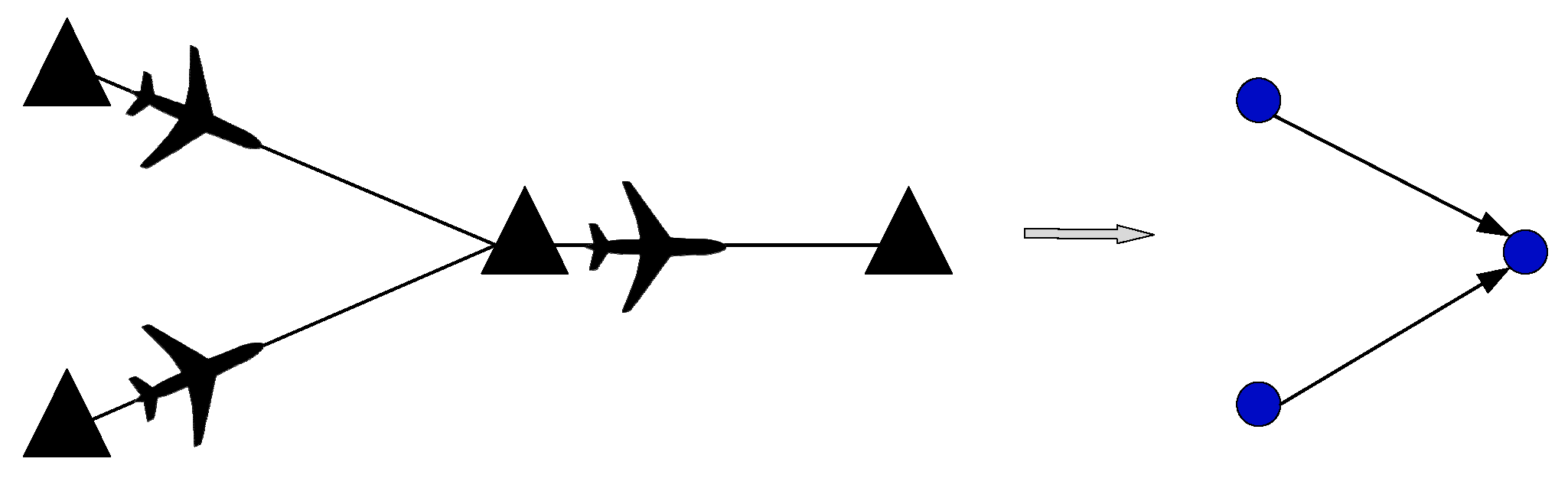
- Converging segments. As illustrated in Figure 8, converging segments occur when two or more segments with different directions pass through the same waypoint and subsequently merge into a single segment with a unified direction;

Figure 8.
The dualization of the converging segments.
Figure 8.
The dualization of the converging segments.
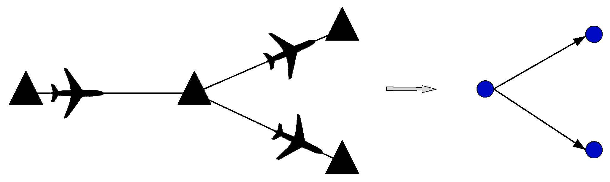
- Diverging segments. Diverging segments occur when an aircraft transitions into two or more segments with different directions after passing through a waypoint. This is common in departure turns or multi-airport TMA where arriving aircraft are directed to different airports. The dualization of diverging segments is shown in Figure 9;
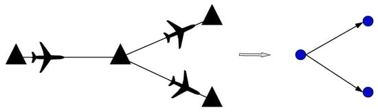
Figure 9.
The dualization of the diverging segments.
Figure 9.
The dualization of the diverging segments.
- Intersecting segments. Intersecting segments involve two or more segments with different directions converging at a shared waypoint and subsequently diverging into separate segments.
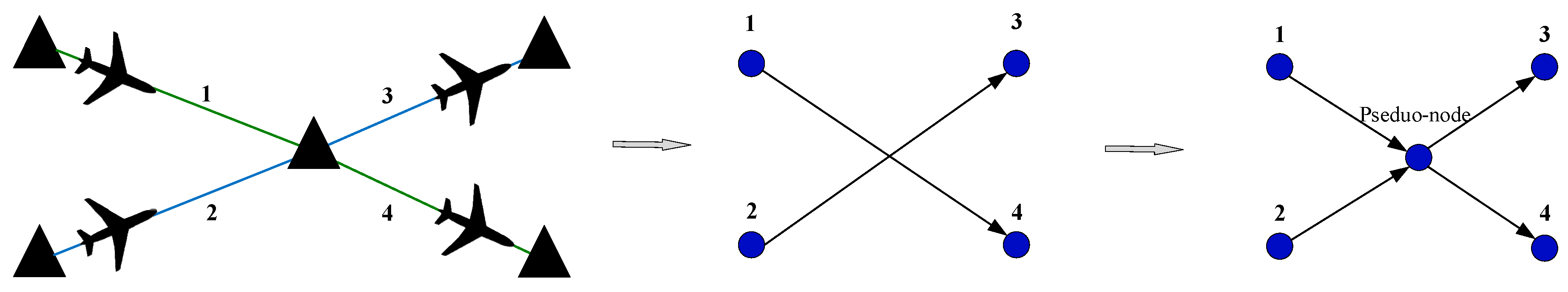
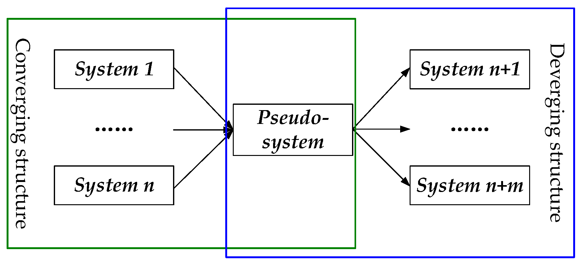
As shown in Figure 10, such waypoints act as critical resource-sharing hubs for convergence and divergence, and are referred to as key waypoints. Aircraft passing through these waypoints must strictly adhere to specific separation requirements to ensure operational safety and stability. Consequently, queuing and delays at these waypoints are often unavoidable.

Figure 10.
The dualization of the intersecting segments.
The conventional “edge–node” dualization approach is inadequate for accurately capturing the resource-sharing dynamics at key waypoints. To address this issue, this study introduces pseudo nodes to model these key waypoints with “many-to-many” connectivity, as shown in Figure 10. It should be noted that aircraft in Segment 1 cannot be transferred to Segment 3, as the two segments are not connected in the original SRN. The same applies to Segment 2 and Segment 4.
In the queuing network model for multi-airport TMA, other key resources include runways and departure/arrival fixes. These elements constitute the primary interface nodes governing traffic initiation and termination within TMA operations, and require particular attention. Accordingly, this study also adopts pseudo nodes to abstract runways and departure/arrival fixes, extending the network model outward.
Thus, we obtain the dualized SRN, the topology network in the multi-airport terminal airspace. Under this framework, arriving aircraft operations begin at a pseudo arrival fix server. After entering the TMA, aircraft transition to the segment servers connecting arrival fixes to subsequent waypoints. After completing a series of segment operations within the TMA, aircraft flow through the final approach segment server, await runway service, and proceed to surface taxiing. The operation of departing aircraft commences with surface taxiing, followed by queuing at the departure runway server for takeoff. Aircraft transition into the airspace, fly towards the departure fix and reach the pseudo-departure fix server.
2.3.2. Fluid Queue Model for a Single Node
In the dualized SRN, each node represents a queuing system. To ensure the model’s applicability, in this paper, a G(t)/GI/s(t) time-varying fluid queuing model is employed to simulate each queuing system. This model consists of a time-varying general arrival process and a general independent service process with a time-varying service capacity. The arrival process is characterized by a time-varying arrival rate. The service time refers to the flight time of an aircraft as it traverses through this system, which satisfies the assumption of independent and identical distribution. The service capacity is the maximum number of aircraft that can be served simultaneously in the service system.
In the fluid queuing model, the traffic flow is approximated as a continuous fluid, and the aircraft is assumed to be infinitely divisible objects, similar to the flow of fluid rather than discrete entities. One of its key advantages is handling non-stationary queuing models. In this paper, the deterministic fluid model proposed by Whitt [27] with the First-Come First-Served (FCFS) principle is applied to approximate the stochastic queuing process of the traffic flow at a single service node in the network.
Firstly, we denote the quantity of flow that enters the queue system over the time interval , which is equal to the integral of the arrival rate over this time period.
We have the probability density function for service time. We define the cumulative distribution function , the complementary cumulative distribution function and the hazard function , as follows.
Next, we focus on two key performance descriptors, and . Specifically, represents the quantity of aircraft in service at time that have been in service for a time no more greater , while represents the number of aircraft in queue at time that have been waiting for a time less than or equal to .
where and represent the fluid densities of aircraft in service and in the queue, respectively, which are non-negative and integrable.
Thus, we can obtain and , which represent the total quantity of aircraft in service and the total quantity of aircraft waiting in queuing at time t. From the above, we know that the initial values of and are determined by and . In this case, five key functions, λ(t), s(t), G, b(0,y), and q(0,y), determine a G(t)/GI/s(t) queue model.
In this model, there are two conditions of flow—the under-load (UL) condition and the over-load (OL) condition.
When (1) or (2) , , and , the UL condition starts at time . We define the time when the UL condition terminates and then switch to the OL condition as in Equation (10).
where the quantity of aircraft in service and the quantity of aircraft that complete service are defined via Equations (11) and (12). In Equation (12), is calculated as in Equation (13).
Similarly, when (1) or (2) , , , the OL condition starts at time . The time when the OL condition terminates is defined as in Equation (14).
where the quantity of aircraft waiting in the queue and in Equation (X) are given by Equations (15) and (16).
Generally, we pay much attention to the waiting time during the OL period, which is denoted as . In Equation (17), represents the quantity of aircraft entering the service.
Therefore, we can approximate the total waiting time over a period, given by Equation (19).
where represents the number of OL periods during the simulation time during the ith OL period, is the mean of waiting time, and is the quantity of aircraft entering the system.
2.3.3. Inter-Node Traffic Flow Transmission Mechanisms
We introduced the queuing simulation of a single-server system earlier. In the complex terminal area SRN, queuing systems formed by key resource nodes facilitate traffic flow connectivity through intricate interactions. This study proposes a dynamic simulation framework based on the fluid queuing network to accurately capture traffic flow dynamics in multi-airport terminal areas.
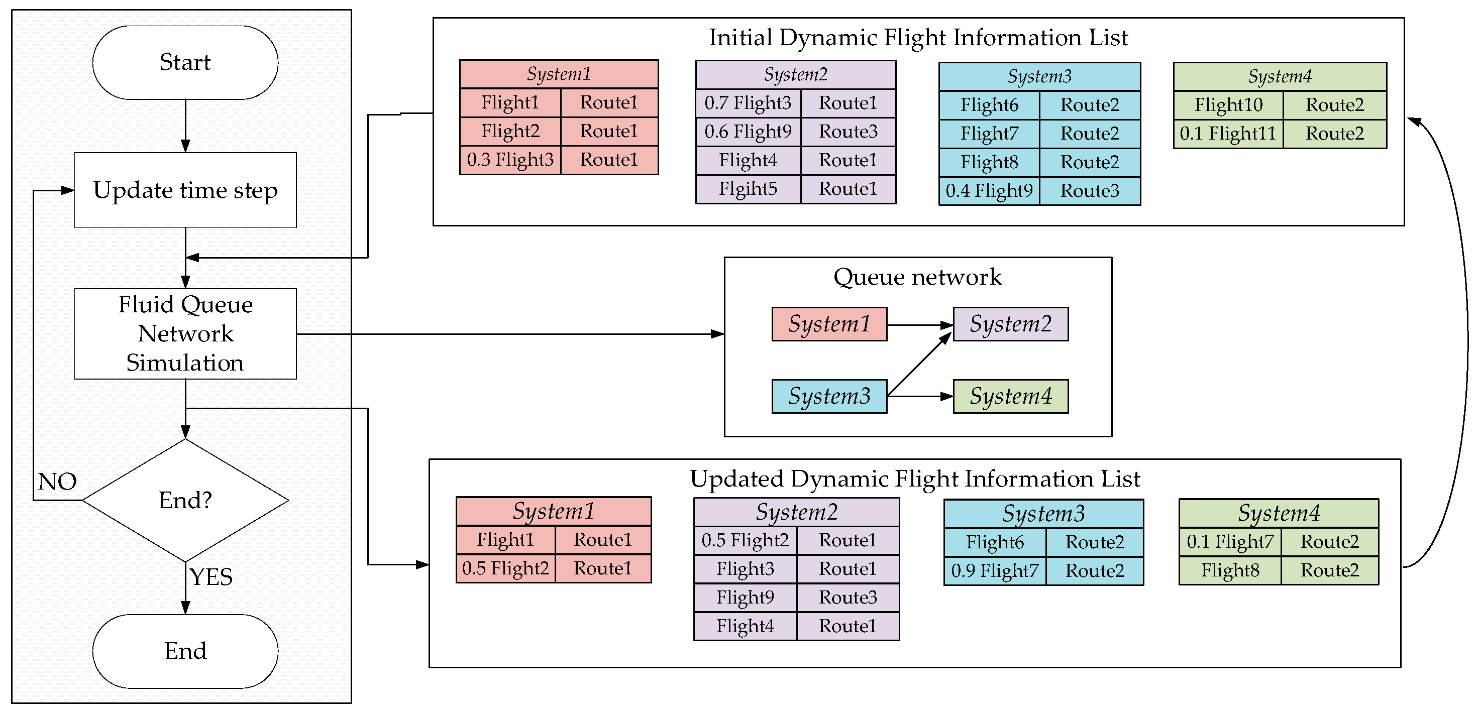
To reduce computational costs and enhance result clarity, a fixed time-step approach is used to update and monitor the states of nodes within the queuing network. To ensure precise flight tracking and monitoring, the simulation is based on the First-In-First-Out (FIFO) assumption, and a dynamic flight information list is designed to store the relevant data for each node. This list records the current key resource point, callsigns, and predefined flight paths in the queue. The overall dynamic simulation framework of the fluid queuing network is shown in Figure 11. Based on this framework, the delay time of each flight can be estimated, which is the sum of the waiting times encountered at all the service nodes it passes through.
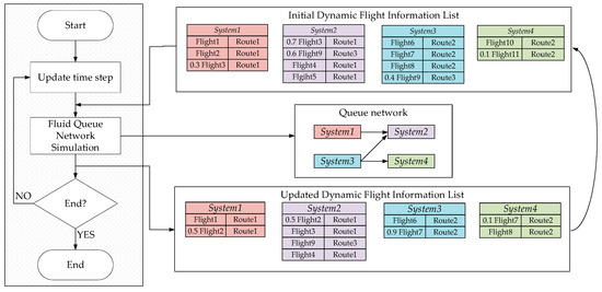
Figure 11.
Dynamic simulation framework for the fluid queuing network model.
Next, we will explain the simulation and transmission mechanisms of traffic under various connectivity structures in the queuing network.
- Tandem structure
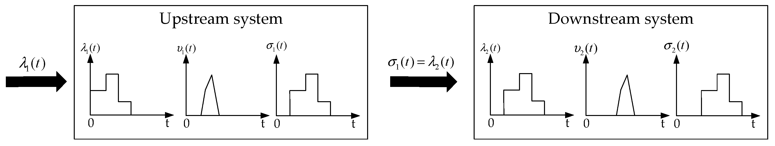
Figure 12 illustrates the most common connectivity in a queuing network, where a single upstream node is connected to a downstream node. Aircraft pass through the upstream queuing system and then immediately enter the downstream system following the First-In-First-Out (FIFO) principle. This implies that the departure rate of the upstream queuing system is equal to the arrival rate of the downstream system, which means .

Figure 12.
Traffic transmission under the tandem structure.
- 2.
- Diverging Structure
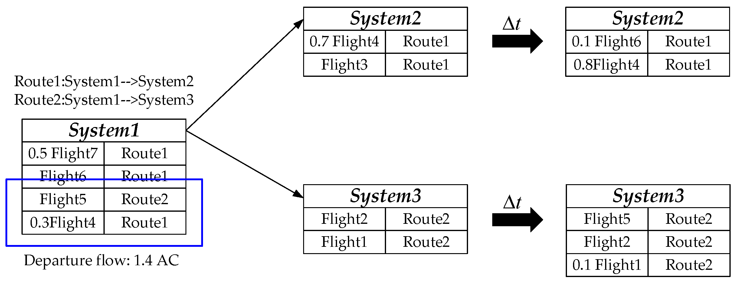
A diverging structure refers to a case wherein a single upstream node connects to multiple downstream nodes, commonly observed at points such as the departure runway, the connection to the TMA, and between diverging route segments. As shown in Figure 13, we can calculate the number of aircraft departing from the upstream queuing system at each update step. The proportion of traffic flow directed downstream is determined by the flight routes of the departing aircraft. The arrival for each downstream node is then updated according to the scheduled flight routes and the FIFO principle.

Figure 13.
Traffic transmission under the diverging structure.
- 3.
- Converging Structure
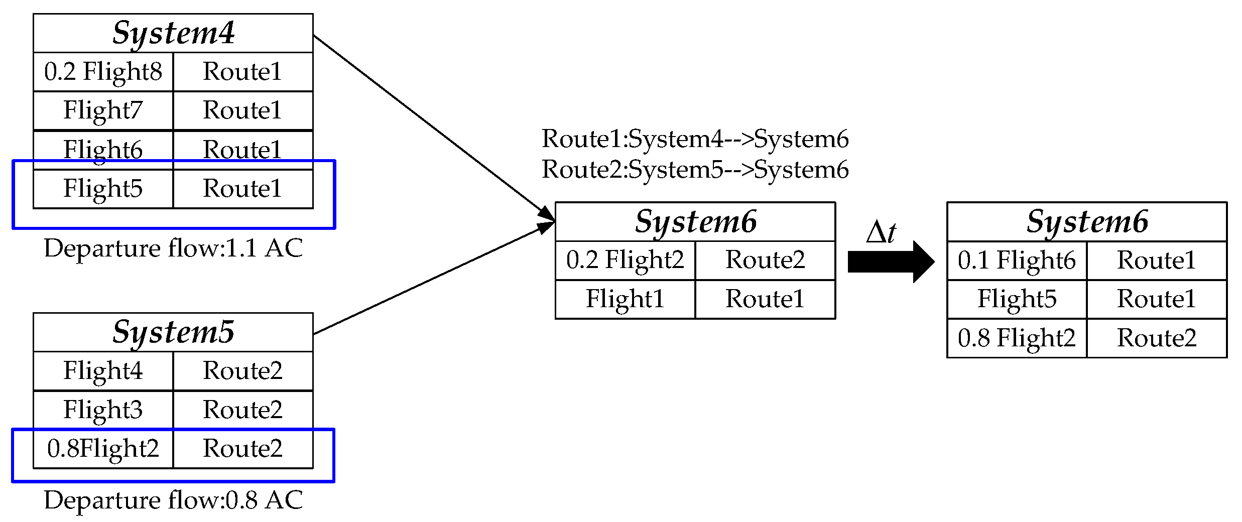
A converging structure refers to a case wherein multiple upstream nodes converge to a single downstream node, as shown in the Figure 14. This structure is commonly observed in the TMA, such as in the case of five-airport flights converging to the arrival runway and between converging route segments. The arrival rate of the downstream queuing system is the sum of the departure rates from all upstream systems, i.e., . There is no priority order among the traffic flow from upstream nodes; instead, the traffic flows are randomly transferred to the downstream system in sequence.
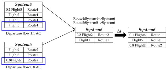
Figure 14.
Traffic transmission under the converging structure.
- 4.
- Intersecting Structure
In Section 2.2.1, we used pseudo-nodes to dualize the intersecting segments. This intersecting queuing structure can be divided into a converging structure and a diverging structure, as shown in Figure 15. Following the transmission rules for traffic flow in both the diverging and converging structures, the flow first converges from multiple upstream nodes into the pseudo-queuing system, and then diverges from the pseudo-queuing system to the downstream nodes.
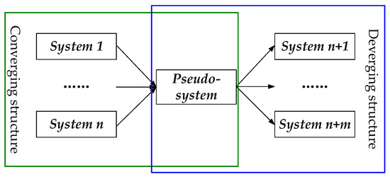
Figure 15.
Traffic transmission under the intersecting structure.
3. Capacity Decoupling Based on Envelope Modeling
Airport capacity is a key parameter for flight schedule configuration. Currently, capacity evaluation for multi-airport systems, mainly based on technologies such as commercial simulation software, can determine a fixed capacity value for the entire system and each airport. However, such a fixed and unique capacity parameter fails to reflect the dynamic interactions between airports, and cannot adequately balance the relationship between airport operational efficiency and demand. We intend to adopt a Monte Carlo simulation approach, generating a large number of flight schedules randomly, and input them into the traffic model we built above to obtain the expected delay time. A frequency-constrained envelope quantile regression model is proposed to decouple the capacity of the multi-airport regions based on the sample data.
3.1. Generating Random Samples
The Monte Carlo method simulates and predicts complex system behavior through random sampling, approximating solutions via numerous random trials. Its key steps include defining problem parameters and their probability distributions, generating random samples, conducting simulations, and analyzing results. Within this framework, we propose to conduct a flight augmentation experiment based on historical flight schedule data. The primary advantage of using historical flight data as the sampling source is that they not only provide detailed records of key flight information, such as callsign, aircraft type, gate, runway, and IFP, but they also capture the operational rules of the airport and the historical distribution of the flights. Additionally, SIFPs for each flight are assigned according to the historical frequency distribution of city pairs, ensuring that the random allocation accurately reflects real-world patterns. Based on the integrated surface–airspace model, we can estimate expected delays for any input flight schedule. Thus, we obtain quantities of samples, which serve as the foundational data for the coupling capacity evaluation of the multi-airport regions in the next section.
3.2. Capacity Analysis Through Envelope Modeling
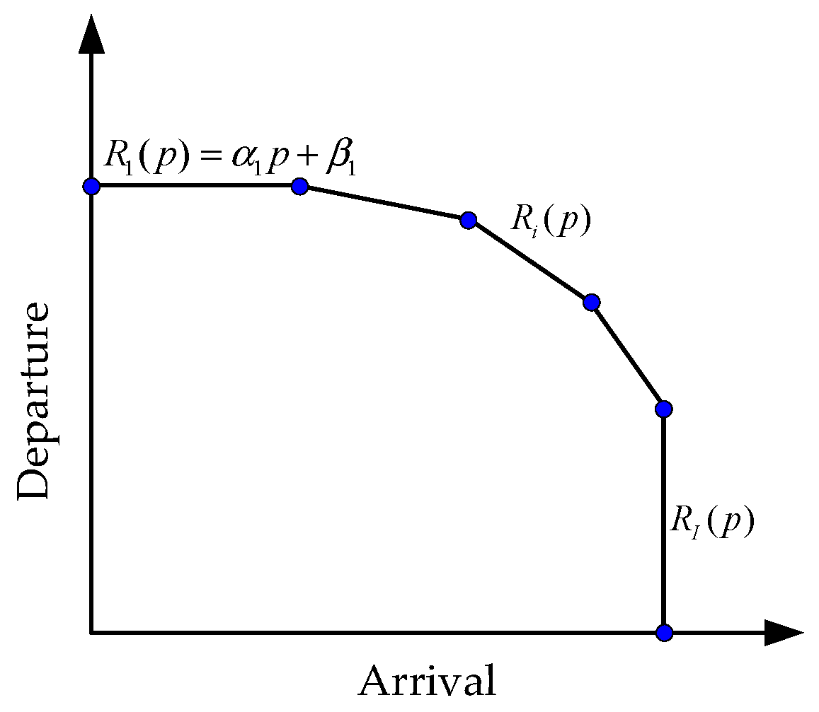
This study adopts the envelope modeling approach to capture the complex interrelationships within the coupled multi-airport regions. An envelope is a convex capacity curve that reflects the interdependent relationship between traffic flows using a convex and nonlinear function, shown in Figure 16. This method was first introduced by Newell in 1979 to analyze the relationship between arrival and departure flows [28]. In 1993, Gilbo, using historical operational data, proposed an airport capacity envelope model based on data frequencies [11]. Building upon existing methods, this paper introduces a frequency-constrained envelope quantile regression model, which builds piecewise linear convex functions to elucidate the coupled interdependence between arrival and departure traffic flows.

Figure 16.
An example of envelope curves.
We consider a two-dimensional dataset of air traffic sample as , i.e., . These data points can represent either the arrival and departure traffic flows within the same airport during the same time period, or any combination of arrival and departure traffic flows across multiple airports within a regional multi-airport system during the same time period.
Let the envelope be represented by a piecewise linear function, as in Equation (20).
where , and represent the slope and intercept of the k-th segment of the piecewise linear function, respectively.
Based on the properties of quantile regression and convex functions, we have developed a linear optimization model to predict the slope and intercept of each segment function at the -th quantile.
In Equation (22), constraints (1) and (2) represent the non-increasing and convex properties of the envelope function, respectively. Constraint (3) ensures the continuity of the envelope. In constraint (4), D(⋅) denotes the delay function of the integrated surface–airspace model. The valid samples in the envelope model must satisfy a certain delay threshold requirement.
4. Case Study
4.1. Data Description
This paper presents a case study focusing on two airports in Shanghai, China—Shanghai Hongqiao International Airport (ICAO code: ZSSS) and Shanghai Pudong International Airport (ICAO code: ZSPD). The Shanghai multi-airport region serves as a typical example, with both airports sharing common departure/arrival fixes and air routes, resulting in significant interactions between their internal traffic flows. The following section provides a detailed overview of the surface layout and operational regulations, the structure of the terminal airspace, and the historical data. All data processing, model construction, and computational implementation in this study were executed using Python 3.10.
- Surface layout and operational regulations
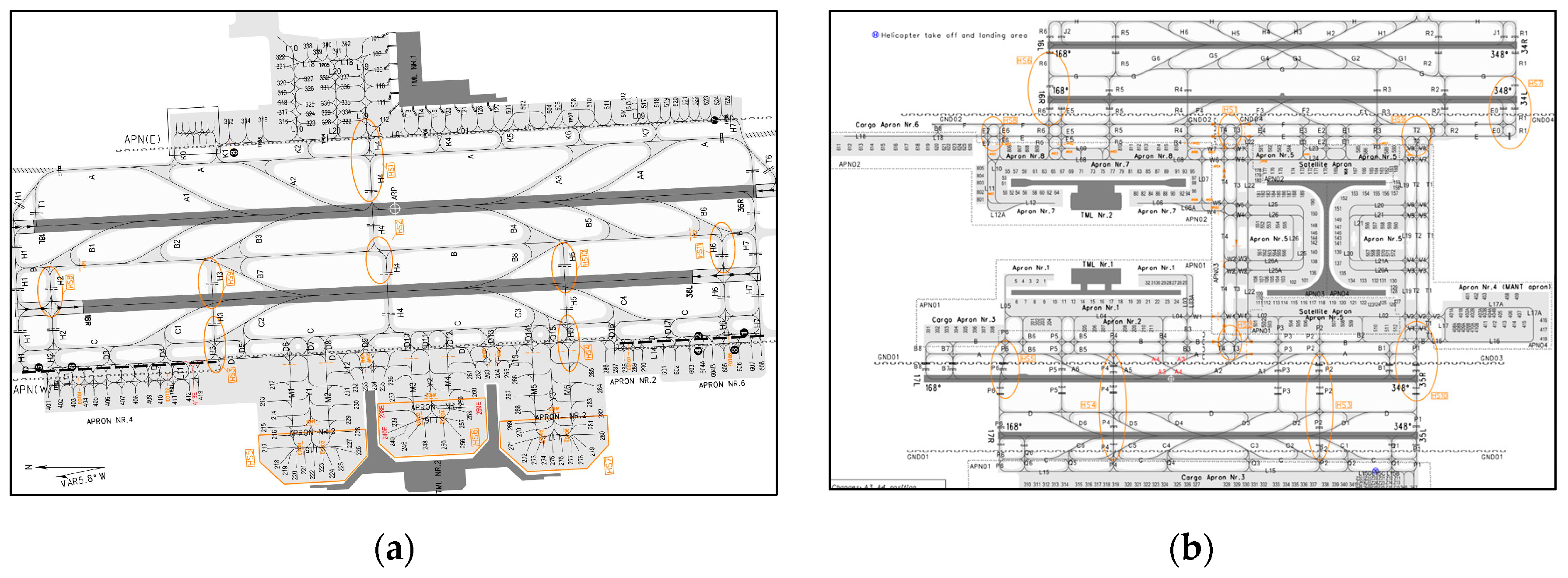
A summary of the surface layout is provided in Figure 17. ZSSS has two runways, 18L/36R and 18R/36L, and 138 gates. It operates in a parallel independent mode, with the eastern runway, 18L/36R, designated for landing and the western runway, 18R/36L, for take-off. ZSPD currently operates four runways, 17R/35L, 17L/35R, 16R/34L, and 16L/34R, along with 340 gates. Among these, 17L/35R and 16R/34L are primarily used for take-off, while 17R/35L and 16L/34R are mainly designated for landing.

Figure 17.
Surface layout and structure. (a) ZSSS; (b) ZSPD.
- 2.
- Structure of the terminal airspace
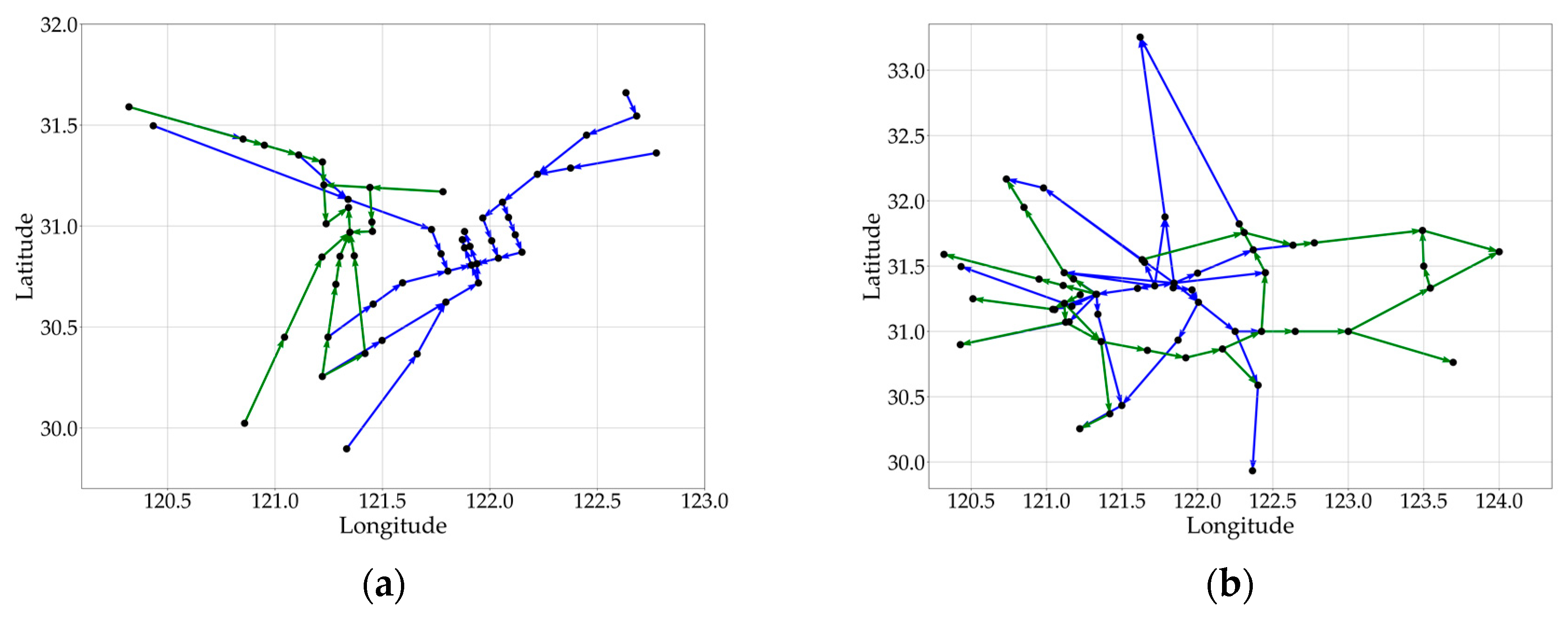
For ZSSS, arrival flights primarily enter from PIKAS, NXD, PINOT, and SASAN, while departure flights mainly leave from PIKAS, NXD, AND, and BONGI. For ZSPD, arrival flights mainly enter from BK, AND, SASAN, DUMET, and MATNU, while departure flights mainly leave from AND, HSN (PONAB), MIGOL, LAMEN, SURAK, NXD, SASAN, ODULO (IBEGI), and PIKAS. The SRN formed by SIFPs under northbound operations in the Shanghai terminal area is shown in Figure 18, where green lines and blue lines denote SIFPs from ZSSS and ZSPD, respectively.

Figure 18.
The SRN under northbound operations in the Shanghai terminal area. (a) Arrival SIFPs; (b) departure SIFPs.
- 3.
- Historical data
The historical data used in this study primarily consist of historical operational data and historical radar flight trajectory data from 2019. The historical flight operation data mainly record information such as flight callsign, departure and landing airport, gate, runway, scheduled and actual off/in block time, as well as actual takeoff and landing time. The historical radar flight trajectory data provide a detailed record of the flight trajectories, and are a time series for the same aircraft, with timestamps and geographical information. In this study, the radar trajectory data for 2019 have a sampling interval of 4 s, with each sample recording the instantaneous latitude, longitude, altitude, and horizontal speed of each aircraft.
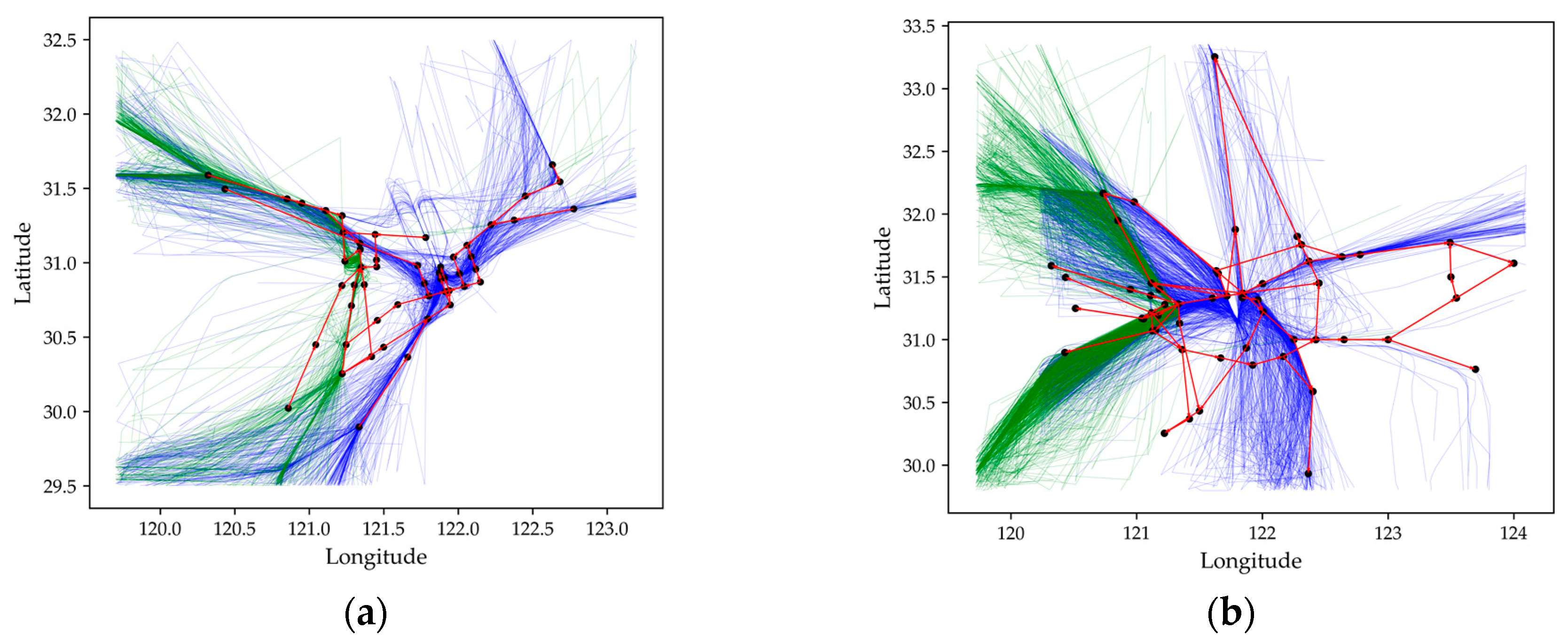
As shown in Figure 19, we mapped historical radar trajectory data onto the SRN in red [29]. The trajectories in green represent flights from ZSSS, while the trajectories in blue correspond to flights from ZSPD. Through mapping, we can establish the spatiotemporal correspondence between the trajectories and the real network, allowing us to extract flight operation information.

Figure 19.
The mapping relationship between historical trajectories and SRN: (a) arrival traffic; (b) departure traffic.
4.2. Model Parameters
- 1.
- Unimpeded taxi time
The unimpeded taxi time is a key parameter in the “surface” model, determined by establishing a linear relationship between the actual taxiing time of flights and the effective surface traffic values. The actual taxi-out time is calculated as the difference between the actual takeoff time and the off-block time, while the actual taxi-in time is the difference between the in-block time and the landing time. To ensure the reliability of the experimental data, outlier taxiing times are removed using the 3σ-rule.
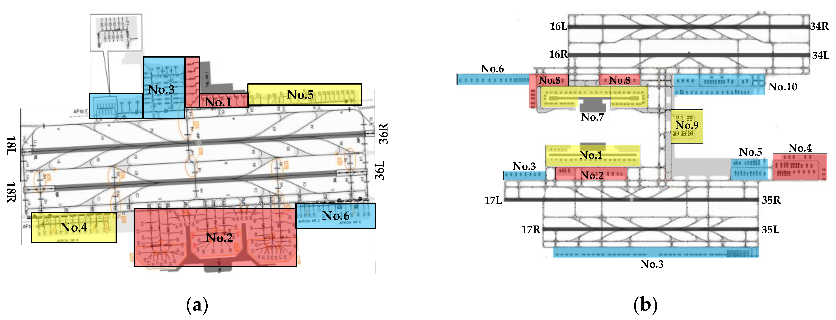
Based on sectorization, the apron at ZSSS is divided into six sections, while the apron at ZSPD is divided into ten sections. The layout of these sections is shown in Figure 20. The results for unimpeded taxiing time are presented in Table 2 and Table 3.

Figure 20.
The sectorization of the apron area. (a) ZSSS; (b) ZSPD.
Table 2.
The unimpeded taxiing time at ZSSS.
Table 3.
The unimpeded taxiing time at ZSPD.
- 2.
- Arrival rate
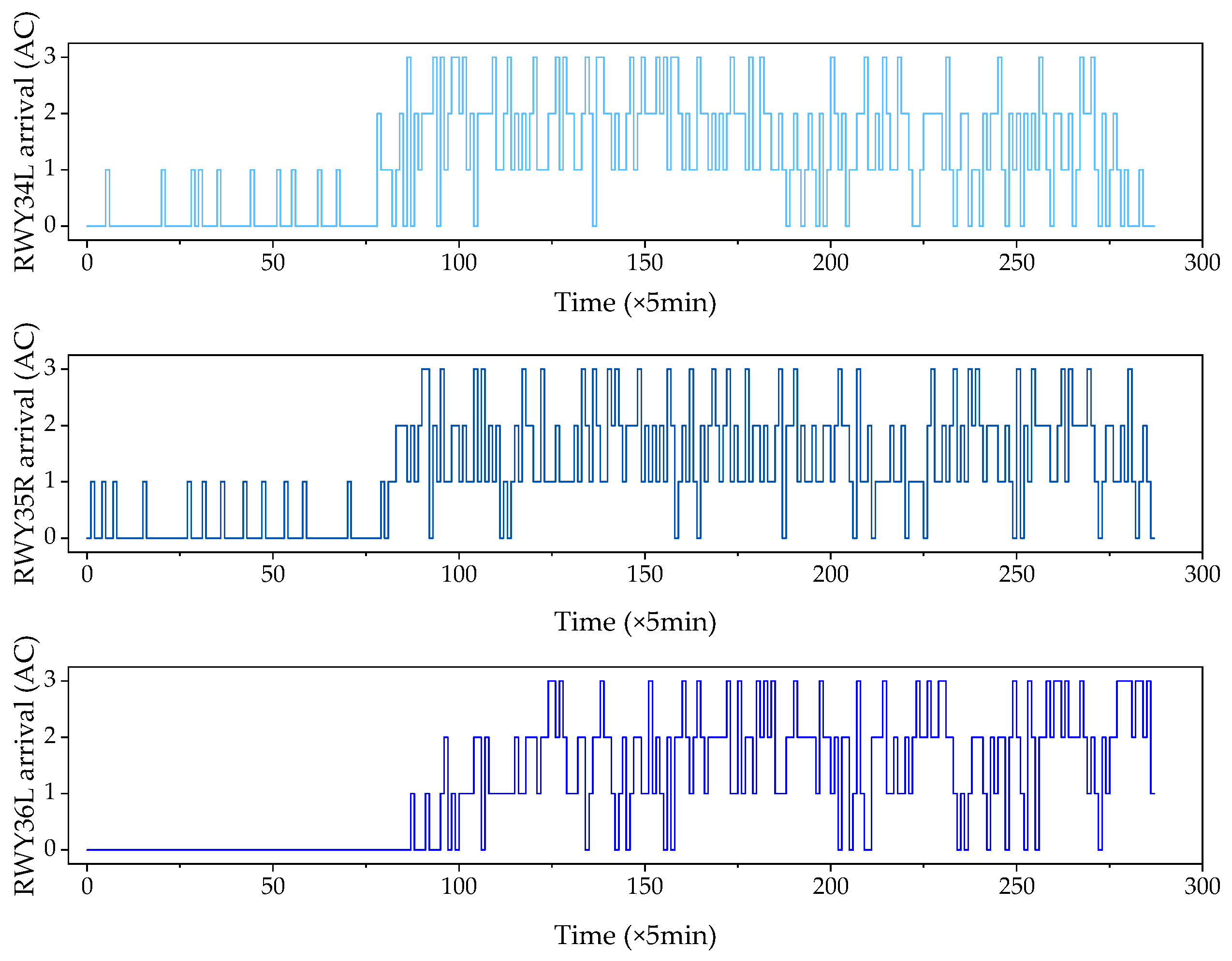
When validating the airspace traffic model using historical operational data from a typical day, the actual times at the arrival fixes are known and directly serve as the input for the arrival airspace queue network model. The flight sequence from the departure surface model is used as the input traffic flow for the departure airspace model. In this case study, the arrival rate is grouped over a specific time interval, denoted as , where represents the number of aircraft arriving at the queuing node within the time range . If the time interval is too large, it will fail to capture the time-varying characteristics of the input traffic flow. Conversely, if the time interval is too small, it will lead to excessive data, increasing the computational burden and complexity of data processing. Referring to the study by Itoh [20], a time interval of 5 min is set in this study to calculate the arrival rate. The arrival distribution at the arrival fixes is shown in Figure 21, and the arrival rate distribution of departing aircraft on each departure runway is shown in Figure 22.
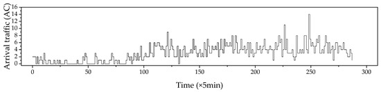
Figure 21.
The arrival distribution at the arrival fixes.

Figure 22.
The arrival distribution on each departure runway.
- 3.
- Service time
The queuing network consists of three service nodes: runways, route segments, and pseudo queue nodes. The service time for a route segment is defined as the time difference between passing two waypoints. The historical distribution of flight times for a segment is used as the service time distribution.
Runway service time refers to the sum of runway occupancy time and wake separation time. However, accurately extracting these two times from historical data can be challenging. In this study, we set the runway service time to 2 min, based on the minimum separation time required between consecutively landing or departing aircraft under ideal operational conditions.
For pseudo queue nodes formed by key waypoints and departure/arrival fixes, the service time distribution is controlled within a fixed monitoring time step to ensure that it does not significantly affect the overall flight time. In this study, the monitoring time step is set to 20 s. The historical maximum crossing speed is denoted as , and the pseudo distance of the node is calculated as multiplied by the monitoring time step. The service time distribution for the pseudo queue system is then derived by dividing the pseudo distance by the historical speed distribution.
- 4.
- Service capacity
In the airspace queuing network model, each system has a specific service capacity limit, representing the maximum number of aircraft the system can accommodate and service at a given time. When an aircraft arrives at a queue system, if there is remaining capacity, the aircraft is allowed to enter the system and receive the service. Conversely, the aircraft will join the waiting queue if the node has reached its service capacity and there is no available space. Meanwhile, the waiting room is assumed to be infinite.
For the case study, each system has a fixed service capacity. The runway queue has a service capacity of 1, that is ; for route segment in TMA, the service capacity is determined by dividing the segment distance by the air traffic control separation interval. The control separation interval in the Shanghai terminal area is set to 10 km. For the pseudo queue system, the service capacity is calculated based on the pseudo distance, with different separation intervals applied. The control separation interval for key intermediate waypoints is 10 km, the terminal transfer interval for departure is 30 km, and the terminal transfer interval for arrival is 20 km.
4.3. Validation of the Integrated Traffic Model
A typical day was randomly selected to validate the integrated surface–airspace traffic model in the Shanghai terminal areas. Based on the calibration of the key parameters mentioned earlier, this section assesses the model’s accuracy from two perspectives: operational time and traffic throughput.
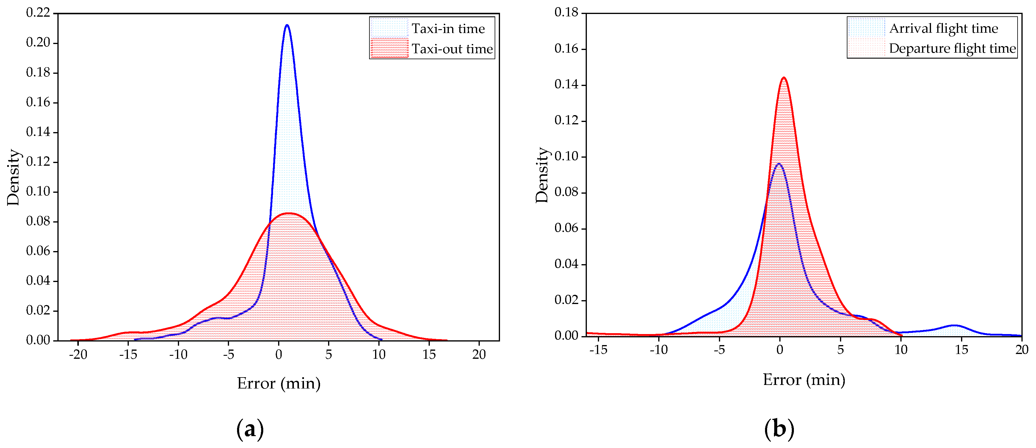
Aircraft operations within the airport terminal area are generally divided into two phases: taxiing on the surface and flying in the airspace. We input a typical flight schedule into the simulation model and extracted each aircraft’s predicted taxiing and terminal flight times for comparison with actual values. Figure 23 presents the error density distribution of predicted versus actual times for both inbound and outbound flights. The errors are predominantly clustered around zero, with the majority of error density peaks skewed above zero, suggesting that the model tends to overestimate operational time. This overestimation is due to the model’s strict adherence to runway intervals and separation requirements during simulation. In practice, however, controller maneuvers can help mitigate delays.
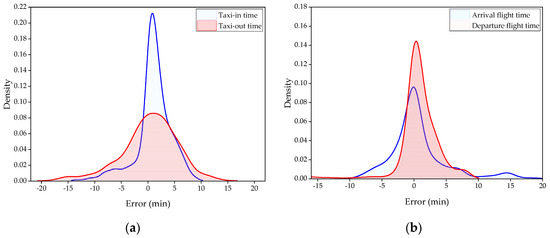
Figure 23.
Density distribution of prediction errors in operation time. (a) Taxiing times; (b) flight times.
The primary operational time point for inbound flights is the aircraft’s touchdown on the runway. In this model, the simulation of inbound flight flows begins at the arrival fixes, meaning that the error in airspace flight time is equivalent to the prediction error in landing times. As shown in Table 4, the mean error (ME) for landing times is 0.65 min, with a mean absolute error (MAE) of 2.82 min. Similarly, for outbound flights, the key operational time point is the aircraft’s departure from the runway, with taxiing time error directly reflecting the takeoff time prediction error. The data in Table 4 indicate that the mean prediction error for taxiing-out time is 0.32 min, with an MAE of 3.57 min. These results demonstrate that the model is capable of predicting key operational time points for both inbound and outbound flights within an acceptable margin of error. Additionally, Table 4 presents prediction errors for inbound taxiing times and outbound flight times, both of which show low mean prediction errors, highlighting the model’s high simulation accuracy.
Table 4.
The average prediction error in operation time.
It is important to note that, in order to ensure consistency in the statistical comparison between actual and predicted takeoff times, the predicted pushback times incorporate delays due to the departure runway queue system. This inclusion is made despite the fact that runway queue modeling is not integrated into the airport surface taxiing prediction framework in this study.
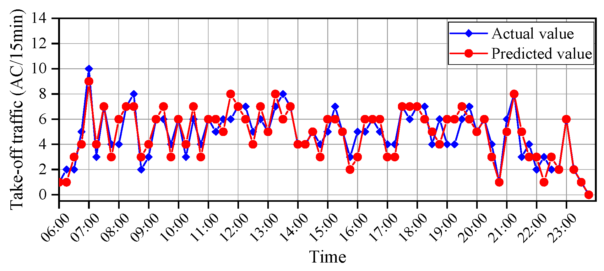
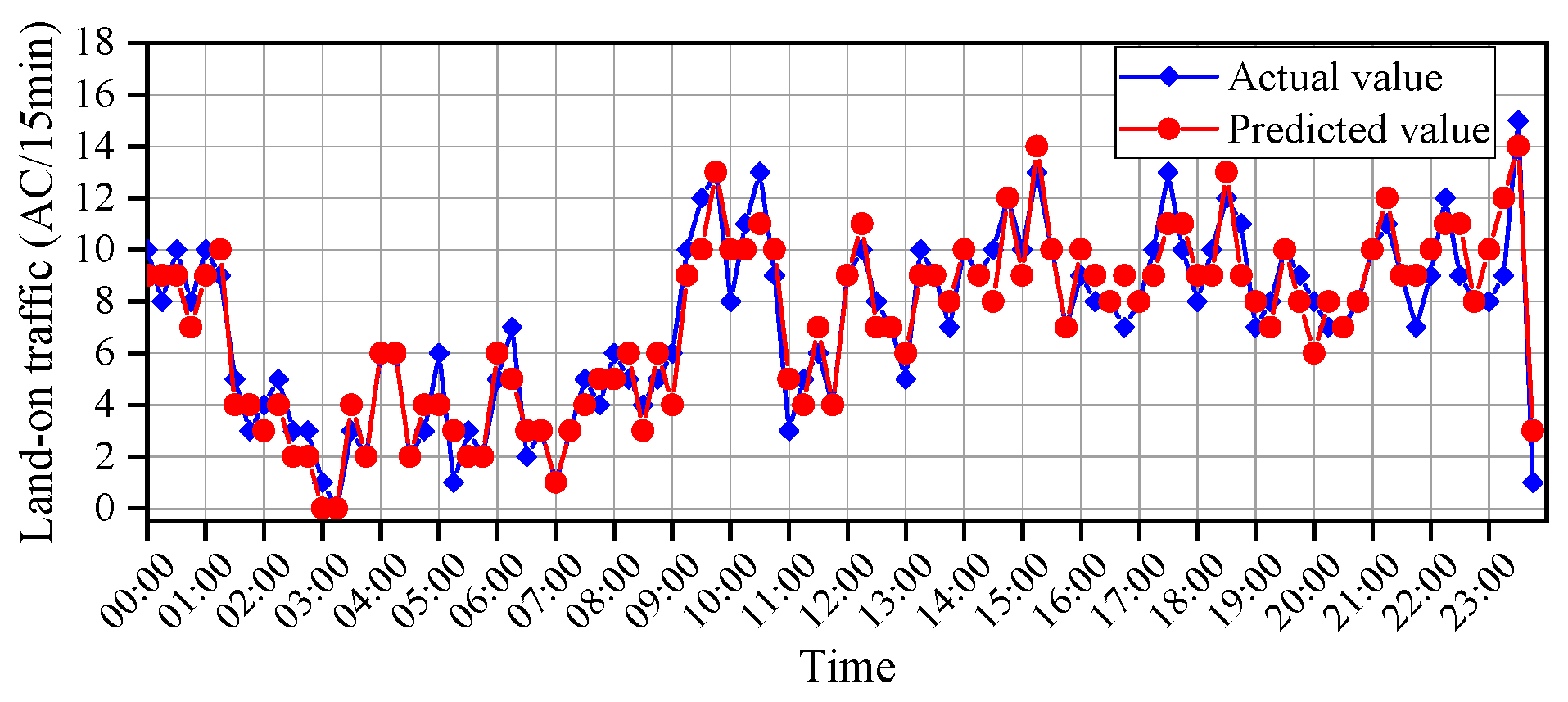
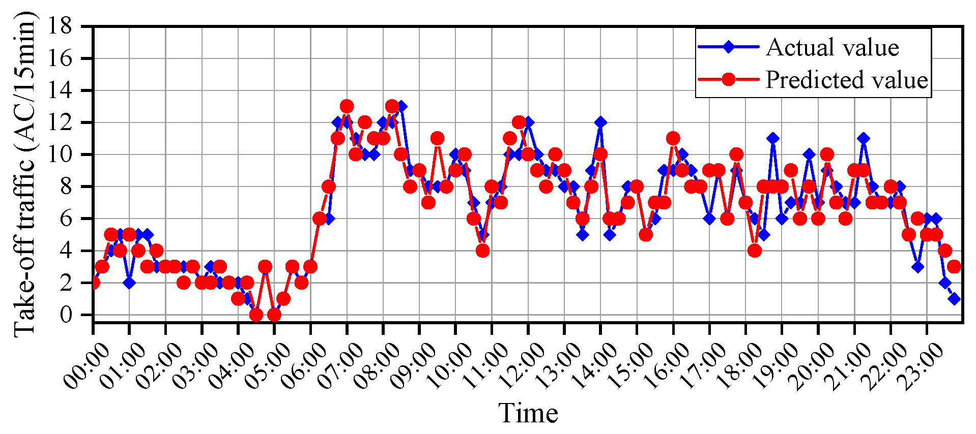
An airport’s land-on and take-off traffic values are crucial for assessing its operational efficiency and congestion levels. These values are defined as the number of aircraft landing and taking off from the runway within a specific time unit, passing through the terminal’s airspace. The comparison between simulated and actual data for the number of takeoffs and landings per unit time at ZSSS is shown in Figure 24 and Figure 25, respectively. For a 15 min interval, the MAE for the land-on traffic value at ZSSS is 0.68 AC/15 min, with a standard deviation of 0.60 AC/15 min. The MAE for take-off traffic is 0.78 AC/15 min, with a standard deviation of 0.65 AC/15 min. Similarly, the comparison for ZSPD is shown in Figure 26 and Figure 27. The MAE for the land-on traffic value at ZSPD is 0.86 AC/15 min, with a standard deviation of 0.66 AC/15 min, while the MAE for take-off traffic is 0.90 AC/15 min, with a standard deviation of 0.80 AC/15 min.
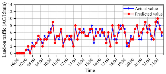
Figure 24.
The actual and predicted land-on traffic at ZSSS.

Figure 25.
The actual and predicted take-off traffic at ZSSS.

Figure 26.
The actual and predicted land-on traffic at ZSPD.

Figure 27.
The actual and predicted take-off traffic at ZSPD.
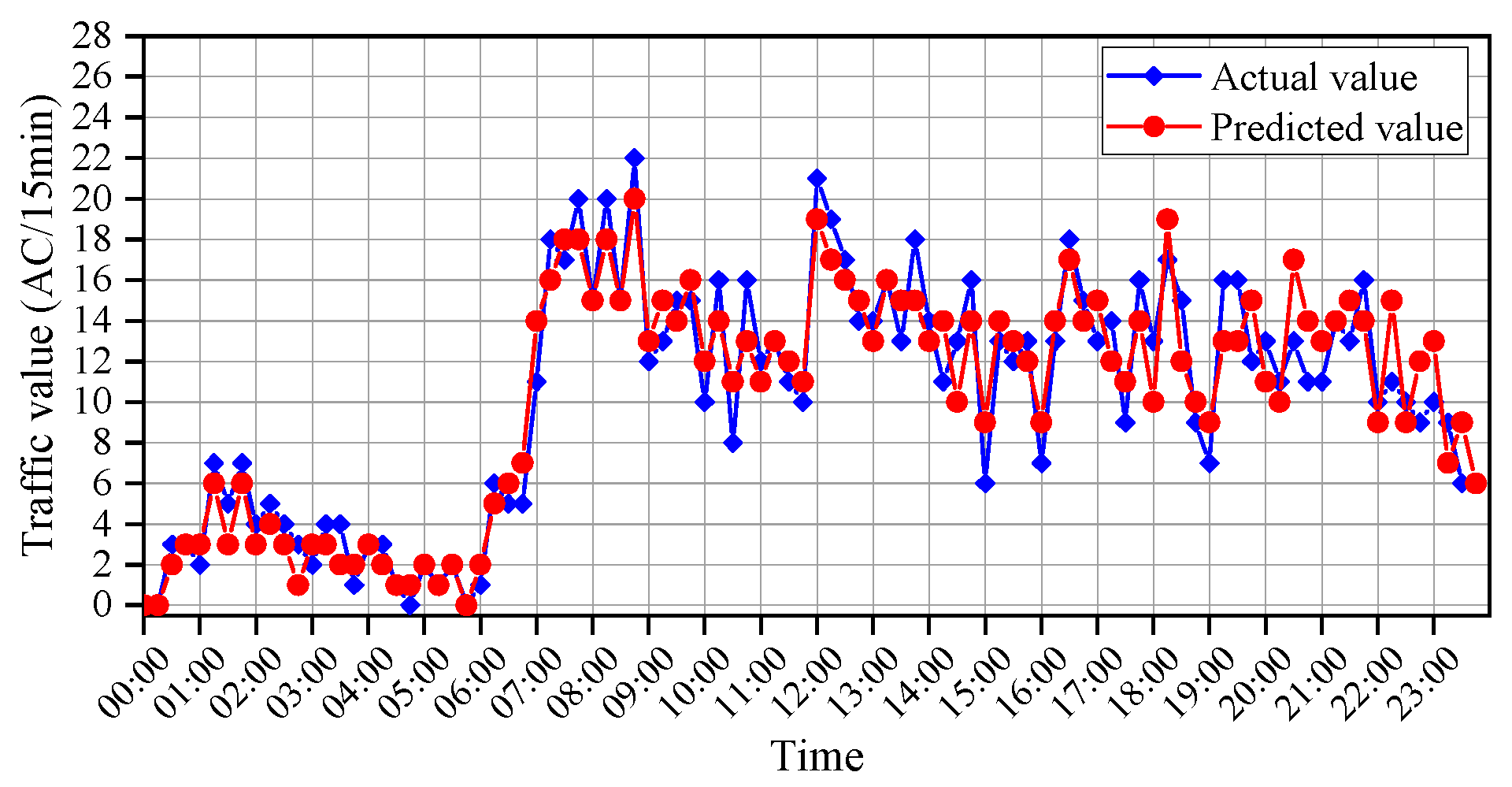
Next, we compare the simulated and actual traffic flow rates per unit of time across all departure fixes. Since the inbound traffic flow in the model validation is directly based on actual arrival times at the arrival fixes, there is no need to validate the inbound traffic values separately. As shown in Figure 28, the actual and simulated traffic values closely align at the 15 min scale, with only minor deviations observed in some periods. The overall MAE is 1.53 AC/15 min, with a standard deviation of 1.02 AC/15 min.

Figure 28.
The actual and predicted outflow at departure points.
In summary, we validate the integrated surface–airspace traffic model proposed in this study from two perspectives: operational time at different stages, and traffic values. The results show that the model is capable of simulating the traffic dynamics within multi-airport regions with acceptable accuracy.
4.4. Capacity Decoupling Analysis
Using the northbound operation mode of the Shanghai terminal area as the test scenario, the integrated surface–airspace traffic model for the Shanghai multi-airport region was employed to simulate the evolution of traffic dynamics. A Monte Carlo simulation-based capacity decoupling analysis was conducted, with historical flight operation data from July to December 2019 serving as the flight schedule database. This generated a total of 403 random flight schedules. The daily flights ranged from 1368 to 1691 for ZSPD and from 664 to 872 for ZSSS. Based on the relevant technical specifications published by the Civil Aviation Administration of China (CAAC), acceptable delay thresholds were set, including an average daily delay of no more than 8 min and a peak-hour average delay of no more than 15 min. Using hourly and 15 min intervals along with a 95% quantile, the coupling relationships between single-airport and multi-airport arrival and departure traffic were analyzed using the frequency-constrained quantile envelope model.
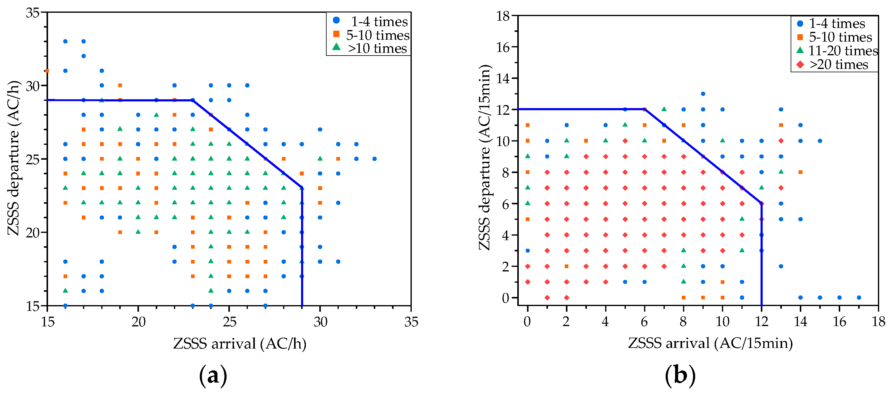
At the single-airport level, the envelope results for ZSSS are represented by the blue lines in Figure 29. In Figure 29a, scatter points of varying shapes represent distinct frequency categories of observed data: blue circles denote occurrences with frequencies of 1–4, orange squares correspond to frequencies of 5–10, and green triangles indicate frequencies exceeding 10. Figure 29b further classifies the frequency data into four categories (1–4, 5–10, 11–20, and >20), distinguished by four minunique marker types. The notation and line conventions apply to subsequent figures in this subsection.
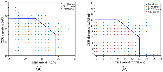
Figure 29.
Capacity envelope of arrival and departure traffic at ZSSS. (a) Hourly; (b) 15 min.
At ZSSS, a strong interdependence exists between arrival and departure traffic flows. The maximum hourly takeoff and landing capacity on the envelope curve is 52 AC/h, with the maximum hourly capacity for both arrivals and departures being 29 AC/h. The peak coupling intensity between arrival and departure traffic flows reaches 7 AC/h. At the 15 min interval, the peak capacity for ZSSS is 18 AC/15 min, with both arrival and departure peak capacities at 12 AC/15 min.
Notably, all displayed data points satisfy the delay criteria, as outliers were filtered according to Equation (22). However, sporadic points persist outside the envelope curve, predominantly representing low-frequency anomalies likely caused by transient traffic surges. These scenarios may reflect unstable operational states that cannot sustain long-term equilibrium. The quantile regression methodology in this paper was specifically adopted to enhance the robustness of the envelope analysis against such irregular observations, supporting airport capacity determination and slot allocation.
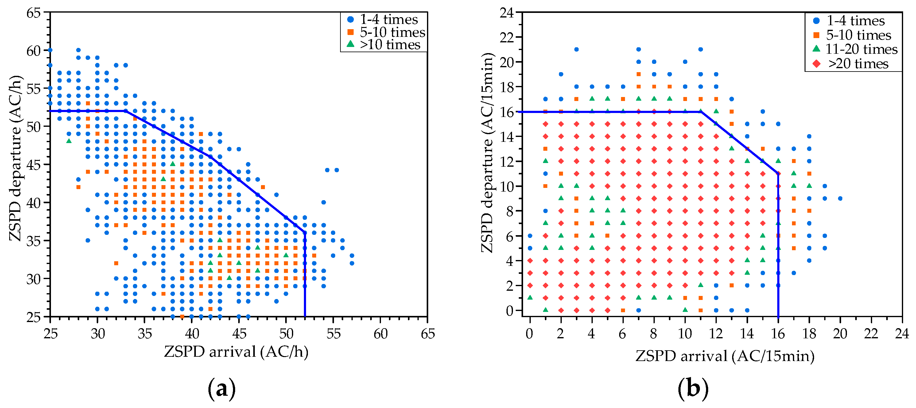
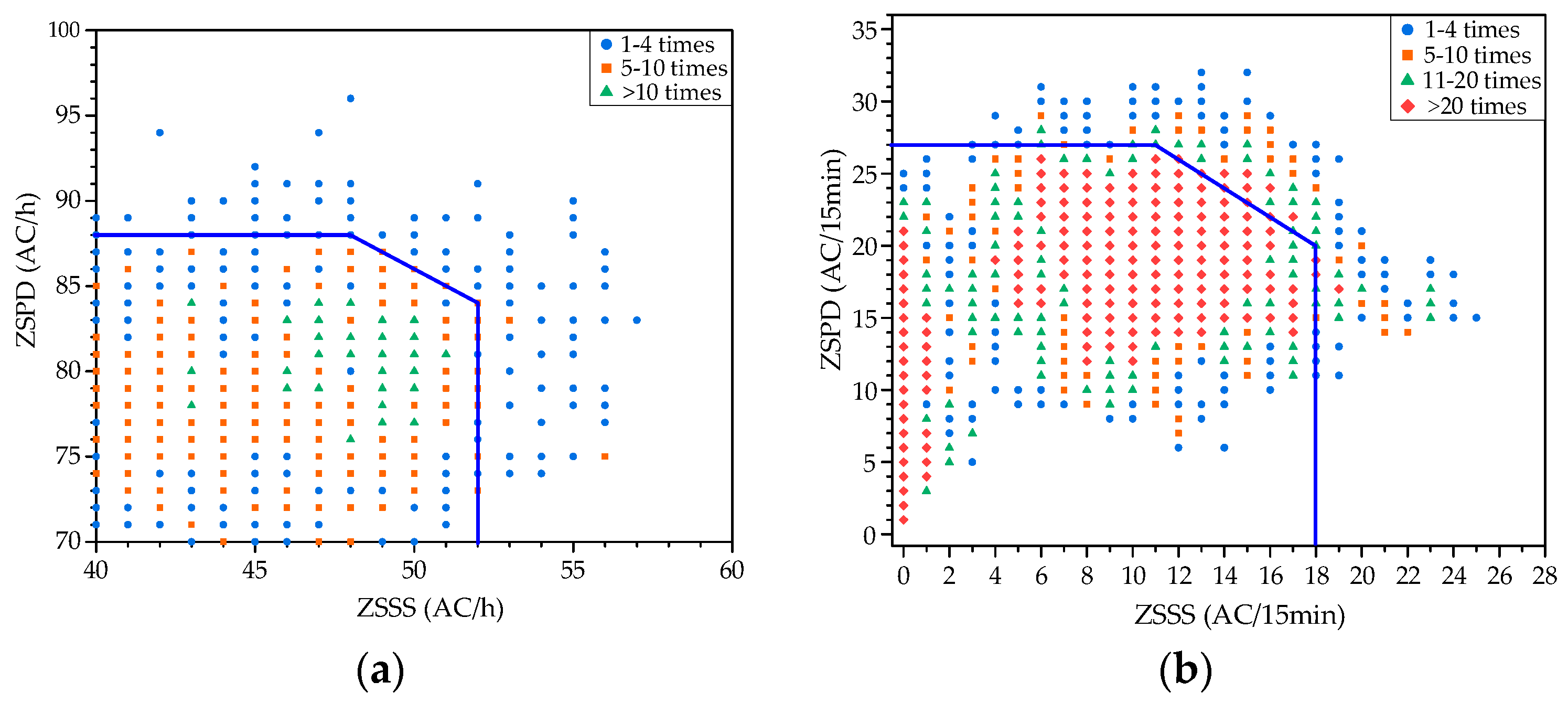
Figure 30 displays the envelope results for arrival and departure traffic flows at ZSPD. The statistical analysis of hourly capacity indicates that the interdependence between arrivals and departures at ZSPD is more pronounced than at ZSSS. The maximum sample point on the hourly capacity envelope is 88 AC/h, with peak service capacities for both arrivals and departures reaching 52 AC/h. The maximum sample point on the 15 min capacity envelope is 27 AC/15 min.
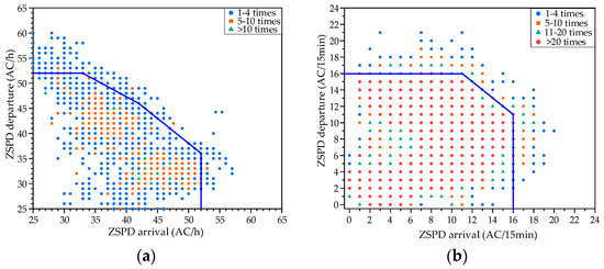
Figure 30.
Capacity envelope of arrival and departure traffic at ZSPD. (a) Hourly; (b) 15 min.
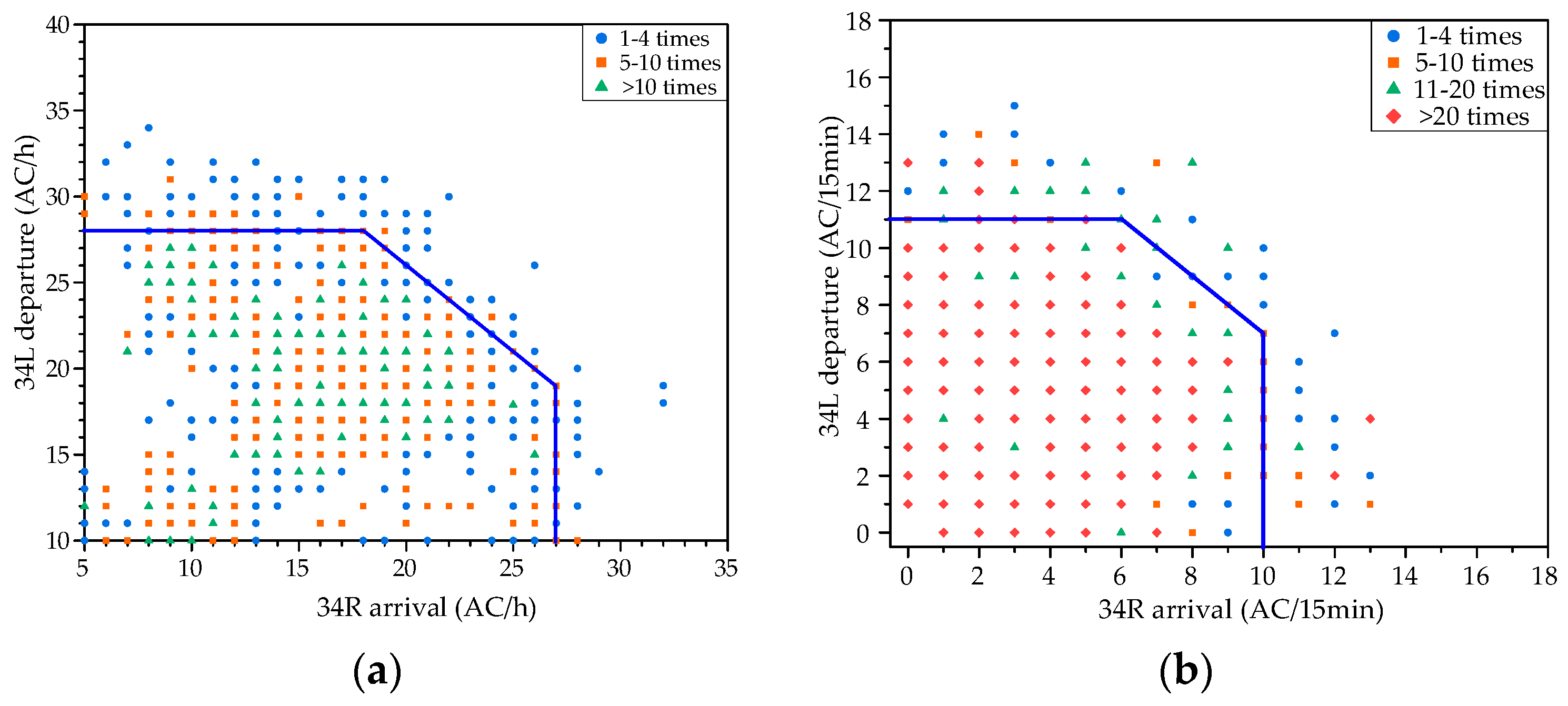
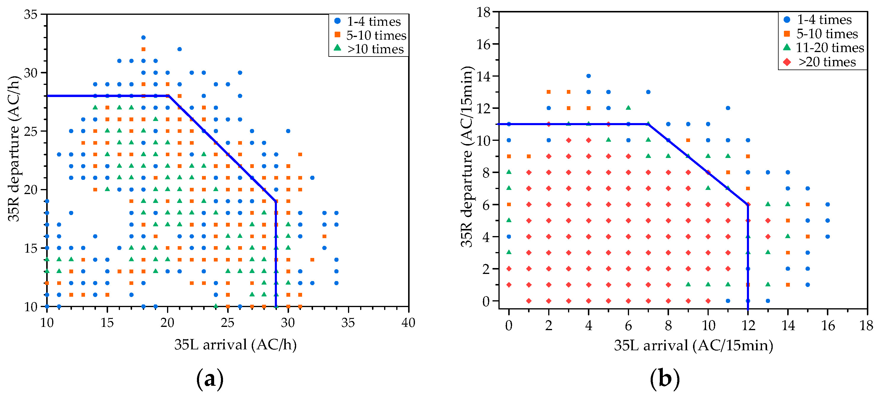
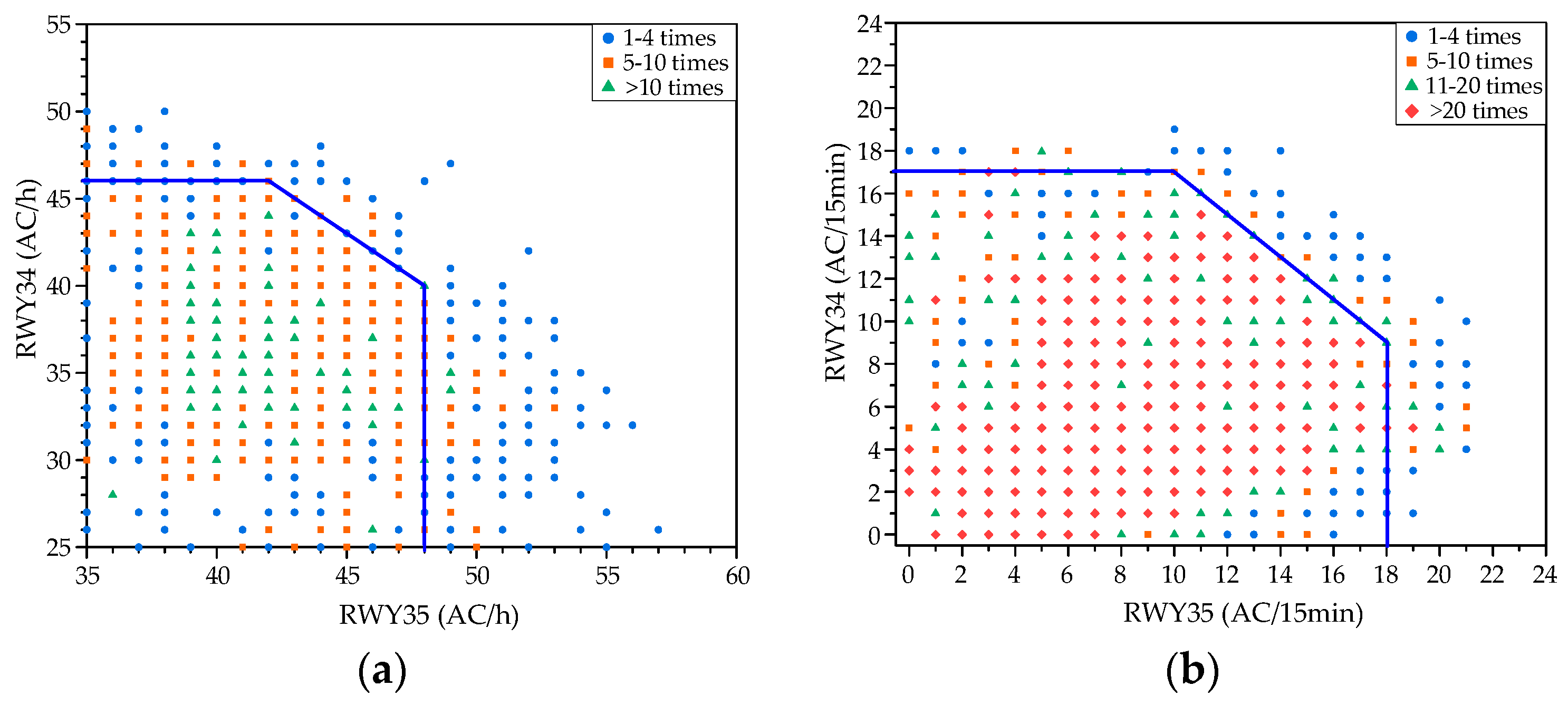
ZSPD features two pairs of parallel runways, with the coupling capacity between the east and west runways of Runway 34 and Runway 35 shown in Figure 31 and Figure 32. The interdependent relationship between arrival and departure flows is significant. Specifically, Runway 34R has a maximum landing rate of 27 AC/h, while Runway 34L has a maximum departure rate of 28 AC/h, with a maximum coupling intensity of 10 AC/h. Runway 35L has a maximum landing rate of 29 AC/h, and Runway 35R has a maximum departure rate of 28 AC/h.

Figure 31.
Capacity envelope of arrival and departure traffic on Runway 34 at ZSPD. (a) Hourly; (b) 15 min.

Figure 32.
Capacity envelope of arrival and departure traffic on Runway 35 at ZSPD. (a) Hourly; (b) 15 min.
In a 15 min interval, the maximum service capacities for landing runways 34R and 35L are 10 aircraft and 12 aircraft, respectively, while both departure runways 34L and 35R have a maximum capacity of 11 aircraft. Figure 33 illustrates the coupling effects between Runway 34 and Runway 35. At both the hourly and 15 min scales, the maximum capacity for Runway 34 is 46 AC/h and 17 AC/15 min, while for Runway 35, it is 48 AC/h and 18 AC/15 min.
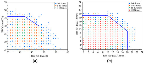
Figure 33.
Capacity envelope of Runway 34 and Runway 35 traffic at ZSPD. (a) Hourly; (b) 15 min.
At the multi-airport level, the interdependent relationship between the total arrival and departure flights at ZSSS and ZSPD is illustrated in Figure 34. Under balanced operations at both airports, the number of flights ranges from 48 to 52 AC/h at ZSSS and from 84 to 88 AC/h at ZSPD. The maximum coupling capacity for both airports is 136 AC/h. At a 15 min interval, the maximum capacity for ZSSS is 18 AC/15 min, for ZSPD it is 27 AC/15 min, and the combined maximum capacity for both airports is 38 AC/15 min.
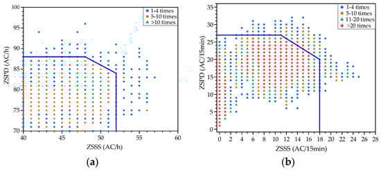
Figure 34.
Capacity envelope of ZSSS and ZSPD traffic. (a) Hourly; (b) 15 min.
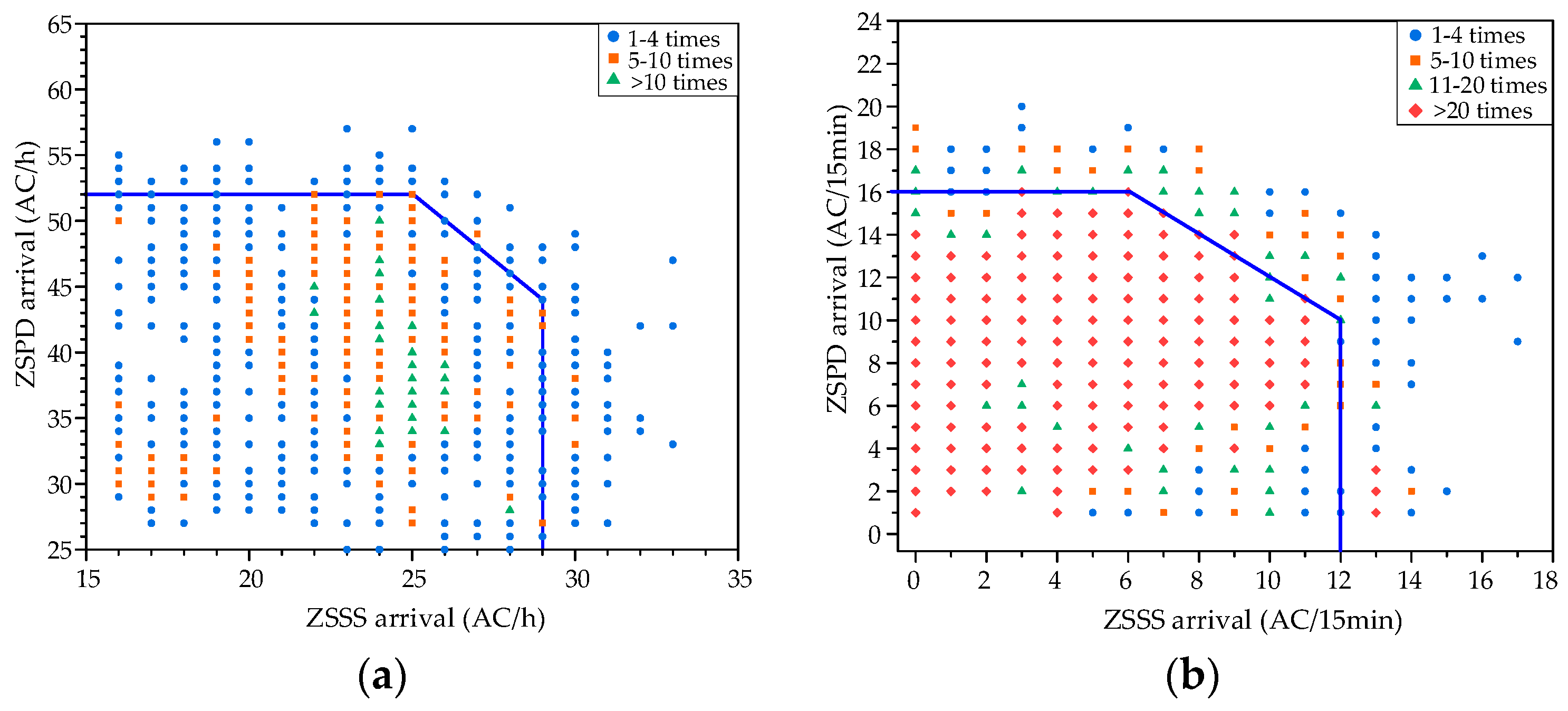
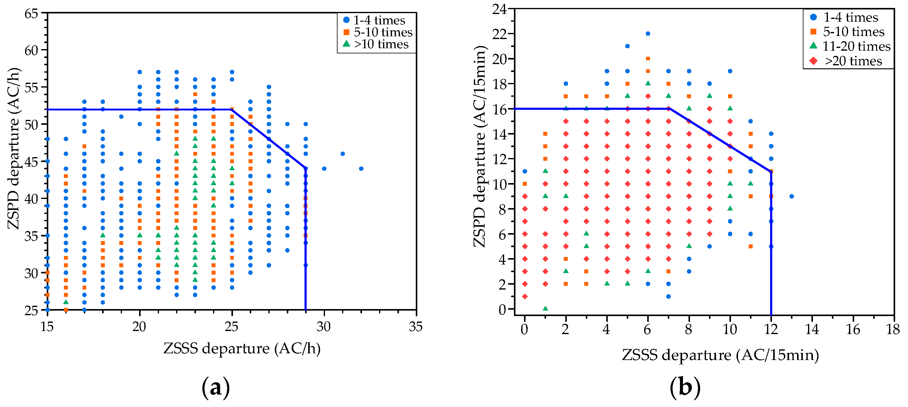
Next, we further explore the interdependence arising from resource competition within the multi-airport system by analyzing different combinations of arrival and departure traffic flows at these two airports. Figure 35 and Figure 36 present the coupling capacity envelopes for all arrival and departure traffic flows at the hourly and 15 min statistical scales, respectively. The curves show that a certain degree of coupling exists between departure and arrival traffic flows at both airports, reflecting the impact of shared resources such as route segments and departure/arrival fixes. The hourly capacity for arrival and departure flows in this multi-airport system is 77 AC/h, with the capacity at the 15 min interval being 22 AC/15 min and 23 AC/15 min, respectively.

Figure 35.
Capacity envelope of arrival traffic at ZSSS and ZSPD. (a) Hourly; (b) 15 min.
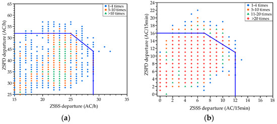
Figure 36.
Capacity envelope of departure traffic at ZSSS and ZSPD. (a) Hourly; (b) 15 min.
5. Summary
The high complexity and strong coupling of traffic within multi-airport regions pose significant challenges for air traffic flow management. This paper focuses on multi-airport coupled operations, addressing traffic modeling and capacity decoupling. We divide aircraft operations into surface taxiing and airspace flying. Using linear regression models with effective traffic values and random forest models with taxiing situation indices, we predict unimpeded taxiing time and taxiway network delays. We form the SRN based on SIFPs and dualize it with segments, runways, waypoints, and fixes as nodes. A fluid queue model is used for simulation within each node, and an inter-node traffic transmission mechanism is introduced. Based on this integrated traffic model, this study proposes a Monte Carlo-based capacity decoupling analysis method for multi-airport regions. The envelope, which reflects the dynamic capacity among various levels of traffic, is modeled using a quantile regression approach.
Additionally, this paper presents a case study of Shanghai, whereby the model is validated using experimental data and parameters. The results demonstrate that the model effectively simulates dynamic traffic flows within an acceptable margin of error. The study also explores the interdependence between arrival and departure traffic flows both within and between the two airports in the Shanghai multi-airport region.
The coupled and dynamic capacity for multi-airport regions developed in this study challenges the traditional fixed capacity value, offering a more accurate reflection of the interdependence between various airport traffic flows. This capacity decoupling analysis provides essential insights for determining coordination parameters and optimizing flight slot allocation in multi-airport systems. Furthermore, traffic management department can dynamically allocate airport resources within the capacity limits, effectively balancing demand and operational efficiency.
In future research, we will further explore the dynamic aspects of the operational environment in multi-airport regions, including time-varying service capacities. Additionally, we aim to simplify the integrated surface–airspace traffic model to enhance its applicability to larger airport networks. From a capacity and demand management perspective, we will also investigate more control measures to address the interdependence arising from resource sharing between airports.
Author Contributions
Conceptualization, L.Y., Y.W. and Y.R.; methodology, L.Y., Y.W., S.W. and S.L.; software, Y.W., M.W. and S.W.; validation, Y.R., S.L. and S.W.; formal analysis, S.L. and S.W.; investigation, S.W. and Y.R.; writing—original draft preparation, L.Y. and Y.W.; writing—review and editing, S.W. and L.Y.; supervision, L.Y.; project administration, L.Y.; funding acquisition, L.Y. All authors have read and agreed to the published version of the manuscript.
Funding
This research was funded by the Natural Science Foundation of Jiangsu Province (BK20231447) and the National Natural Science Foundation of China (52472346).
Data Availability Statement
The datasets presented in this article are not readily available because the data are part of an ongoing study. Requests to access the datasets should be directed to the Civil Aviation Administration of China.
Conflicts of Interest
The authors declare no conflicts of interest.
References
- Caccavale, M.V.; Iovanella, A.; Lancia, C.; Lulli, G.; Scoppola, B. A Model of Inbound Air Traffic: The Application to Heathrow Airport. J. Air Transp. Manag. 2014, 34, 116–122. [Google Scholar] [CrossRef]
- Itoh, E.; Mitici, M.; Schultz, M. Modeling Aircraft Departure at a Runway Using a Time-Varying Fluid Queue. Aerospace 2022, 9, 119. [Google Scholar] [CrossRef]
- Ramanujam, V.; Balakrishnan, H. Estimation of Arrival-Departure Capacity Tradeoffs in Multi-Airport Systems. In Proceedings of the 48h IEEE Conference on Decision and Control (CDC) Held Jointly with 2009 28th Chinese Control Conference, Shanghai, China, 15–18 December 2009; pp. 2534–2540. [Google Scholar]
- Schultz, M.; Reitmann, S.; Alam, S. Predictive Classification and Understanding of Weather Impact on Airport Performance through Machine Learning. Transp. Res. Part C Emerg. Technol. 2021, 131, 103119. [Google Scholar] [CrossRef]
- Lui, G.N.; Hon, K.K.; Liem, R.P. Weather Impact Quantification on Airport Arrival On-Time Performance through a Bayesian Statistics Modeling Approach. Transp. Res. Part C Emerg. Technol. 2022, 143, 103811. [Google Scholar] [CrossRef]
- Janic, M. Modeling Effects of Different Air Traffic Control Operational Procedures, Separation Rules, and Service Disciplines on Runway Landing Capacity. J. Advced Transp. 2014, 48, 556–574. [Google Scholar] [CrossRef]
- Blumstein, A. The Landing Capacity of a Runway. Oper. Res. 1959, 7, 752–763. [Google Scholar] [CrossRef]
- Mascio, P.D.; Rappoli, G.; Moretti, L. Analytical Method for Calculating Sustainable Airport Capacity. Sustainability 2020, 12, 9239. [Google Scholar] [CrossRef]
- Janić, M. Transport Systems: Modelling, Planning, and Evaluation, 1st ed.; CRC Press: Boca Raton, FL, USA, 2016; ISBN 978-1-315-37102-3. [Google Scholar]
- Wang, L.; Li, H.; Zhang, Z. Evaluation of Approach Runway Capacity under Medium Heavy Aircraft Combination. In Proceedings of the 2023 7th International Seminar on Education, Management and Social Sciences (ISEMSS 2023); Yacob, S., Cicek, B., Rak, J., Ali, G., Eds.; Advances in Social Science, Education and Humanities Research. Atlantis Press SARL: Paris, France, 2023; Volume 779, pp. 1401–1408, ISBN 978-2-38476-125-8. [Google Scholar]
- Gilbo, E.P. Airport Capacity: Representation, Estimation, Optimization. IEEE Trans. Contr. Syst. Technol. 1993, 1, 144–154. [Google Scholar] [CrossRef] [PubMed]
- Ju, F.; Cai, K.; Yang, Y.; Gao, Y. A Scenario-Based Optimization Approach to Robust Estimation of Airport Capacity. In Proceedings of the 2015 IEEE 18th International Conference on Intelligent Transportation Systems, Gran Canaria, Spain, 15–18 September 2015; pp. 2066–2071. [Google Scholar]
- Abdelghani, F.; Cai, K.; Zhang, M. A Chance-Constrained Optimization Approach for Air Traffic Flow Management Under Capacity Uncertainty. In Proceedings of the 2022 Integrated Communication, Navigation and Surveillance Conference (ICNS), Dulles, VA, USA, 5–7 April 2022; pp. 1–11. [Google Scholar]
- Badrinath, S.; Li, M.Z.; Balakrishnan, H. Integrated Surface–Airspace Model of Airport Departures. J. Guid. Control Dyn. 2019, 42, 1049–1063. [Google Scholar] [CrossRef]
- Menon, P.K.; Sweriduk, G.D.; Bilimoria, K.D. New Approach for Modeling, Analysis, and Control of Air Traffic Flow. J. Guid. Control Dyn. 2004, 27, 737–744. [Google Scholar] [CrossRef]
- Sun, D.; Bayen, A.M. Multicommodity Eulerian-Lagrangian Large-Capacity Cell Transmission Model for En Route Traffic. J. Guid. Control Dyn. 2008, 31, 616–628. [Google Scholar] [CrossRef]
- Bayen, A.M.; Raffard, R.L.; Tomlin, C.J. Adjoint-Based Control of a New Eulerian Network Model of Air Traffic Flow. IEEE Trans. Contr. Syst. Technol. 2006, 14, 804–818. [Google Scholar] [CrossRef]
- Roy, S.; Sridhar, B.; Verghese, G.C. An Aggregate Dynamic Stochastic Model for an Air Traffic System. In Proceedings of the 5th Eurocontrol, Budapest, Hungary, 23–27 June 2003. [Google Scholar]
- Iwata, D.; Itoh, E. Developing Aircraft Departure Queueing Models for a Mixed Takeoff/Landing Operational Runway. In 2023 Asia-Pacific International Symposium on Aerospace Technology (APISAT 2023) Proceedings; Fu, S., Ed.; Lecture Notes in Electrical Engineering; Springer: Singapore, 2024; Volume 1050, pp. 555–570. ISBN 978-981-97-3997-4. [Google Scholar]
- Itoh, E.; Mitici, M. Queue-Based Modeling of the Aircraft Arrival Process at a Single Airport. Aerospace 2019, 6, 103. [Google Scholar] [CrossRef]
- Wang, S.; Yang, L.; Wang, Y.; Cong, W. A Data and Model-Driven Approach to Predict Congestion of Departure Traffic at Airport. In Proceedings of the 2022 Integrated Communication, Navigation and Surveillance Conference (ICNS), Dulles, VA, USA, 5–7 April 2022; pp. 1–15. [Google Scholar]
- Simaiakis, I.; Balakrishnan, H. Queuing Models of Airport Departure Processes for Emissions Reduction. In Proceedings of the AIAA Guidance, Navigation, and Control Conference, Chicago, IL, USA, 10–13 August 2009. [Google Scholar]
- Yang, L.; Wang, S.; Liang, F.; Zhao, Z. A Holistic Approach for Optimal Pre-Planning of Multi-Path Standardized Taxiing Routes. Aerospace 2021, 8, 241. [Google Scholar] [CrossRef]
- Idris, H.; Clarke, J.-P.; Bhuva, R.; Kang, L. Queuing Model for Taxi-Out Time Estimation. Air Traffic Control Q. 2002, 10, 1–22. [Google Scholar] [CrossRef]
- Yin, J.; Hu, M.; Ma, Y.; Han, K.; Chen, D. Airport Taxi Situation Awareness with a Macroscopic Distribution Network Analysis. Netw. Spat. Econ. 2019, 19, 669–695. [Google Scholar] [CrossRef]
- Lee, H.; Malik, W.; Jung, Y.C. Taxi-Out Time Prediction for Departures at Charlotte Airport Using Machine Learning Techniques. In Proceedings of the 16th AIAA Aviation Technology, Integration, and Operations Conference, Washington, DC, USA, 13–17 June 2016. [Google Scholar]
- Whitt, W. Fluid Models for Multiserver Queues with Abandonments. Oper. Res. 2006, 54, 37–54. [Google Scholar] [CrossRef]
- Newell, G.F. Airport Capacity and Delays. Transp. Sci. 1979, 13, 179–268. [Google Scholar] [CrossRef]
- Yang, L.; Yin, S.; Hu, M.; Han, K.; Zhang, H. Empirical Exploration of Air Traffic and Human Dynamics in Terminal Airspaces. Transp. Res. Part C Emerg. Technol. 2017, 84, 219–244. [Google Scholar] [CrossRef]


Disclaimer/Publisher’s Note: The statements, opinions and data contained in all publications are solely those of the individual author(s) and contributor(s) and not of MDPI and/or the editor(s). MDPI and/or the editor(s) disclaim responsibility for any injury to people or property resulting from any ideas, methods, instructions or products referred to in the content. |
© 2025 by the authors. Licensee MDPI, Basel, Switzerland. This article is an open access article distributed under the terms and conditions of the Creative Commons Attribution (CC BY) license (https://creativecommons.org/licenses/by/4.0/).