Abstract
Aero-engine performance monitoring is a core component of the engine health management system and an important approach to enhancing flight safety and reliability. Meanwhile, to improve engine operation efficiency, control systems are evolving from traditional centralized architectures to distributed control architectures. To alleviate the negative impact of network uncertainties, this paper proposes a Distributed Adaptive Kalman Filter (DAKF), which resolves the estimation performance degradation of the classical Kalman Filter under network uncertainty by designing measurement reconstruction and buffer-based signal fusion strategies, expanding the engineering applicability of the Kalman Filter in distributed control architectures. Furthermore, a distributed hardware architecture was established based on the time-triggered protocol/class (TTP/C) bus protocol, communication programs between simulation nodes were developed, and the proposed DAKF algorithm was deployed in the hardware architecture for experimental validation. This study focuses on the steady-state operations of the turboshaft engine to investigate the performance of the proposed distributed Kalman Filter algorithm under network uncertainties. The results demonstrated the effectiveness of the proposed method, providing a basis for the engineering application of distributed performance monitoring methods.
1. Introduction
1.1. Motivation
Aero-engines usually have complex structures and face harsh operating environments. Thus, their operational reliability is critical to flight safety. Statistical data show that engine failures can lead to serious flight accidents and even trigger catastrophic disasters [1]. Current development trends indicate that the maintenance principle of aircraft engines is gradually evolving from “prevention-oriented” to “reliability-oriented”. Timely monitoring of engine performance is fundamental to eliminating risks and ensuring flight safety, as well as reducing engine lifecycle maintenance costs. Therefore, monitoring and analyzing the performance of the aero-engine gas path components is of great significance [2].
Currently, engine performance analysis methods can be primarily categorized into three types: model-based [3], data-driven [4], and knowledge-experience-based methods [5]. Among these, model-based performance analysis uses the engine model output as a benchmark to determine the difference between actual sensor outputs and the benchmark. By analyzing this difference, changes in component performance can be deduced. This method has been widely applied irrespective of data sample limitations. In numerous studies, the Kalman Filter is one of the more mature methods currently used. Traditionally, the implementation of the Kalman Filter is based on a centralized architecture, wherein a singular filter processes all sensor data. This approach is preeminent in structural simplicity and ease of implementation; however, it may lead to a significant computational burden on the central processor, complex communication lines, and limited sensor fault tolerance. With an advancement in distributed control technology, intelligent sensors, intelligent actuators, and high-speed bus technologies are gradually being applied to engines, providing favorable conditions for distributed filtering estimation structures for engine gas path performance. Distributed filtering methodologies leverage a network of sub-filters to independently process their respective measurement data in parallel, formulating a global algorithm to synthesize the local estimation outputs from these sub-filters into a comprehensive global result. Sub-filters are constructed independently, offering advantages such as high scalability, reduced computational burden on the central processor, and simplified communication lines. Therefore, this paper studies the distributed filtering method for a turboshaft engine.
However, the rise of network control system architectures has also introduced increased uncertainties during the retransmission of various sensor signals. For instance, when the data network communication is congested or excessively harsh, blockages and interruptions may occur during data transmission, leading to packet loss. Although significant research has been conducted on the uncertainty of measurement signal transmission, little attention has been paid to the issue of packet loss on the state signal end. This issue can severely impact the reliability of aircraft engine control and performance monitoring systems. Therefore, it is essential to research the uncertainties in distributed control architecture networks.
On the other hand, current research on aircraft engine state estimation mostly remains at the simulation level. For distributed network systems, digital simulation alone is insufficient to meet the validation requirements, as it lacks the capability to simulate hardware characteristics and signal transmission scenarios. Therefore, this paper establishes a distributed hardware architecture based on the TTP/C communication protocol and deploys distributed performance monitoring methods onto this hardware architecture for experimentation. This aims to provide a foundation for the engineering application of distributed performance monitoring methods.
1.2. Literature Review
The engine health management (EHM) system aims to assess the engine’s health status using sensor data, evaluate the engine’s condition, detect and locate existing faults, and integrate resource information to achieve condition-based maintenance of the engine [6]. Given that gas path component faults are the most typical failures, diagnosing these faults is of crucial importance to the EHM system [7]. Model-based filters [8] and data-driven intelligent algorithms [9] are the two most common methods. Though each method has particular advantages under different conditions, both of them require sufficient measurement information to assess the current health status of the air system. Moreover, due to the harsh operating environment of the engine, the number and location of sensors installed on the engine are limited. Therefore, efficiently utilizing the available sensor data to achieve health management functions is a highly valuable issue. The concept of engine health management emerged in the late 1960s and was first applied to civil engines in the 1970s, significantly enhancing flight safety and operational efficiency. Since the 21st century, engine health management technology has been widely adopted. In the IHPTET program, which was concluded in 2005, the application of this technology led to a reduction in engine production and maintenance costs by 32% and 31%, respectively. Condition monitoring and fault diagnosis are the primary functions of an engine health management system, particularly for gas path component faults. Statistics indicate that maintenance costs associated with gas path component faults account for approximately 60% of the total engine maintenance expenses.
Early gas path fault diagnosis relied on the Kalman Filter. As application scenarios and objects have become increasingly complex, a variety of derivative algorithms have emerged in succession. Considering the numerical stability and accuracy of filtering estimates caused by system uncertainties, Chen et al. [10] enhanced the Spherical Unscented Kalman Filter (SUKF) algorithm by incorporating correction factors and offline calibration strategies. Liu et al. [11] addressed the problem of limited sensor data relative to unknown health parameters by developing an underdetermined Extended Kalman Filter (EKF), accompanied by formal proof of its convergence. To improve the accuracy of health parameter estimation using limited sensor data, Wang et al. proposed integrating measurement parameter selection optimization with the Kalman Filtering algorithm [12]. Chen et al. [13] proposed an optimization method based on correlation and condition number for selecting health parameters in turboshaft engines. Traditional Kalman Filters struggle to estimate states accurately when the number of measurement sensors does not match the health parameters. To resolve this, Liu et al. [14] introduced a neural network-enhanced Kalman Filter, significantly improving estimation accuracy.
With the development of computer technology, neural networks have been widely used to estimate engine health parameters. To address the challenge of fault data arising from diverse operating conditions in turboshaft engines, Zhao et al. [15] proposed two transfer learning methods based on extreme learning machines (ELMs). Yu et al. [16] employed principal component analysis (PCA)-based dimensionality reduction in combination with an improved clustering algorithm to suppress noise interference during fault feature extraction for turboshaft engines.
As aircraft engines continue to evolve, there are increasing demands on the control systems to meet the needs for higher thrust-to-weight ratios and improve their economic performance, requiring higher standards for the system’s size, weight, quality assurance, and research and development costs. Distributed control architecture can reduce the system’s size and weight, while enhancing its versatility and reliability, as well as lowering maintenance costs. Compared to the traditional centralized architectures, distributed architectures are more efficient, and their modular design also makes system upgrades easier [17,18]. However, in the distributed control architectures, network uncertainties such as transmission delays and data packet loss are unavoidable, since the smart sensor nodes, intelligent actuators, and central control nodes are connected through a data bus. These issues may occur at various stages of data transmission over the bus and can negatively impact both control and health management system, leading to instability, thereby compromising the engine system’s operational reliability and safety. Therefore, research on the network uncertainties of distributed control architecture is highly necessary.
New filtering methods are emerging to address the new challenges posed by network communication issues. To alleviate the burden on network communication, Ribeiro et al. [19] proposed a distributed state estimation recursive algorithm based on residual marking. To reduce the computational load on each node and improve network fault tolerance, Chen [20] introduced a finite-time federated filter. For the issue of multi-rate sensor network systems, Safari [21] designed a new sensor fusion algorithm based on neural network state estimation methods. Mahmoud [22], to address the delay effects in asynchronous multi-sensor systems, studied performance monitoring methods under delay and measurement loss conditions. Liu [23] designed a distributed sensing method to reduce the impact of measurement disturbances on state estimation accuracy. Olfati et al. [24,25] designed a distributed Kalman Consensus Filter (KCF), which calculates the optimal estimates of subsystems within sub-filters and then exchanges estimation results between the sub-filters to compute the global state estimate of the system. Kamal et al. [26] developed a generalized KCF method to improve the robustness of state estimation when nodes are inaccurate. These studies provide a theoretical basis for the engineering application of distributed filtering.
With the advancement of sensor measurement technologies, the issue of inaccurate filtering estimation caused by measurement uncertainties has garnered increasing attention. For the linear Kalman Filters with data packet losses occurring on both sides, the filters’ stability was investigated in [27,28,29]. In addition, some research has focused on robust Kalman Filtering algorithms aimed at improving the accuracy of state estimation in systems with random sensor delays and multiple packet losses [30,31]. For linear discrete-time varying systems constrained by bounded uncertainties, Rezaei [32] proposed a finite-time horizon robust Kalman Filtering algorithm, where measurements can be received through a packet-delaying network. Another approach involves introducing buffers into the filtering algorithm. Schenato [33] proposed a scheme using a fixed-length data buffer to address data delay and packet loss in state estimation for multi-sensor systems. This method is easy to implement and imposes a relatively small computational burden. Rezaei [34] modeled the data delay and packet loss between sensors and filters according to a Bernoulli distribution and proposed robust filtering estimation algorithms for multi-sensor network systems. Nikfetrat [35] addressed the problem of measurement data delay and packet loss between sensors and filters by modeling the delay and loss using random variables that follow an uncertain probability Bernoulli distribution. The filter gain was adjusted through an adaptive factor determined by the residual covariance, thereby improving estimation accuracy. Additionally, some scholars have proposed using finite-length buffers to handle measurement data delay and packet loss strategies, while analyzing the relationship between estimation stability and the data arrival process [36,37]. Based on this, further research has integrated buffers with federated filtering algorithms, proposing a fusion estimation method for networked systems experiencing packet loss and delay [38].
1.3. The Main Contribution of This Paper
Performance monitoring of aircraft engines is crucial for enhancing the safety and reliability of flight operations. Concurrently, the advancement of distributed architectures has significantly contributed to improving engine control and health management systems. However, the inevitable occurrence of various network uncertainties during bus data transmission can, in severe cases, lead to system instability, thereby jeopardizing engine operation. Therefore, this paper focuses on the performance monitoring method under the distributed control architecture of turboshaft engines, proposing an adaptive filtering algorithm tailored for distributed architectures and validating it through a hardware platform. This paper makes three primary contributions:
(1) A Kalman Filter suitable for distributed systems has been designed. Leveraging its modular advantages, it reduces the computational load on the central processor while enhancing the system’s fault tolerance.
(2) Aiming to deal with sensor data packet loss, an adaptive filtering strategy has been proposed. By reconstructing the lost data on both sides and designing a fusion method based on a state buffer, the degradation in estimation accuracy caused by data packet loss has been mitigated.
(3) Based on the TTP/C communication protocol, a distributed control architecture simulation platform incorporating a central control node, intelligent simulation node, data processing node, and data monitoring node has been established. The engine model and filter are deployed on this platform to perform experimental validation.
The review of current research has found extensive work on aero-engine performance monitoring, making significant contributions to theoretical development and practical applications. However, several challenges remain unresolved. Regarding the uncertainty in signal transmission for engine performance monitoring, these studies primarily focus on robust Kalman algorithm design to enhance state estimation accuracy in systems with random sensor delays and packet losses. These methods, predominantly based on passive estimation, tend to compromise algorithm performance to some extent and fail to utilize measurement signals fully. In contrast, the approach proposed in this study employs measurement reconstruction to establish mathematical models for signals with packet loss received by intelligent simulation nodes. Furthermore, our filtering algorithm incorporates data caching technology to store historical data through intelligent nodes. This strategy not only offers easy implementation but also imposes a relatively lower computational burden.
2. Network Uncertainty Analysis of the Distributed Control Architecture
2.1. Distributed Kalman Filter
In the field of aero-engine fault diagnosis, the Kalman Filter algorithm can be utilized for engine performance monitoring. This method employs a mathematical model of the aero-engine in conjunction with sensor measurement data to estimate the engine’s state, and it has achieved a relatively mature level of application. Kalman Filtering is used to estimate the minimum variance in a system state with real-time measurement information, assuming that the mathematical model of a nonlinear research plant is represented as follows [39]:
where is the state vector of the system, represents the control parameters, represents the measurements, and and are the process noise and measurement noise, respectively, which are generally assumed to be zero-mean white noise with uncorrelated normal distribution. and represent the state transition equation and measurement equation of the plant. Equation (1) represents the nonlinear model of a turboshaft engine, expressed in an implicit form due to the engine’s inherently high nonlinearity. In this work, a component-level model is employed. Detailed component calculation formulae and co-working equations can be found in [39,40].
The classical Kalman Filtering algorithm was designed for linear systems, while the Extended Kalman Filter transforms a nonlinear problem into an approximate linear problem through the Taylor expansion. Thus, for the nonlinear system described in Equation (1), the calculation procedures of the EKF are as follows:
- (a)
- Time update:
- (b)
- Measurement update:where and are the covariance matrixes of and . The Jacobian matrixes A and C are calculated as follows:
This present algorithm is predominantly utilized in centralized systems. However, for distributed architecture, it is designed based on a modular architecture, comprising intelligent sensor nodes, intelligent actuator nodes, and central control nodes, all interconnected via a data bus for information transmission. These components are characterized as “intelligent” due to their embedded processing capabilities, autonomous decision-making functions, and communication features, enabling local data acquisition and processing, execution of local algorithms, status monitoring, and fault diagnosis, thereby reducing the computational load on the central processing unit.
In the distributed performance monitoring system developed in this research, the architecture incorporates two distinct types of intelligent nodes: (1) simulation nodes dedicated to sub-filter computation and (2) central control nodes responsible for result fusion. The system architecture strategically positions the sub-filters within the intelligent simulation nodes to perform decentralized state estimation, while the fusion center is implemented in the central control node to integrate the local estimation outcomes. This architectural design demonstrates several significant advantages, including enhanced system flexibility, optimized resource-sharing capabilities, streamlined structural configuration, reduced maintenance requirements, and minimized computational burden on the central processing unit.
In the distributed filtering algorithm, each sub-filter adopts the Kalman Filter and uses part of the measurements to calculate the local posterior estimation and local error covariance matrix and then uploads them to the data bus. The central control node calculates a fused global state posterior estimation and global error covariance matrix. Then, the assigned information is returned to the intelligent nodes through the bus.
The calculation process of the distributed Kalman Filter is as follows. First, each sub-filter is updated according to Equation (5).
where the subscript i indicates the number of the sub-filter and and are the measurement matrixes corresponding to the i-th sub-filter.
After each sub-filter completes its local estimation, the local estimation results and are transmitted to the fusion center of the central control node. The covariance intersection algorithm is then employed to perform information fusion, yielding the global estimation results and . Subsequently, the results are distributed and uploaded to the data bus, where they await reception by the intelligent simulation nodes. The procedures of the central control node are as follows.
- (a)
- Information fusion:
- (b)
- Information distribution:
where M indicates the number of sun-filters and is the weight coefficient which satisfies the information conservation . Generally, is set as . When the intelligent simulation node where the sub-filter is located fails, the CPU will receive a fault indication signal. The fault sub-filter corresponding to will be set to zero, while the weight coefficients of the rest of the sub-filters are redistributed to meet the information conservation.
2.2. Data Packet Dropout Problem Under the Network Control
Under the distributed architecture, the sub-filters and the fusion center are deployed on different hardware nodes. Network uncertainties may arise when data are transmitted between these hardware nodes. These uncertainties include data packet dropout, transmission delay, and network attacks. This paper primarily focuses on the data packet dropout, which will cause delays in filter estimation responses. As the packet dropout rate increases, the accuracy of the estimation declines and eventually diverges. For this work, the packet dropout is supposed to follow the random Bernoulli distribution.
Figure 1 illustrates potential points of data packet dropout, where the red arrow indicates that the data there were lost during the transmission. The dropout can be categorized into three situations: (a) Sensor data dropout—the intelligent simulation node fails to receive measurement information, causing the performance monitor to use the last received measurements for estimation. (b) Local estimation result dropout—the central control node fails to receive sub-filter estimation results, causing it to use the last received local estimation result. (c) Information distribution dropout—the global estimation result fails to update sub-filters, causing the sub-filter to rely on the last available information distribution result.
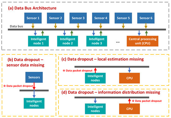
Figure 1.
Data packet dropout under distributed architecture.
Aiming at the data packet dropout, this paper proposes an improved Distributed Adaptive Kalman Filter (DAKF) method, which uses the reconstructed measurements to update the sub-filters in real time. Meanwhile, a state buffer is added to the central control node to handle the local estimation dropout and achieve accurate performance monitoring results.
3. Performance Monitoring Based on the Improved Distributed Adaptive Kalman Filter
3.1. Distributed Performance Monitoring of the Turboshaft Engine
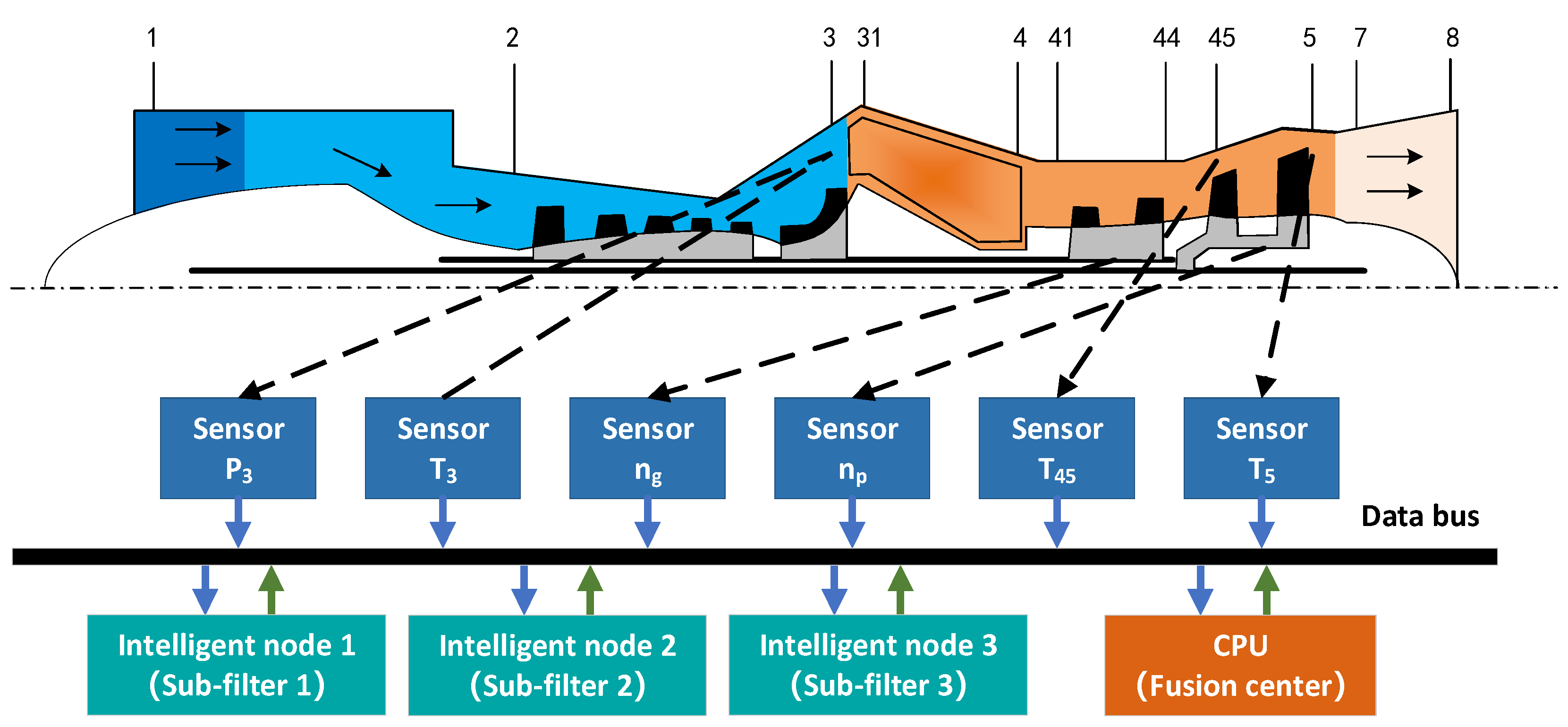
A turboshaft engine is taken as the studied plant in this paper, as shown in Figure 2, as well as the state monitoring structure under distributed architecture. Its main components include inlet, compressor, centrifugal compressor, combustor, gas turbine, power turbine, and nozzle. The component-level model of the studied turboshaft engine can be expressed by Equation (1), where the state vector includes the gas turbine rotor speed and power turbine rotor speed, the control parameters include fuel flow and collective pitch, and the output parameter , where the noise standard deviations used in the simulation are listed in Table 1. The implementation of sensor noise in our simulation involves the superposition of Gaussian-distributed random variables onto the sensor output signals. Table 1 explicitly documents the standard deviations associated with these random variables. The specific values of these standard deviations are determined with reference to [8]. Appropriate combinations of measurement parameters need to be selected from these six sensors for each sub-filter. The specific process will be introduced later.

Figure 2.
Distributed state monitoring architecture.

Table 1.
Available measurement instructions.
During an engine’s lifecycle, its components may experience faults and degradation. Health parameters are introduced to quantify the deviations between the ideal model and the actual engine. The health parameters are defined as the variation coefficients of the efficiency or flow capacity of the rotating components.
where subscript i = 1, 2, 3 indicates the compressor, gas turbine, and power turbine; and are the actual value of efficiency and flow capacity of the corresponding com-ponents under the current working condition; and and are the ideal values of the efficiency and flow capacity of the corresponding components under the fault-free condition.
Previous research has indicated that conventional Kalman Filters encounter significant challenges in distinguishing variations among gas turbine efficiency, power turbine efficiency, and power turbine flow capacity within turboshaft engines. This limitation is primarily attributed to the pronounced collinearity inherent in the measurement data when these three parameters undergo simultaneous changes. Therefore, this paper selects the health parameters as . After introducing the health parameters, the state parameters are augmented as . The Kalman Filter estimates the health parameters by analyzing the residuals between the actual engine measurements and the corresponding model outputs, thus realizing state monitoring.
When performing state estimation, the Kalman Filter typically requires that the number of measurements should be equal to or greater than the number of health parameters. However, the measured parameters may be collinear under different fault modes and simply adding more sensors does not necessarily improve estimation accuracy. In this study, the principles for selecting sensor groups for sub-filters are as follows: (1) Each sub-filter uses no fewer than five measurement parameters. (2) Each measurement group must include gas turbine and power turbine speed sensors. (3) The collinearity of measurement parameters should be minimized as much as possible for different failure modes. Given this, the similarity coefficient is used to evaluate the linear relationship of measurement parameters under different fault modes, and it is defined as follows:
where and are the measurement vectors under two different fault modes. The closer r is to 1, the stronger the collinearity between the two vectors, and vice versa. The health parameters are disturbed at the ground design point and the normalized measurement deviation is shown in Table 2. These errors represent the changes in measurements after a 2% step disturbance is applied to the health parameters under steady-state conditions of the turboshaft engine.
Table 2.
Measurement deviation after perturbating health parameters.
According to the above, four groups of measurement combinations are constructed, which are , , , and . Their similarities are calculated and listed in Table 3.
Table 3.
Similarity coefficient of measurement changes under health parameter step disturbances.
The data in Table 3 indicate a strong correlation for sensor group #2. This correlation is particularly pronounced when compressor efficiency and turbine efficiency decrease by −2%, resulting in a similarity of measurements reaching 0.9952, which is extremely close to 1. Such a high degree of similarity poses challenges for Kalman Filters in distinguishing between two failure modes. Consequently, sensor groups #1, #3, and #4 are selected for performance monitoring for the three sub-filters; the sensor measurement parameters used by each sub-filter are shown in Table 4. The symbol ‘√’ in the table denotes that the sensor is selected, whereas the symbol ‘—’ denotes that the sensor is not selected.
Table 4.
Sensor selection of sub-filters.
3.2. Adaptive Kalman Filtering Based on Measurement Reconstruction
For the cases of sensor data packet dropout, the independent distribution variable is used to describe the data receiving state, where i indicates the sensor number. When the measurement signals are normally received, ; otherwise, . Therefore, the signals received by the intelligent nodes can be expressed by Equation (10).
where is measurement of the N-th sensor used by the node at the last moment. The measurement equation of the system can be expressed as follows:
where .
If the engine is operating at a steady state, Equation (10) can be simplified as follows:
Once the system suffers the data packet dropout, the intelligent simulation nodes need to reconstruct the missing measurements. The residuals between actual measurements and model outputs are mainly affected by the modeling accuracy and noise when the engine runs in a steady state, i.e., . Under the premise that the modeling error is controllable, the weighted summed state vectors are calculated by a p-dimensional buffer to alleviate the effects of the noise.
where is the weight coefficient which satisfies and .
Therefore, the model outputs under the state are as follows:
To make the output closer to the actual situation, the model outputs are fused with the historical measurements:
where is the deviation between the last received measurements and the steady base point outputs before time k and is the weight factor.
This method expands the application range of the filter and makes the distributed control system have measurement reconstruction ability even when encountering continuous data packet dropout. Its principle and process are shown in Figure 3.
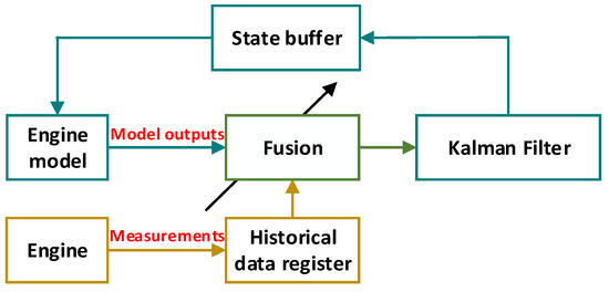
Figure 3.
Comprehensive measurement generation based on historical data and engine model.
Specially, according to this strategy, the comprehensive measurement at time k is ; thus, the measurement equation can be expressed as follows:
Substituting Equation (16) into Equation (5), we have the posterior state estimation equation.
The objective function is defined as follows:
where is the i-th element of ; thus, letting be the trace of the posterior error covariance matrix, Equation (18) can be rewritten as follows:
According to Equations (16) and (17), the posterior estimation error is as follows:
Let the measurement residual :
where ; substituting Equation (20) into Equation (21), we have the following:
Thus, the posterior error covariance matrix is rewritten as follows:
Since , , and are uncorrelated, Equation (23) can be simplified:
Combining Equation (24) with Equations (2) and (4), we have the following:
where is the covariance of the measurement error.
The principle of solving the optimal control law involves minimizing the cost function J. The Kalman gain matrix is obtained by solving .
In this regard, the adaptive Kalman update of each sub-filter in DAKF under comprehensive measurement information can be summarized, as in Algorithm 1.
| Algorithm 1: Sub-filter calculation in DAKF. |
| (1) Initialize state parameters; |
| according to Equation (5); |
| according to Equation (16) based on the data packet dropout; |
| ; (5) Update Kalman gain matrix and posterior error covariance matrix according to Equation (26); |
| and go to step (2). |
3.3. Signals’ Fusion Based on the Intelligent Buffer
The data may encounter packet dropout transmitting between the intelligent nodes and buses. Similarly to the measurement’s dropouts, let denote the receiving state of the local estimation result of the i-th sub-filter at time k. when the data are received normally; otherwise, .
A buffer of length L is set in the fusion center to store the local estimation results, with a weighting matrix as follows:
where is the weight coefficient matrix corresponding to the local estimation obtained by the i-th sub-filter at k-1 time (). Once data dropout occurs, the fused historical estimation that was restored in the buffer will replace the missing signals; thus, the local estimation update of the central processor can be expressed as follows:
The fusion equation based on the historical local estimation is as follows:
It should be pointed out that the weight coefficient matrix needs to be allocated according to the sequence of received data, the start of dropout, and the requirements of unbiased estimation. For this purpose, an L-dimensional vector is introduced:
Each element in the vector is assigned the weight according to the update time and satisfies the information conservation, i.e., .
To realize unbiased estimation, can be calculated as follows.
Letting , we can have . The covariance matrix of state estimation error between time k and m (k > m) is calculated as follows:
Thus, the error covariance matrix corresponding to the i-th buffer is as follows:
where , .
When there is no data dropout, the local estimation output by the sub-filter is still used. Therefore, the updated equation for the integrated local error covariance matrix in the central control node is as follows.
Performing global fusion of the local fusion estimation results and the local fusion error covariance matrices obtained from different sub-filters, we have
where is the adjustment coefficient, which satisfies .
The information distribution process is as follows:
When the dropout rate is high, the buffer may be unable to be updated for multiple consecutive cycles, and the estimation results of the corresponding sub-filter may be temporarily shielded. Therefore, the calculation process of the fusion algorithm based on the state buffer at the fusion center can be obtained, as shown in Algorithm 2.
| Algorithm 2: State buffer-based fusion. |
| (1) Initialize state variables and error covariance matrix; |
| (2) Receive the local state estimation results from the sub-filters via the bus and check for data dropout: If the dropout occurs |
| Fuse the local estimation results in the corresponding buffer of the filter to obtain the local estimation results at this time step; Else Store the sub-filter local estimation results into the state buffer; End |
| (3) Perform global fusion and allocation of the integrated local estimation results and integrated local error covariance matrices obtained from different sub-filters, and upload the allocation results to the data bus; |
| , return to step 2 until the simulation ends. |
As the buffer length L increases, the performance monitoring accuracy improves, but this also leads to an increase in the computation time. Assuming the dropout rate from the intelligent simulation node to the bus is 20%, the engine path components are injected some deviation as fault mode 6, Table 5 shows the computation time at the central control node and the fault estimation root mean square errors (RMSE) under different buffer lengths. RMSE serves as a crucial metric for evaluating the filtering accuracy of our algorithm across different samples and conditions. The RMSE is calculated using the following formula:
where represents the total number of simulation steps, denotes the state estimate from our engine filter at step k, indicates the true state of the engine at step k.
Table 5.
Fusion Performance under different buffer lengths.
As shown in Table 5, with the increase in L, the additional computation time-consuming required by the central control node per cycle increases; meanwhile, the RMSE decreases. Therefore, in this study, a buffer length of 5 is chosen as a compromise.
3.4. Data Packet Dropout Coping Strategies
When data packet loss occurs between the central control node and the intelligent simulation node, the intelligent simulation node will default to using the global filtering result from the central control node received during the previous step as the prior estimate for the current simulation step. Due to the fault tolerance capability inherent in the distributed control architecture, the local estimation results of the sub-filters already possess a certain level of accuracy. Therefore, the local filtering result from the previous step can be used as the prior estimate for the next step. The calculation process for the prior estimate at the intelligent simulation node is shown in Algorithm 3.
| Algorithm 3: State buffer-based fusion. |
| (1) Initialize the prior estimate; |
| (2) Determine whether data dropout has occurred between the central control node and the intelligent simulation node: If the dropout occurs and from the previous step to calculate the prior estimate; Else received from the bus to calculate the prior estimate; End |
| (3) Perform local state estimation as in Algorithm 2; |
| ; return to step 2 until the simulation ends. |
4. Construction of Distributed Control Simulation Platform
4.1. TTP/C Communication Scheduling
The time-triggered protocol/C (TTP/C) is a typical time-triggered communication protocol on which the distributed control architecture physical platform is based, and it has advantages in terms of real-time performance, redundancy design, fault-tolerant capability, and reconfigurability. Therefore, it provides a reliable underlying communication solution for aircraft engines.
A. Interface module
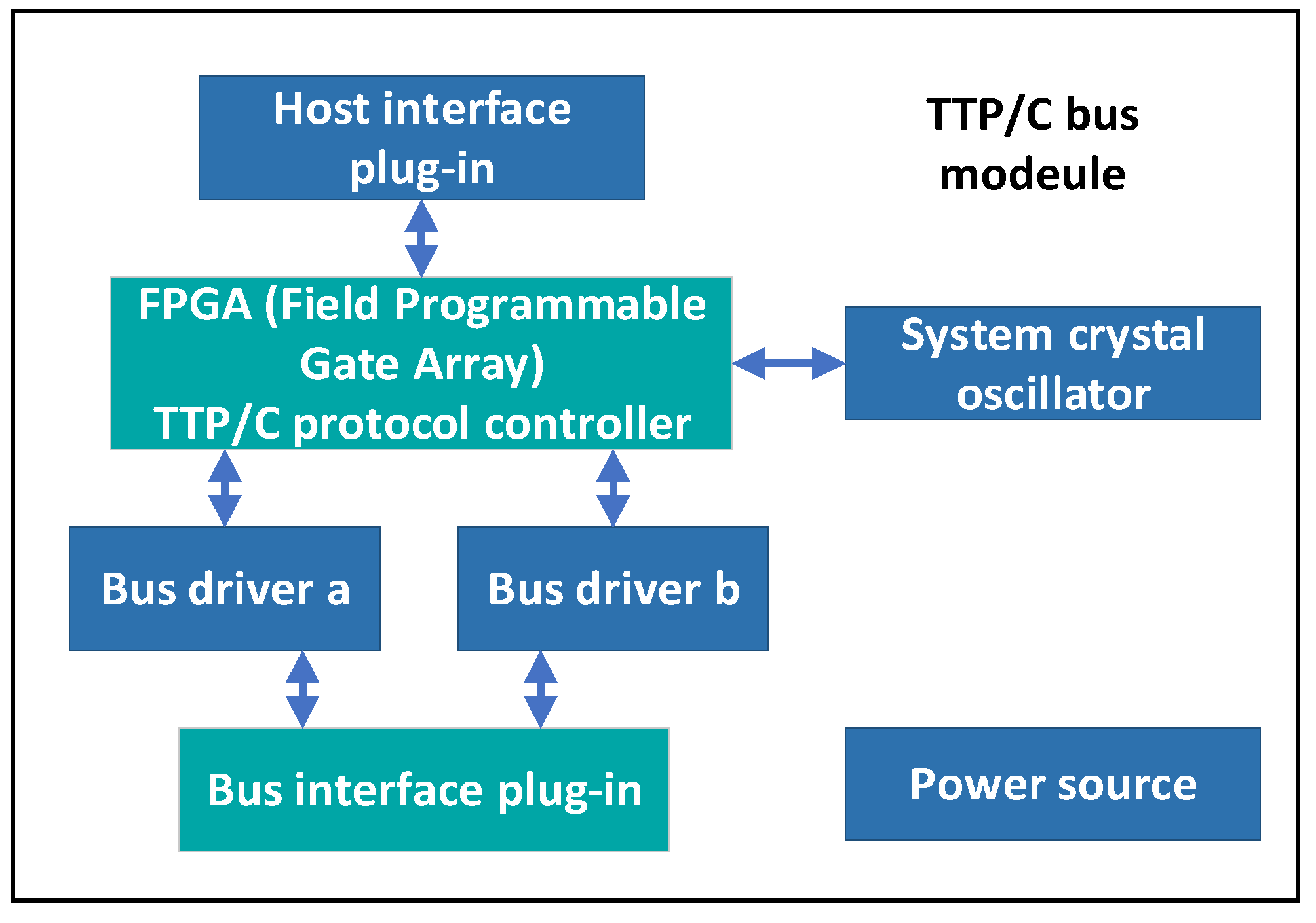
The bus access functionality of TTP/C is provided by the interface module, where the main function is to send the host interface data while also receiving the designated data from other nodes according to the specified time schedule. As shown in Figure 4, the bus structure primarily consists of the power supply, bus interface plug-in, driver, protocol controller, host interface plug-in, and system oscillator. To design the cluster scheduling plan, we should identify each node on the TTP/C bus first, and then generate the cluster scheduling plan into a message descriptor list (MEDL) table file, which is finally downloaded to the bus controller.

Figure 4.
TTP/C bus structure.
B. Cluster design based on TTP/C
Step 1: Set cluster parameters. Since the sampling period of the aircraft engine is 20 ms, the length of each timing division multiple access (TDMA) round is also set to 20 ms. Other parameters are shown in Table 6.
Table 6.
Cluster planning and design parameters.
Step 2: Design host parameters. The distributed control architecture includes three intelligent simulation nodes, and the parameters to be defined for each node are shown in Table 7.
Table 7.
Parameter definitions of intelligent simulation nodes.
Step 3: Use the TTP_Build toolset to generate the MEDL table program. Compile the cluster database designed in the previous step to obtain the cluster information.
Step 4: Use TTP_Load to download the configured MEDL table program. Load the serial configuration file into the TTP_Load tool until the table program deployment is completed.
4.2. Hardware Platform Construction
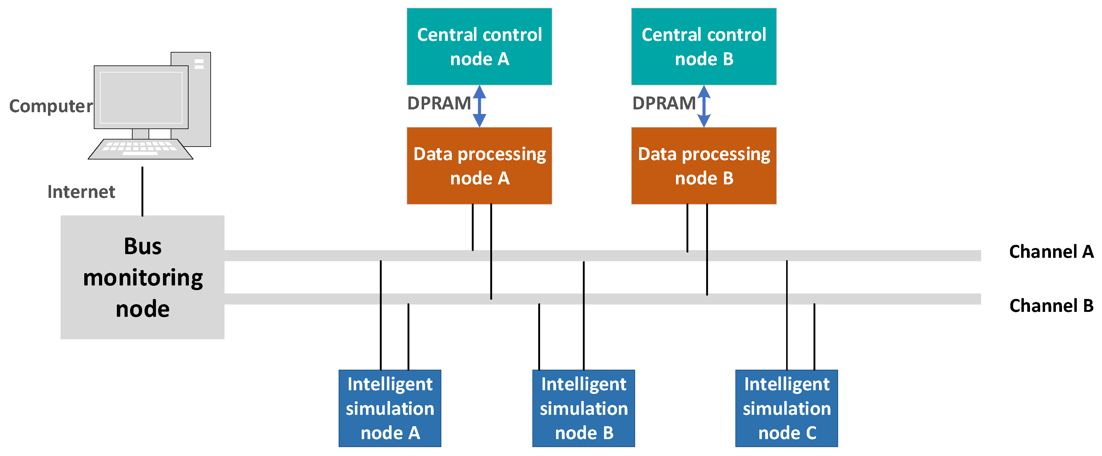
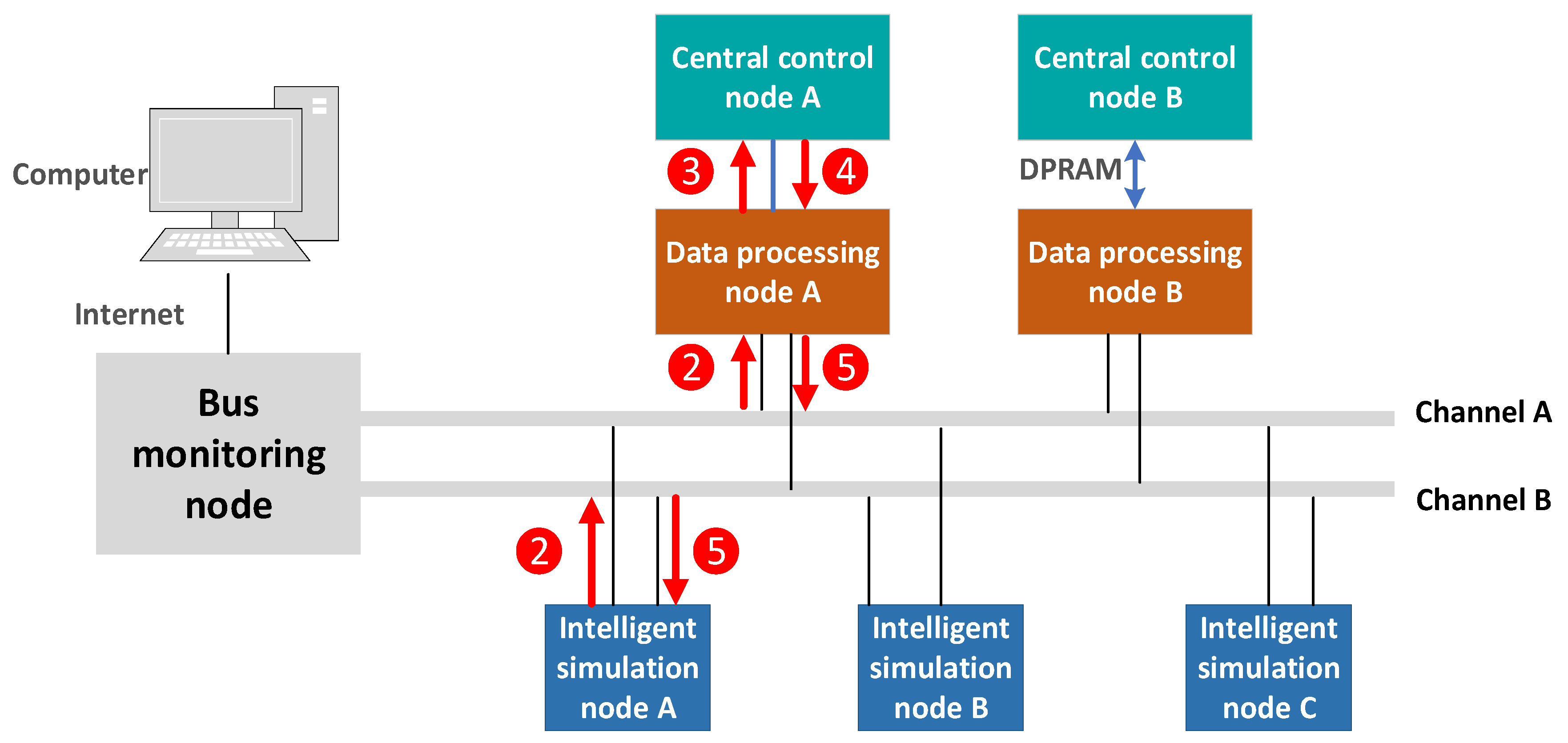
The hardware simulation platform mainly consists of power supply, host computer, intelligent simulation nodes, bus monitoring nodes, data processing nodes, a central control node, and data bus. The composition of the distributed control architecture hardware simulation platform is shown in Figure 5.
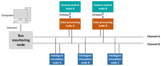
Figure 5.
Distributed control architecture.
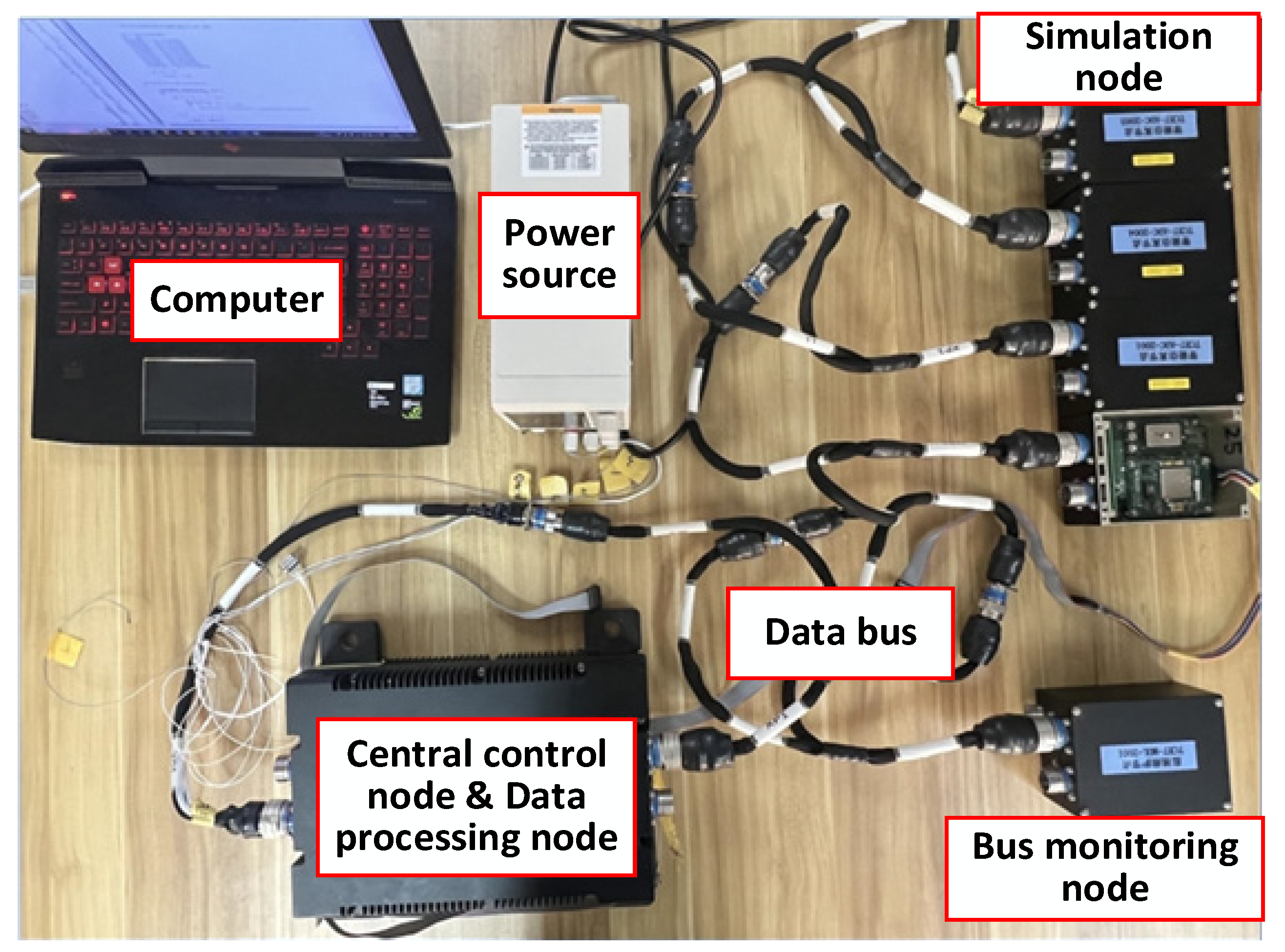
Figure 6 shows the physical platform of the distributed control architecture built. In the figure, the upper right corner represents the intelligent simulation nodes, the lower right corner represents the bus monitoring node, and the lower left corner shows the two central control nodes and two data processing nodes, which are enclosed.

Figure 6.
Physical set-up of distributed control architecture.
The distributed control system illustrated in Figure 6 primarily consists of a supervisory computer, a central control and data processing node, a simulation node, a bus monitoring node, and a power supply. Their respective functions are as follows: The central control node is utilized to simulate the mathematical model of the engine. The supervisory computer deploys the engine model to the controller through developed software. It establishes an independent data transmission bus with the data processing node, enabling data interaction between the engine simulator and the data processing node. The data processing node is primarily responsible for reading from and writing to the bus, facilitating data transmission with the control node. The intelligent simulation node is designed for algorithm computation. The bus monitoring node is tasked with monitoring the data flow on the TTP/C bus and transmitting it to the PC via network communication, thereby enabling the monitoring of data sent by each node. The supervisory computer is mainly used for data analysis, control scheduling, and human–machine interaction, while the power supply provides electricity to all modules. Table 8 lists the specific parameters of each node, and their workflow is described as follows.
Table 8.
Distributed control architecture hardware parameters.
- (a)
- Central control nodes: Each central control node is equipped with a P2020 processor with a main frequency of 800 MIPS (millions of instructions per second), providing strong computational capability. The P2020 chip is produced by Freescale (now part of NXP Semiconductors, headquartered in Eindhoven, The Netherlands). To enable data exchange, the central control nodes use dual-ported random-access memory (DPRAM) and establish the independent data transmission bus to communicate with the data processing nodes. The DPRAM has dedicated read/write addresses, and in this study, the read/write address range of the DPRAM is defined as 0×0000-0×1FFE (hexadecimal expression).
- (b)
- Intelligent simulation nodes: Each intelligent simulation node is equipped with an MPC5566 processor, with a main frequency of 132 MIPS. TTP/C driver chips are used in the intelligent simulation nodes to facilitate communication with the data bus.
- (c)
- Data processing node: Each data processing node is equipped with an MPC5674 processor (manufactured by NXP Semiconductors), with a main frequency of 264 MIPS. Like intelligent simulation nodes, the data processing nodes also use TTP/C driver chips to enable communication with the data bus.
- (d)
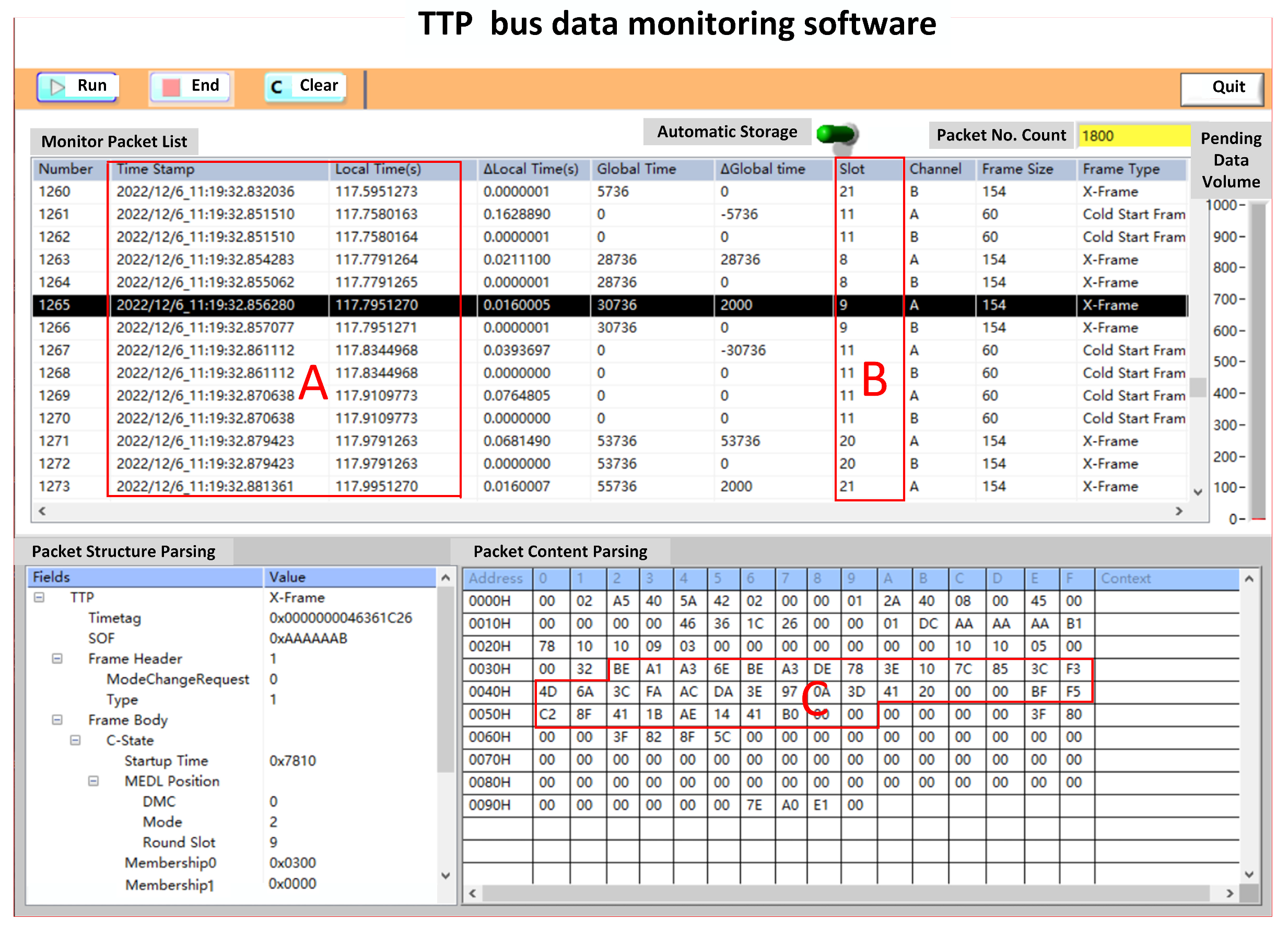
- Bus monitoring node: The data on the data bus can be read by the bus monitoring node and sent to the host computer for data collection by signal acquisition software. The data monitoring interface is shown in Figure 7. It consists of several parts:
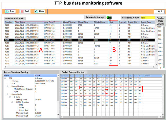 Figure 7. Data monitoring interface.
- Area A displays the time at which each node sends data to the bus.
- Area B shows the node information of the data sender at that moment.
- Area C shows the specific data sent by the node to the bus.
Data are transmitted on the bus in byte format. After each node receives the data, it converts it into floating-point format for further use. Once the calculation is completed, the required data are converted back into byte format and transmitted back to the data bus. Summarizing the workflow of each node, the overall workflow of the distributed control architecture is shown in Figure 8.
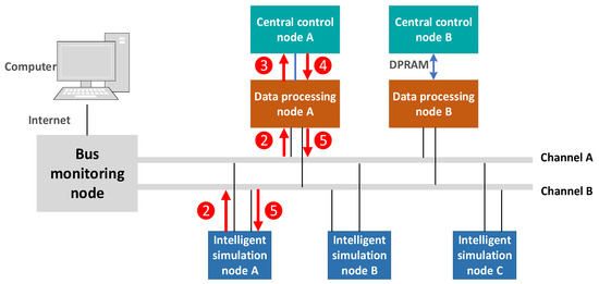
Figure 8.
Communication flow of the distributed control architecture.
5. Test and Analysis
5.1. Full Digital Simulation
A. Validation of distributed performance monitoring method under network uncertainty
To verify the proposed distributed performance monitoring method, we conduct some simulations at several representative operating points of the turboshaft engine, including the design point at ground level (H = 0 m, Ma = 0) and off-design points at H = 2000 m and Ma = 0.1. The typical gas path component faults of a turboshaft engine and the corresponding health parameter deviations are listed in Table 9. The engine dynamics are represented by a high-accuracy mathematical model established in [40].
Table 9.
Typical failure modes of a turboshaft engine.
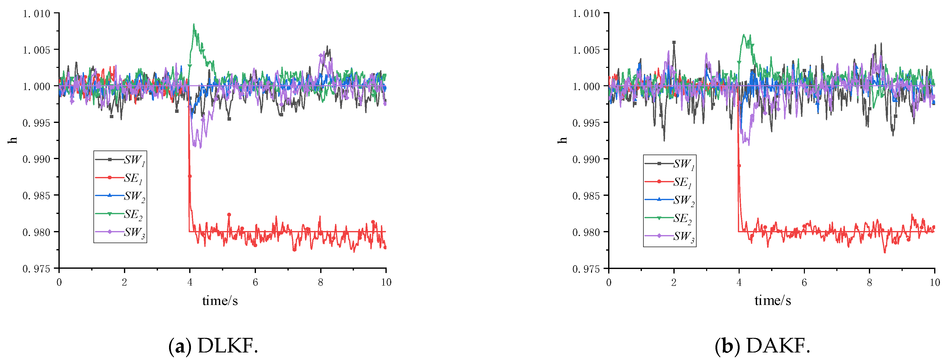
In practical applications, the data dropout rate may vary across different missions. For simplicity’s sake, we assume that the dropout rate stays unchanged across all stages in this study. As mentioned earlier, when no dropout occurs, the DAKF is consistent with the Distributed Linear Kalman Filter (DLKF). The comparison between DLKF and DAKF with a dropout loss rate of 0 is shown in Figure 9, under failure mode 2 in Table 9. As can be seen from the results, when the packet loss rate is 0, the simulation results of the DLKF and DAKF methods are nearly indistinguishable, with the RMSE of the DLKF being 0.0085 and that of the DAKF being 0.0084.
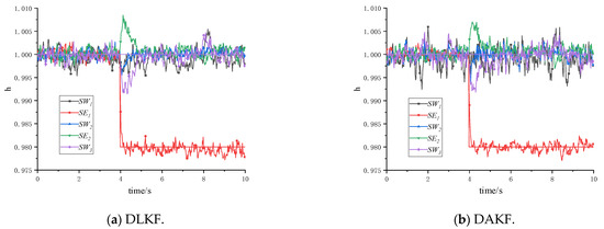
Figure 9.
Performance monitoring results of DLKF and DAKF when the dropout rate is 0.
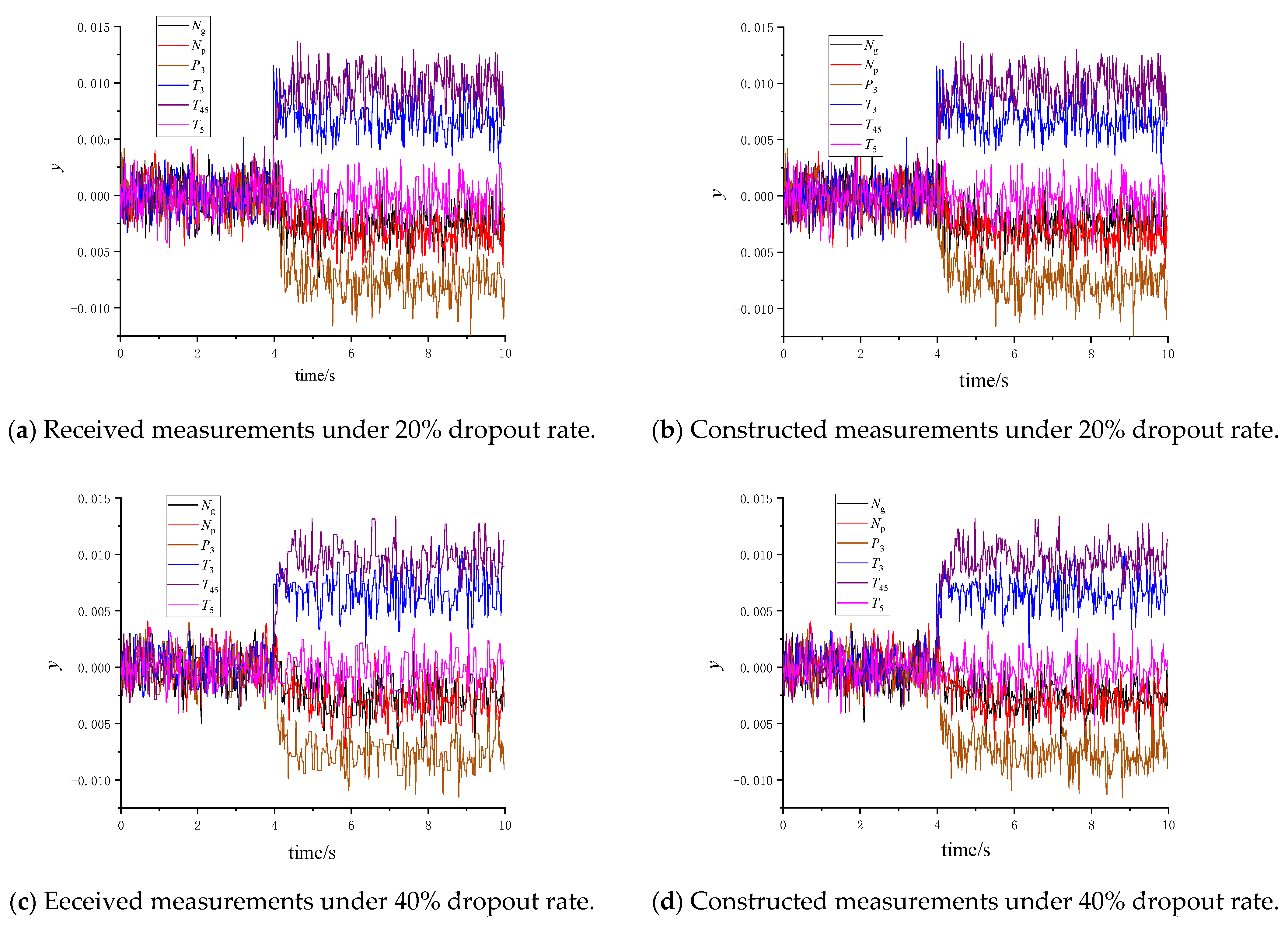
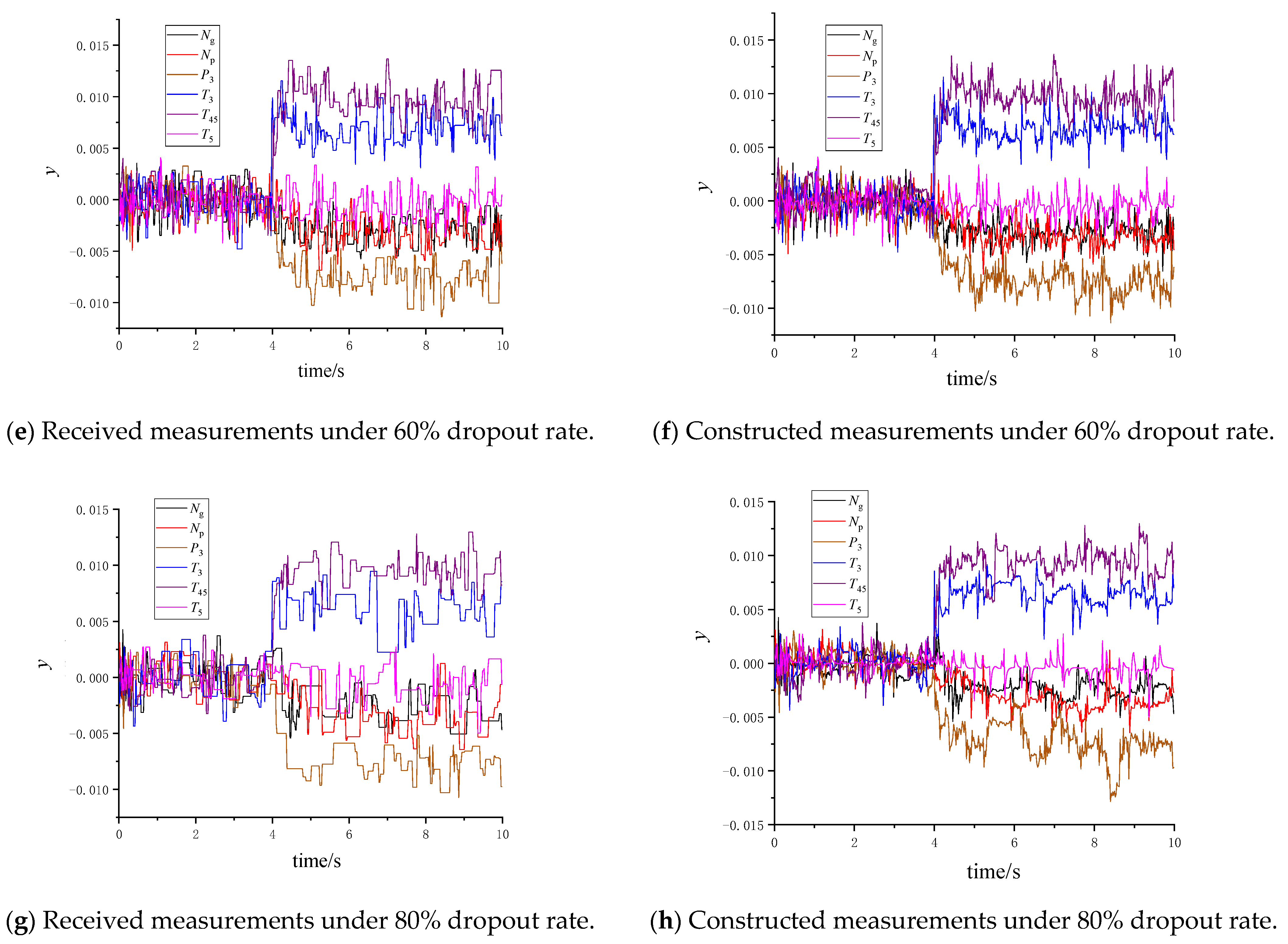
However, when different dropout rates are introduced, the DAKF method would combine the historical measurements with the engine’s mathematical model to reduce the influence of the dropout. Figure 10 presents the measured parameters received by the distributed control system and the constructed measurements under different dropout rates (20%, 40%, 60%, and 80%).

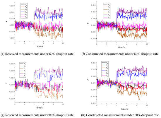
Figure 10.
Measurement data received by distributed control system under different dropout rates.
Figure 10a,c,e,g show the sensor data received by the distributed control system under different packet loss rates. It can be observed that some of the data points in the figures are not updated due to packet loss, resulting in shapes parallel to the x-axis. As the packet loss rate increases, this phenomenon becomes more pronounced. Figure 10b,d,f,h present the composite measurement data, which are composed of the received measurement data and the reconstructed measurement data for the lost packets. These variations in signal quality effectively demonstrate how our method performs across different network reliability scenarios, highlighting its robustness in handling packet dropout during data transmission.
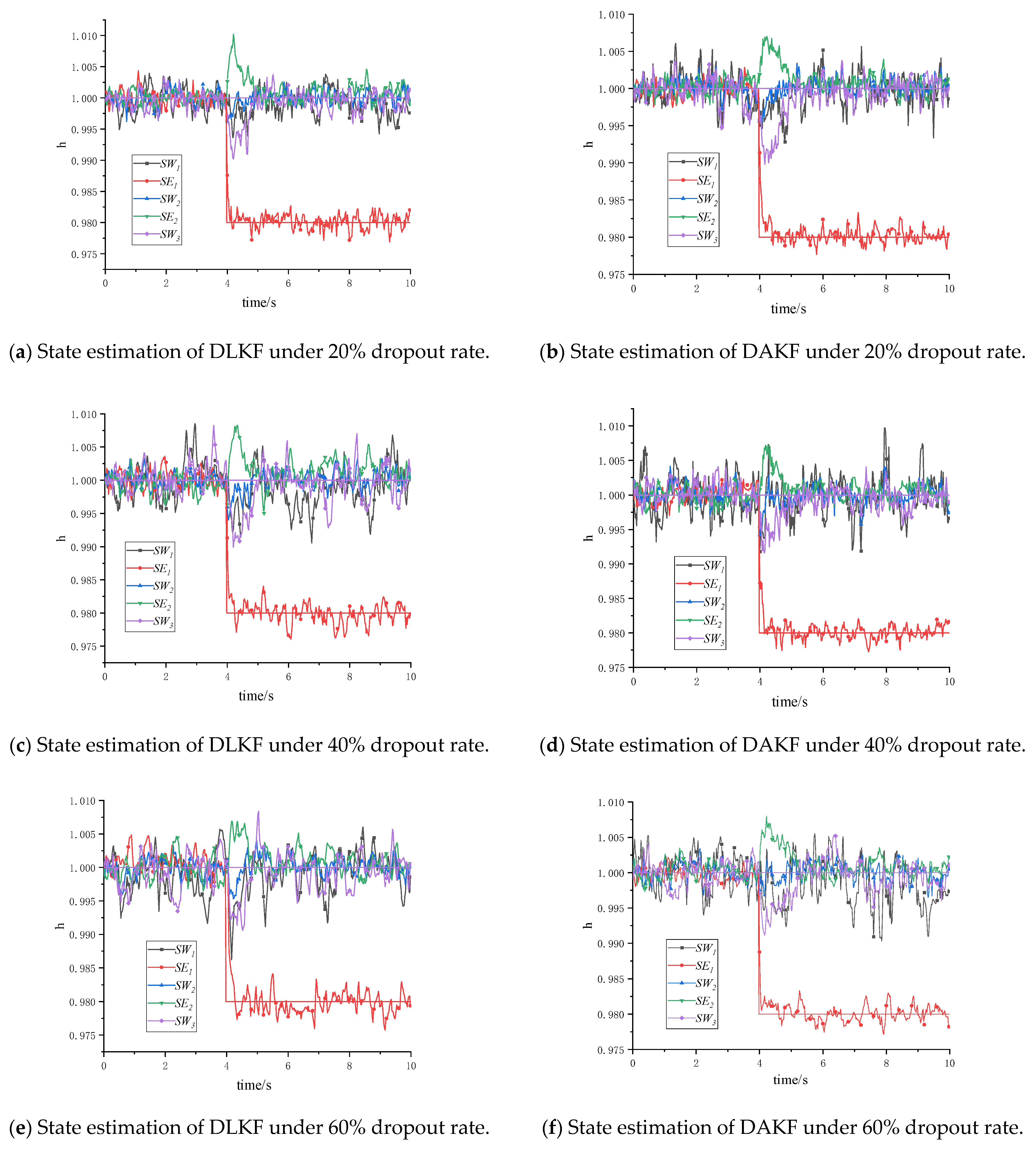
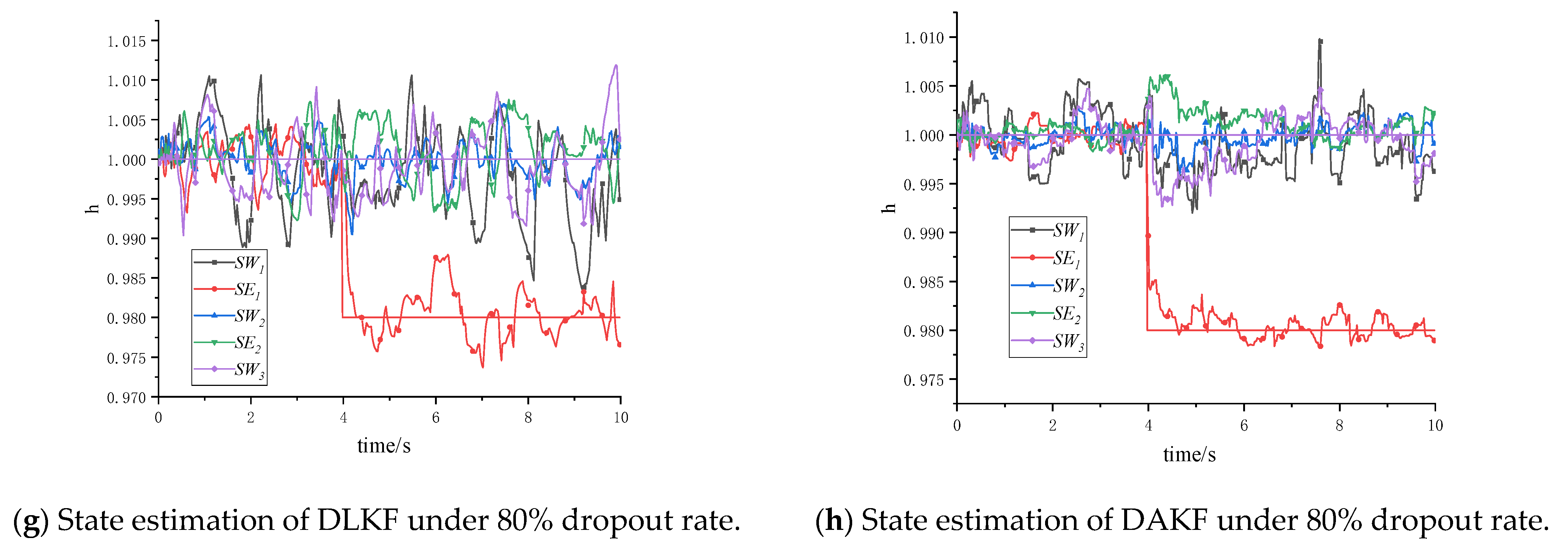
Further comparison of the state estimation accuracy between the DLKF and DAKF methods under different packet loss rates is shown in Figure 11, which illustrates the state estimation performance of both methods under varying packet loss conditions. In addition, Figure 12 presents the estimation RMSEs of the DLKF and DAKF under different dropout rates.
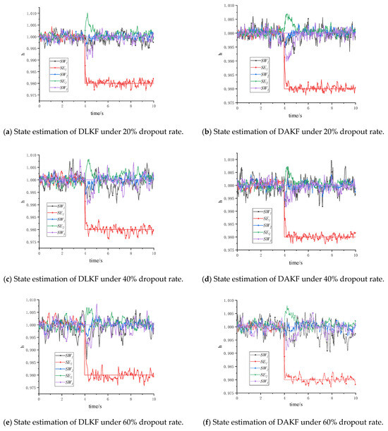
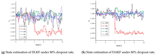
Figure 11.
State estimation results of DLKF and DAKF under different dropout rates.
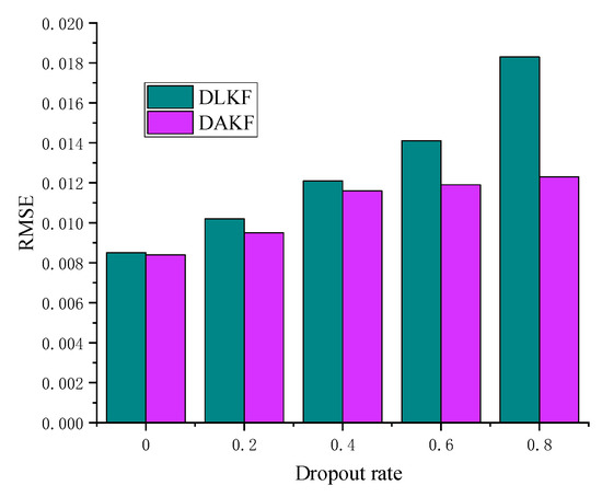
Figure 12.
Estimation RMSEs under different dropout rates.
From Figure 11 and Figure 12, it can be seen that when the dropout rate is low, both DLKF and DAKF can provide good estimation results. However, as the dropout rate increases, the DLKF method gradually exhibits a trend to converge, whereas the DAKF method shows better robustness. However, once the dropout rate reaches a threshold, the decline in accuracy for the DAKF method slows down significantly. The higher the dropout rate, the more pronounced the accuracy advantage of the DAKF method becomes.
Based on the above simulations, it can be concluded that the DAKF method designed in this paper effectively mitigates the performance monitoring accuracy degradation caused by the uncertainties in the distributed architecture network, especially under a high dropout rate.
5.2. Experimental Verification Under Distributed Architecture
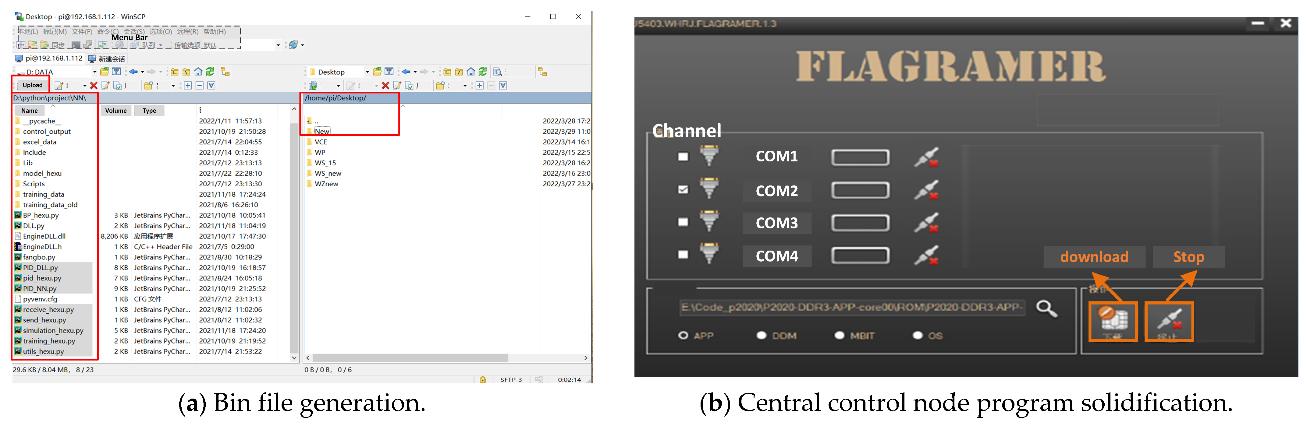
In this section, we deploy the proposed algorithm onto a physical platform based on a distributed control architecture. There are two central control nodes: One’s purpose is to host the fusion center, receiving and integrating the local filtering results from the sub-filters and transmitting the fused results to the data bus. The other one’s purpose is to generate sensor data and transmit it to the data bus. The development software platform used for the central control node is CodeWarrior 5.7.0. Figure 13 illustrates the operational flow for deploying the central control node program.
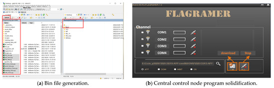
Figure 13.
The solidification process of the central control node program.
The intelligent simulation nodes deploy the sub-filters. These nodes host the engine mathematical model and read sensor data from the data bus, as well as global estimation results from the central control node, to compute the local filtering results for the sub-filters. The development software platform used for the intelligent simulation nodes is CodeWarrior 5.9.0. The performance monitoring algorithm program is compiled using CodeWarrior 5.9.0 and the file is deployed to the intelligent simulation nodes using the programming tool FlaGramer (a specialized software tool used for firmware burning into hardware platforms, which usually operates with specific hardware systems).
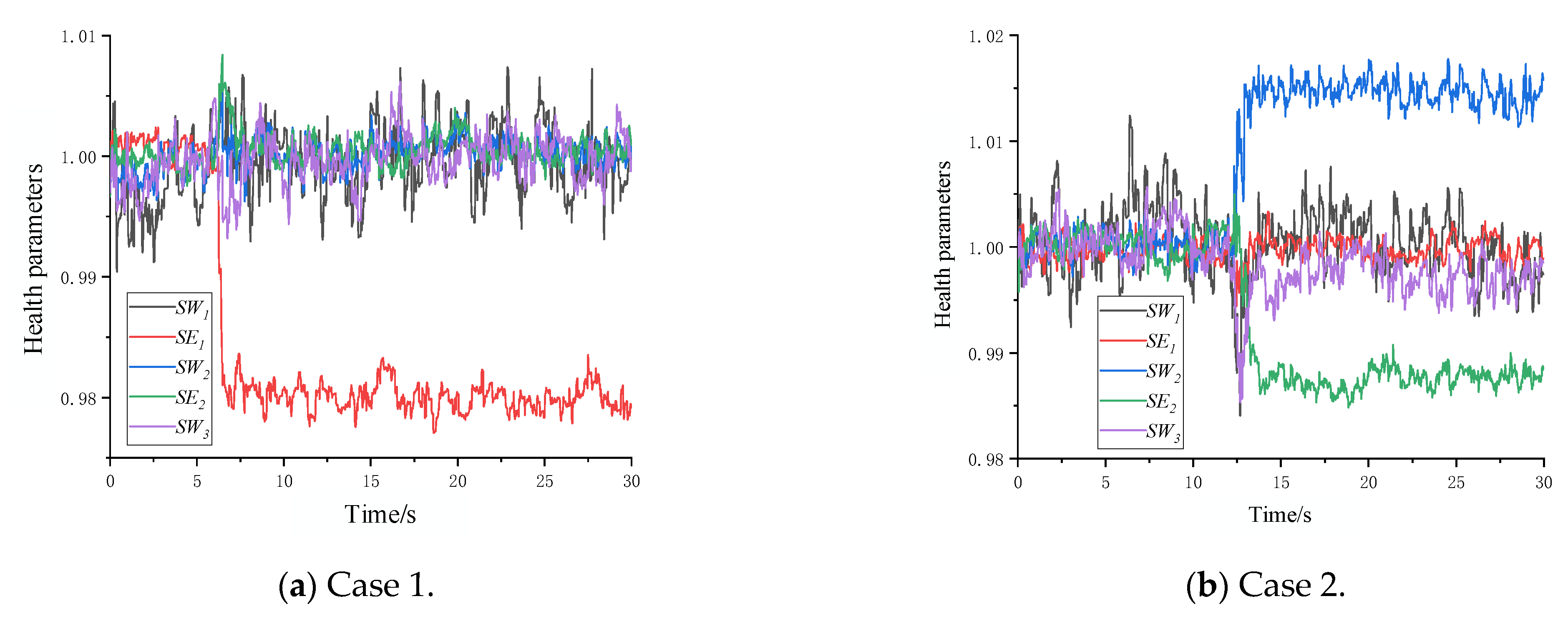
To validate the estimation performance of the proposed DAKF, further simulation verification is conducted under the network uncertainty within the distributed control architecture. The simulation is carried out at the operating point H = 0 m, Ma = 0, with a bus dropout rate of 30%. The fault modes correspond to failure mode 6 (case 1) and failure mode 4 (case 2) listed in Table 9. Since the distributed control architecture does not provide functionality for simulating network failure environments, the data dropout is modeled as a random process which follows a Bernoulli distribution. The performance monitoring results under network uncertainty in the distributed control architecture are shown in Figure 14.
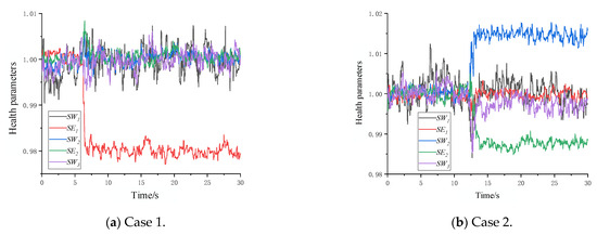
Figure 14.
DAKF verification under network uncertainty of distributed control architecture.
Figure 14 shows the superiority of the DAKF designed in this paper. In Figure 14a, it can be seen that around 6 s, there is a significant decline in the compressor flow coefficient, indicating a fault in the compressor. In Figure 14b, it is evident that around 12 s into the simulation, both the gas turbine flow and efficiency coefficients experience an abrupt change, allowing for the conclusion that a fault has occurred in the gas turbine at that moment. The results show that the distributed performance monitoring method can effectively monitor the engine performance and has sufficient fault tolerance ability.
6. Conclusions
Aero-engine performance monitoring plays a significant role in engine health management. Concurrently, the distributed control architecture exhibits prominent potential for future development. This paper investigates a distributed performance monitoring method for turboshaft engines. Specifically, we designed a Kalman Filter suitable for distributed systems and an adaptive improvement strategy along with a state buffer to address the issue of data packet loss, thereby maintaining state estimation performance under network uncertainties. Simulation results on all digital and HIL platforms demonstrate that the proposed DAKF method exhibits strong robustness under various levels of packet loss rates. The RMSE of health parameter estimation does not exceed 0.012, compared to 0.019 for the DLKF method used as a control, effectively mitigating the decline in performance monitoring accuracy caused by uncertainties in the distributed architecture network.
This paper improves the distributed filtering algorithm and proposes a novel adaptive strategy, which can be extended to various types of aero engines, such as turbofan and variable-cycle engines. There are several opportunities for further exploration. For instance, this work only considers the impact of data packet loss, but data delay is also a typical manifestation of network uncertainty. Further refining the state buffer strategy of this method to accommodate scenarios where both data delay and packet loss coexist would be of significant interest. In conclusion, these efforts hold practical value and inspire future research and development. By continuing to explore these avenues, we can anticipate more significant advancements and practical applications in this field.
Nomenclature List
| Nomenclature | |
| DAKF | Distributed Adaptive Kalman Filter |
| DEKF | Distributed Extended Kalman Filter |
| DLKF | Distributed Linear Kalman Filter |
| DPRAM | Dual-ported random-access memory |
| EHM | Engine health management |
| EKF | Extended Kalman Filter |
| H | Altitude |
| KCF | Kalman Consensus Filter |
| Ma | Mach number |
| MEDL | Message Description List |
| MIPS | Millions of instructions per second |
| RMSE | Root mean square error |
| SUKF | Spherical Unscented Kalman Filter |
| TDMA | Timing division multiple access |
| TTP/C | Time-triggered protocol/category C |
| Subscripts | |
| d | Design point |
| f | Fuel |
| g | Gas turbine |
| p | Power turbine |
| 3 | Compressor exit |
| 45 | Power turbine inlet |
| 5 | Power turbine exit |
| 8 | nozzle exit |
Author Contributions
Methodology, C.W. and X.Z. (Xinyu Zhu); Formal analysis, J.H.; Writing—original draft, X.Z. (Xin Zhou); Writing—review & editing, F.L. All authors have read and agreed to the published version of the manuscript.
Funding
This research received no external funding.
Data Availability Statement
The original contributions presented in this study are included in the article. Further inquiries can be directed to the corresponding author.
Conflicts of Interest
There is no conflict of interest with respect to the research, authorship, and/or publication of this article.
References
- Tegtmeier, L.A. 10-year global MRO forecast. Overhaul Maint. 2011, 17, 28–31. [Google Scholar]
- Amare, F.D.; Gilani, S.I.; Aklilu, B.T.; Mojahid, A. Two-shaft stationary gas turbine engine gas path diagnostics using fuzzy logic. J. Mech. Sci. Technol. 2017, 31, 5593–5602. [Google Scholar] [CrossRef]
- Li, Y.G.; Korakiantis, T. Nonlinear Weighted-Least-Squares Estimation Approach for Gas-Turbine Diagnostic Applications. J. Propuls. Power 2012, 27, 337–345. [Google Scholar] [CrossRef]
- Lee, S.-M.; Choi, W.-J.; Roh, T.-S.; Choi, D.-W. A study on separate learning algorithm using support vector machine for defect diagnostics of gas turbine engine. J. Mech. Sci. Technol. 2008, 22, 2489–2497. [Google Scholar] [CrossRef]
- Depold, H.R.; Gass, F.D. The application of expert systems and neural networks to gas turbine prognostics and diagnostics. J. Eng. Gas Turbines Power-Trans. ASME 1999, 121, 607–612. [Google Scholar] [CrossRef]
- Zhao, N.; Wen, X.; Li, S. A review on gas turbine anomaly detection for implementing health management. Turbo Expo Power Land Sea Air 2016, 49682, V001T22A009. [Google Scholar]
- Tolani, D.; Yasar, M.; Chin, S.; Ray, A. Anomaly detection for health management of aircraft gas turbine engines. In Proceedings of the 2005, American Control Conference, Portland, OR, USA, 8–10 June 2005. [Google Scholar]
- Lu, F.; Jin, P.; Huang, J.; Wang, C.; Qin, H. Aircraft engine hot-section virtual sensor creation and gas path performance monitoring. Proc. Inst. Mech. Eng. Part G J. Aerosp. Eng. 2022, 236, 879–899. [Google Scholar] [CrossRef]
- Zhou, H.; Huang, J.; Lu, F. Reduced kernel recursive least squares algorithm for aero-engine degradation prediction. Mech. Syst. Signal Process. 2017, 95, 446–467. [Google Scholar] [CrossRef]
- Chen, Q.; Sheng, H.; Zhang, T. An improved nonlinear onboard adaptive model for aero-engine performance control. Chin. J. Aeronaut. 2023, 36, 317–334. [Google Scholar] [CrossRef]
- Liu, X.; Zhu, J.; Luo, C.; Xiong, L.; Pan, Q. Aero-engine health degradation estimation based on an underdetermined extended Kalman filter and convergence proof. ISA Trans. 2022, 125, 528–538. [Google Scholar] [CrossRef]
- Wang, P.; Cheng, N.; Li, Q. The estimation algorithm for component health parameter of turbofan engine. In Proceedings of the 2016 IEEE Chinese Guidance, Navigation and Control Conference (CGNCC), Nanjing, China, 12–14 August 2016; pp. 75–80. [Google Scholar] [CrossRef]
- Chen, C.; Zheng, Q.; Zhang, H. Research on selection method of aero-engine health parameters based on correlation and condition number. Proc. Inst. Mech. Eng. Part G J. Aerosp. Eng. 2023, 237, 2939–2951. [Google Scholar] [CrossRef]
- Liu, B.; Ma, Y.; Wu, Y.; Sun, X. An improved Kalman filter based on neural network for turbofan engine gas-path health estimation. In Proceedings of the 2020 39th Chinese Control Conference (CCC), Shenyang, China, 27–29 July 2020; pp. 4135–4140. [Google Scholar] [CrossRef]
- Zhao, Y.-P.; Jin, H.-J.; Liu, H. Gas Path Fault Diagnosis of Turboshaft Engine Based on Novel Transfer Learning Methods. J. Dyn. Sys. Meas. Control 2024, 146, 031010. [Google Scholar] [CrossRef]
- Yu, Y.; Wang, Y.; Zhang, G.; Wang, J. Research of Fault Feature Extraction and Analysis Method Based on Aeroengine Fault Data. In Proceedings of the 2020 Chinese Automation Congress (CAC), Shanghai, China, 6–8 November 2020; pp. 2960–2965. [Google Scholar] [CrossRef]
- Willsky, A.S.; Bello, M.; Castanon, D.A.; Levy, B.C.; Verghese, G. Combining and updating of local estimates and regional maps along sets of one-dimensional tracks. IEEE Trans. Autom. Control 1982, 27, 799–813. [Google Scholar] [CrossRef]
- Carlson, N.A. Federated square root filter for decentralized parallel processors. IEEE Trans. Aerosp. Electron. Syst. 1990, 26, 517–525. [Google Scholar] [CrossRef]
- Ribeiro, A.; Giannakis, G.B.; Roumeliotis, S.I. SOI-KF: Distributed Kalman filtering with low-cost communications using the sign of innovations. IEEE Trans. Signal Process. 2006, 54, 4782–4795. [Google Scholar] [CrossRef]
- Chen, B.; Zhang, W.A.; Yu, L. Distributed finite-horizon fusion Kalman filtering for bandwidth and energy constrained wireless sensor networks. IEEE Trans. Signal Process. 2014, 62, 797–812. [Google Scholar] [CrossRef]
- Safari, S.; Shabani, F.; Simon, D. Multirate multisensor data fusion for linear systems using Kalman filters and a neural network. Aerosp. Sci. Technol. 2014, 39, 465–471. [Google Scholar] [CrossRef]
- Mahmoud, M.S.; Emzir, M.F. State estimation with asynchronous multi-rate multi-smart sensors. Inf. Sci. 2012, 196, 15–27. [Google Scholar] [CrossRef]
- Liu, L.; Yang, A.; Tu, X.; Fei, M.; Naeem, W. Distributed weighted fusion estimation for uncertain networked systems with transmission time-delay and cross-correlated noises. Neurocomputing 2017, 270, 54–65. [Google Scholar] [CrossRef]
- Olfati-Saber, R. Distributed Kalman filtering for sensor networks. In Proceedings of the 46th IEEE Conference on Decision and Control, New Orleans, LA, USA, 12–14 December 2007. [Google Scholar]
- Olfati-Saber, R. Kalman-consensus filter: Optimality, stability, and performance. In Proceedings of the Joint 48th IEEE Conference on Decision and Control (CDC)/28th Chinese Control Conference (CCC), Shanghai, China, 16–18 December 2009. [Google Scholar]
- Kamal, A.T.; Ding, C.; Song, B.; Farrell, J.A.; Roy-Chowdhury, A.K. A generalized Kalman consensus filter for wide-area video networks. Proccedings of the 50th IEEE Conference of Decision and Control (CDC)/European Control Conference (ECC), Orlando, FL, USA, 12–15 December 2011. [Google Scholar]
- Xiong, J.; Lam, J. Stabilization of linear systems over networks with bounded packet loss. Automatica 2007, 43, 80–87. [Google Scholar] [CrossRef]
- Xie, L.; Xie, L. Peak covariance stability of a random Riccati equation arising from Kalman filtering with observation losses. J. Syst. Sci. Complex. 2007, 20, 262–272. [Google Scholar] [CrossRef]
- Huang, M.; Dey, S. Stability of Kalman filtering with Markovian packet losses. Automatica 2007, 43, 598–607. [Google Scholar] [CrossRef]
- Qian, H.; Qiu, Z.; Wu, Y. Robust extended Kalman filtering for nonlinear stochastic systems with random sensor delays, packet dropouts and correlated noises. Aerosp. Sci. Technol. 2017, 66, 249–261. [Google Scholar] [CrossRef]
- Wang, X.; Liu, W.; Deng, Z. Robust weighted fusion Kalman estimators for systems with multiplicative noises, missing measurements and uncertain-variance linearly correlated white noises. Aerosp. Sci. Technol. 2017, 68, 331–344. [Google Scholar] [CrossRef]
- Rezaei, H.; Esfanjani, R.M.; Sedaaghi, M.H. Improved robust finite-horizon Kalman filtering for uncertain networked time-varying systems. Inf. Sci. 2015, 293, 263–274. [Google Scholar] [CrossRef]
- Schenato, L. Optimal estimation in networked control systems subject to random delay and packet drop. IEEE Trans. Autom. Control. 2008, 53, 1311–1317. [Google Scholar] [CrossRef]
- Rezaei, H.; Mahboobi Esfanjani, R.; Farsi, M. Robust filtering for uncertain networked systems with randomly delayed and lost measurements. IET Signal Process. 2015, 9, 320–327. [Google Scholar] [CrossRef]
- Nikfetrat, A.; Esfanjani, R.M. Adaptive Kalman filtering for systems subject to randomly delayed and lost measurements. Circuits Syst. Signal Process. 2018, 37, 2433–2449. [Google Scholar] [CrossRef]
- Shi, L.; Xie, L.; Murray, R.M. Kalman filtering over a packet-delaying network: A probabilistic approach. Automatica 2009, 45, 2134–2140. [Google Scholar] [CrossRef]
- Zhu, C.; Xia, Y.; Yan, L.; Fu, M. Centralized fusion over unreliable networks. Int. J. Control. 2012, 85, 409–418. [Google Scholar] [CrossRef]
- Xing, Z.; Xia, Y. Distributed federated Kalman filter fusion over multi-sensor unreliable networked systems. IEEE Trans. Circuits Syst. I Regul. Pap. 2016, 63, 1714–1725. [Google Scholar] [CrossRef]
- Pakmehr, M.; Fitzgerald, N.; Paduano, J.; Feron, E.; Behbahani, A. Dynamic Modeling of a Turboshaft Engine Driving a Variable Pitch Propeller: A Decentralized Approach. AIAA 2011-6149. In Proceedings of the 47th AIAA/ASME/SAE/ASEE Joint Propulsion Conference & Exhibit, San Diego, CA, USA, 31 July–3 August 2011. [Google Scholar]
- Han, X.; Huang, J.; Zhou, X.; Zou, Z.; Lu, F.; Zhou, W. A novel, reduced-order optimization method for nonlinear model correction of turboshaft engines. J. Mech. Sci. Technol. 2024, 38, 2103–2122. [Google Scholar] [CrossRef]


Disclaimer/Publisher’s Note: The statements, opinions and data contained in all publications are solely those of the individual author(s) and contributor(s) and not of MDPI and/or the editor(s). MDPI and/or the editor(s) disclaim responsibility for any injury to people or property resulting from any ideas, methods, instructions or products referred to in the content. |
© 2025 by the authors. Licensee MDPI, Basel, Switzerland. This article is an open access article distributed under the terms and conditions of the Creative Commons Attribution (CC BY) license (https://creativecommons.org/licenses/by/4.0/).