Abstract
Rubber buffers are one of the most important components for structural vibration damping in light aircraft. This study presents a finite element model developed using ABAQUS, which has been experimentally validated. The stiffness of rubber buffers with varying geometric parameters under different loading conditions was analyzed using ABAQUS. The stiffness of rubber buffers is predicted via a BP neural network model. A novel approach integrating the finite element method with neural network analysis is proposed. This method initially derives buffer stiffness data through the finite element model, which is subsequently utilized to train the neural network model for predicting rubber buffer stiffness. The results indicate that both geometric parameters and loading conditions significantly affect the stiffness of rubber buffers. The proposed integration of the finite element method and neural network analysis not only reduces time and economic costs but also enhances calculation accuracy, rendering it more suitable for engineering applications. Comparative analyses reveal that the prediction accuracy of the BP neural network ranges from 67.59% to 88.5%, which is higher than that of traditional formulas. Furthermore, the model demonstrates superior capability in addressing multivariate linear coupling relationships.
1. Introduction
The landing gear of an aircraft is an essential component during the landing and takeoff phases. It is responsible for supporting both dynamic and static loads, thereby playing a crucial role in absorbing impact energy, maintaining fuselage stability, enhancing passenger comfort, and ensuring the overall safety of the aircraft during landing [1]. Within the context of aircraft landing gear, the buffer serves a significant function in mitigating the forces experienced during landing. There are two primary types of buffers: solid spring buffers, which are made of steel and rubber, and fluid spring buffers, which are composed of gas, oil, or liquid. Solid spring buffers are favored in small business aircraft due to their simplicity, reliability, and ease of maintenance when compared to fluid spring buffers [2]. In the design process of rubber buffers, the stiffness of the rubber is a critical parameter for evaluating the shock absorption performance of the landing gear and determining the buffer stroke. Consequently, accurately predicting the stiffness of rubber buffers is imperative for effective landing gear design.
Rubber buffers are widely used in aerospace, construction, cars, and railway transportation applications [3,4,5,6,7]. Research on the stiffness of rubber buffers has primarily concentrated on rubber bearings. Rubber bearings consist of alternating layers of rubber and steel plates. They are extensively used in various construction and mechanical applications due to their simple structure, ease of production, and excellent vibration resistance performance. Wang et al. [8] revised the formula in Chapter 3 of China’s standard specification for rubber bearings by employing FE analysis. Then, the correction factor for the vertical stiffness of rubber was derived, taking into account the thickness of a single rubber block and the number of blocks. However, this coefficient does not account for the effects of coupling the inner diameter, outer diameter, thickness, and number of rubber blocks with other factors. Wang et al. [9] conducted research on the vertical compression of thick rubber bearings based on static test studies. Utilizing ABQUES 2022 FE software, the analysis focused on the impact of various parameters on the vertical stiffness of thick rubber bearings. The article explores the changing law of each influencing factor and proposes the correction coefficients related to vertical pressure and the first shape factor (). However, the first shape correction factor does not describe the relationship between the number of rubber blocks and stiffness. Chen, Ling yang, and Lang lang Cui used BP neural networks to predict the vertical stiffness of rubber bearings. The predicted stiffness surpasses both the normative formula and the modified formula. Chen et al. [10] used BP neural networks to predict the vertical stiffness of rubber bearings. The predicted stiffness surpasses both the normative formula and the modified formula. Niu et al. [11] predicted the mechanical behavior of rubber using an artificial neural network model for the first time. Compared with traditional artificial neural network models and an artificial neural network optimized by a traditional particle swarm optimization, the proposed model increases the accuracy by 56.5% and 26.5%, respectively. It can be seen that the finite element method [12] and machine learning demonstrate significant potential for solving scientific and engineering problems in different fields [13]. The existing body of research on rubber bearings has predominantly concentrated on the construction sector. When these theoretical frameworks are applied to the aerospace domain, they yield low computational accuracy and slow processing speeds and fail to accurately calculate buffer stiffness in the context of multifactor coupling. How to model the multifactor coupling of rubber buffers is a significant scientific problem as well as an urgent engineering problem. Up to now, the methods to calculate the stiffness of the rubber buffers under the combined effect of shape and pressure have also been absent, which is unfavorable to the further development of rubber materials and products. The accuracy of traditional theoretical research concerning the constitutive models of rubber materials is inherently limited. In recent years, the development of machine learning techniques has made accurate prediction possible. It is worth noting that the present study is restricted to specific material properties. While the results obtained are promising, further validation across a wider range of configurations and materials is necessary to fully assess the generalizability of the proposed method. Future research will concentrate on expanding the validation of the proposed methodology to encompass a broader range of buffer configurations, including different inner diameters and alternative rubber materials. Additionally, the impact of environmental factors, such as temperature and aging, on the stiffness of rubber buffers will be investigated to further enhance the model’s generalization capabilities.
In this study, both experimental and simulation analyses were conducted on the rubber buffer of the landing gear of a light aircraft. A refined ABAQUS FE model, which was experimentally validated, was established to explore the relationship between various shape parameters of the buffer and its stiffness. For the first time, the stiffness of the aircraft’s rubber buffer was predicted by a BP neural network model. The BP neural network was then compared with the traditional formula and the modified formula. The results indicate that the BP neural network demonstrates high prediction accuracy. The correlation coefficients between the BP neural network prediction results and the experimental results are close to 1. This indicates that it is feasible to calculate and predict the stiffness of the rubber buffer in light aircraft using the BP neural network. Furthermore, the BP neural network model is more effective in addressing the multivariate linear coupling relationships than traditional fitting methods.
2. Experiment and Simulation
2.1. Specimen
This section introduces the basic information about the rubber block and its constant rate compression test.
The specimens in this paper are hollow cylinders machined from nitrile rubber. The outer diameter of the specimen is 95 mm, the inner diameter is 25 mm, and the height is 63 mm. The hardness of the rubber is 70.5. The aluminum spacer has a thickness of 1.5 mm, an outer diameter of 102 mm, and an inner diameter of 25 mm. The construction of the specimen is illustrated in Figure 1.
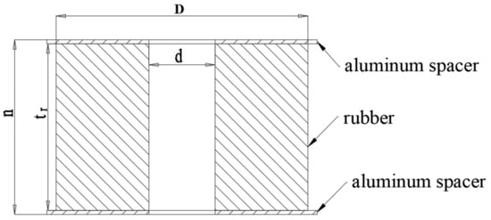
Figure 1.
Geometry of test piece construction, where D is outer diameter, d is inner diameter, tr is rubber thickness, and n is the number of rubber layers.
2.2. Experiments
This rubber buffer static test loading device utilizes a maximum test force of 100 kN and is compatible with the MTS Landmark fatigue testing machine model, as shown in Figure 2a,b. Experimental environment testing equipment using temperature and humidity meter model HTC-1.Experimental measuring equipment includes digital calipers with an accuracy of 0.01 mm. The vertical stiffness of the rubber buffers was tested in accordance with the experimental specification “General Requirements for Static Strength Tests of Aircraft Structures HB 7713-2002” [14]. Vertical compress pressure is applied gradually in three stages, with an unloading interval of 30 min between each application. This process ensures that the rubber buffer fully rebounds before the next loading. All three loading rates were set at 8 mm/min. The limiting load was the maximum load for normal use of the buffer, while the preload was 45% of the limiting load, and the limiting load was defined as 150% of the limiting load.
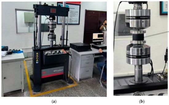
Figure 2.
The experimental setup and loading detail. (a) The experimental setup. (b) The loading detail diagram.
The first loading load was 12,388 N, which was gradually reduced to zero over a period of 30 s. The second loading force was 27,527 N, maintained for 30 s before unloading to zero. The third loading force was 41,291 N, sustained for 3 s without damage.
2.3. Simulation of Experiment
This paper uses ABAQUS2022 to establish an FE model. As shown in Figure 3, the specimen for static compression consists of a rubber layer and an aluminum spacer. The aluminum spacer is on two sides of the rubber layers. The contact mode between the rubber block and the aluminum spacer is defined by two key interactions: tangential behavior, which pertains to friction, and normal behavior, which refers to hard contact. Due to the static test, clamps are used to secure the rubber layer and aluminum spacer, preventing fluctuations in the horizontal direction. In practice, a metal rod passes through the buffer bore to connect the rubber layer in series with the aluminum spacer. Therefore, five degrees of freedom, excluding the vertical movement of the center hole of the entire specimen, are restricted by the constraints. Additionally, the lower surface of the lowest aluminum spacer is constrained in all six degrees of freedom. The meshes are composed entirely of C3D8R elements, which effectively represent the nonlinear processes involved in rubber deformation. Due to the significant deformation of the hyperelastic mesh of the rubber material, which results in pronounced geometric nonlinearities within the model, an implicit dynamics solver is employed. The vertical stiffness can be calculated during post-processing by measuring the vertical reaction force at the center of the lower surface and the vertical displacement at the center of the upper surface. Stiffness is defined as
where is the load at the end of the simulation, is the load at the end of the last simulation, is the displacement at the end of the simulation, and is the displacement at the end of the last simulation.
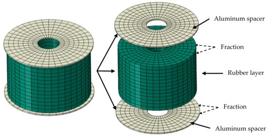
Figure 3.
Finite element model of rubber buffer.
A bilinear material with isotropic hardening was utilized to model the aluminum spacer. The Young’s modulus was set to 70 GPa, and the Poisson’s ratio was set to 0.32. In addition, the yield and ultimate strengths were 193 MPa and 228 MPa, respectively.
In this paper, the Mooney–Rivlin model is used to simulate the rubber layer material. The Mooney–Rivlin [15,16,17,18] model is one of the most commonly used intrinsic models for hyperelastic materials and is widely applied to the deformation of elastomers in engineering [19]. The mechanical properties of rubber materials can be effectively characterized within a specific range using the Mooney–Rivlin model equation.
where and are the first and second invariants of the deformation tensor, respectively. and are the material constants of rubber, and is the incompressible parameters.
The modulus of elasticity and the shear modulus of rubber materials exhibit the following relationship under specific conditions.
where is shear modulus of rubber, and is the rubber Poisson’s ratio of 0.5.
Thus, , and the relationship between and , is
Based on previous experimental data, the following relationship can be established.
The known rubber hardness can be converted to the modulus of elasticity using Formula (6). Subsequently, this can be calculated by Formula (5), provided that the ratio of the relevant parameters , is determined [20]. In practical applications, measuring rubber hardness is relatively straightforward, making it easier to obtain the material parameters using this method. Three sets of data are selected and input into ABAQUS, where Equation (5) is employed to calculate three different sets of values, as shown in the accompanying Table 1. According to the simulation results depicted in the Figure 4, it is evident that the material parameters for CS-2 are closest to the experimental values; therefore, this parameter is selected.

Table 1.
The parameters of rubber material.
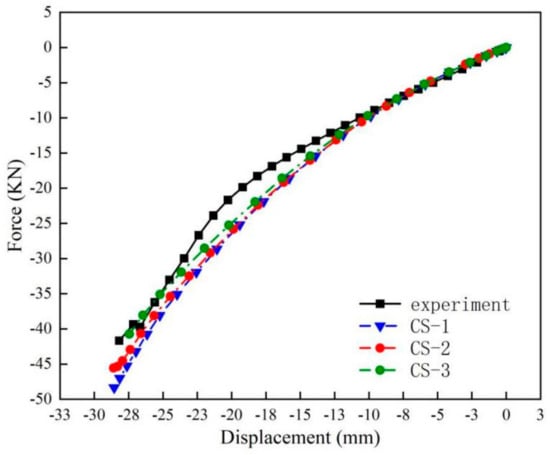
Figure 4.
Simulation of rubber buffer specimen.
The ABAQUS FE simulation of the preloading experiment, limiting load experiment, and ultimate load experiment was conducted, resulting in the load–displacement curve presented in Figure 5. The stress distribution and deformation of the rubber buffer under various vertical pressures are illustrated in Figure 6.
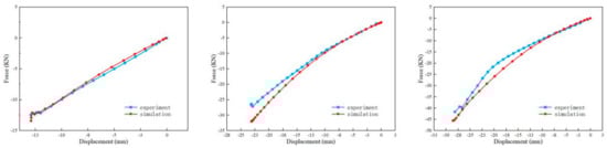
Figure 5.
Comparison between numerical and experimental results.
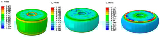
Figure 6.
Stress distribution and deformation of rubber buffers under different vertical pressures.
3. Parametric FE Analysis
3.1. Analysis Parameters
The BP neural network modeling is achieved through the iterative training of samples, necessitating the use of multiple sets of raw data. This section presents an extensive parametric analysis of the effects of vertical stiffness using the FE models discussed in the previous section. A series of three-dimensional FE models of rubber buffers were developed using ABAQUS, based on buffer specimens from previous studies. The detailed geometric parameters of the buffers are shown in Table 2. These buffers are commonly used in practical engineering. The analysis considers different values of outer diameter , rubber thickness , vertical pressure , and the number of rubber layers (n). The thickness of the aluminum spacer was kept constant for all buffers. It is important to note that while the inner diameter of the rubber buffer significantly affects stiffness, variations in the inner diameter was not considered in this study. A more comprehensive study should include the rubber buffer’s inner diameter as a critical variable. The vertical pressures applied during the experiment were 2 MPa, 4.4 MPa, and 6.6 MPa.
Table 2.
Details of FE models.
3.2. Discussion of Results
The collected force–displacement relationships of rubber buffers under different shapes are shown in Figure 7. The load from 0 to a predetermined pressure is gradually applied incrementally in the FE model. The slope of each load–displacement curve at a specific point represents the stiffness of the rubber buffer at the corresponding pressure. The collected force–displacement shows the nonlinear phenomenon of rubber.
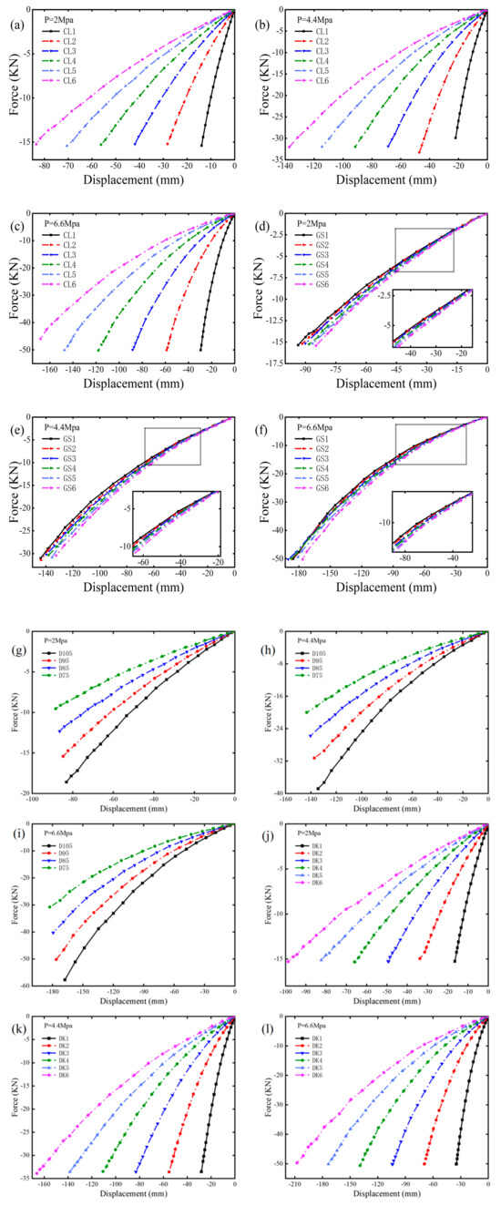
Figure 7.
FE model load–displacement curve: (a) P1 = 2 Mpa, (b) P2 = 4.4 Mpa, (c) P3 = 6.6 Mpa, (d) P1 = 2 Mpa, (e) P2 = 4.4 Mpa, (f) P3 = 6.6 Mpa, (g) P1 = 2 Mpa, (h) P2 = 4.4 Mpa, (i) P3 = 6.6 Mpa, (j) P1 = 2 Mpa, (k) P2 = 4.4 Mpa, (l) P3 = 6.6 Mpa.
The load–displacement curves derived from the rubber buffers designated as CL1 to CL6, as presented in Table 2, are shown in Figure 7a–c. The figure illustrates that the stiffness of the rubber buffers decreases with an increase in the number of rubber layers under varying loads. Furthermore, the number of rubber layers significantly influences the stiffness of the buffers.
To maintain a constant total height of the rubber buffer while increasing the number of rubber layers, the load–displacement curves for the rubber buffers designated GS1 to GS6, as presented in Table 2, are shown in Figure 7e–g. Due to the increase in the number of rubber layers, the number of layers of the aluminum spacer also increases. The increase in the number of aluminum spacers leads to an enhancement in the vertical stiffness of the buffer. Furthermore, an increase in the number of layers results in a reduction in both the vertical and lateral deformations.
In comparison to other parameters, the quantity of rubber layers exerts the least influence on the stiffness when the total height of the rubber buffer remains constant. The load–displacement curves obtained from the rubber buffers designated D105 to D75, as presented in Table 2, are shown in Figure 7g–i. It is evident that the vertical stiffness exhibits an increase corresponding to the enlargement of the outer diameter of the buffer.
The data presented in Table 2 indicate that all buffer stiffness values increase with rising vertical pressure. This observation suggests that, in addition to the shape factor of the buffer itself, the load applied to the front landing gear is a significant variable to consider when predicting buffer stiffness.
Pearson’s correlation coefficient is a statistical metric that quantifies the extent of linear correlation between two variables. The coefficient ranges from −1 to 1, where a value of 1 indicates a perfect positive correlation, −1 signifies a perfect negative correlation, and 0 denotes the absence of any linear correlation [21]. Table 3 indicates that outer diameter and vertical pressure are positively correlated with vertical stiffness. Rubber thickness and the number of rubber layers are negatively correlated with vertical stiffness. The Pearson correlation coefficients between outer diameter, rubber thickness, the number of rubber layers, vertical pressure, and the vertical stiffness are 0.170, −0.178, −0.544 and 0.357, respectively. It can be seen that the number of rubber layers and vertical pressure have a great influence on the vertical stiffness of the buffer.
Table 3.
The correlation analysis between outer diameter, rubber thickness, the number of rubber layers, vertical pressure, and the vertical stiffness.
4. Neural Network Predictions
Neural networks, as a significant component of machine learning, have diverse applications within the engineering domain [22]. Prominent types of neural networks include feedforward neural networks (RNNs), generative adversarial networks (GANs), and backpropagation neural networks (BP) [23]. The following sections provide a description of commonly utilized neural network algorithms.
CNN algorithms belong to a class of feedforward neural networks that include convolutional computation and have a deep structure [24,25,26,27]. As a prominent algorithm within the realm of deep learning, CNNs can be understood as multilayer perceptrons that optimize the number of parameters through local connectivity and weight sharing, thereby decreasing model complexity. Primarily employed in image processing tasks, CNNs necessitate substantial datasets for effective training, which is most efficiently conducted using graphics processing units (GPUs).
The RNN is a kind of recursive neural network that uses sequential data as input, recursively in the evolutionary direction of a series, in which all the nodes are connected in a chained fashion. Convolutional neural networks (CNNs) constitute a specific class of feedforward neural networks distinguished by their use of convolutional operations and a deep architectural structure [28,29,30,31,32]. As a significant algorithm in the field of deep learning, CNNs can be conceptualized as multilayer perceptrons that enhance parameter optimization through local connectivity and weight sharing, thus reducing model complexity. Predominantly utilized in image processing applications, CNNs require extensive datasets for effective training, which is most efficiently performed using graphics processing units (GPUs).
The GAN is a new framework for estimating generative models through an adversarial process. Two models are trained simultaneously in the framework. It is mainly used in image generation, data enhancement, image processing, and other fields. Despite the proliferation of new neural network techniques, choosing a suitable neural network model is the key to solving the problem. A suitable neural network algorithm can save a lot of time and computational resources while ensuring prediction accuracy. The ANN (BP) has strong nonlinear mapping (suitable for nonlinear problems) and requires less hardware than CNN algorithms [33,34,35,36].
The BP neural network was selected for this study due to its computational efficiency and suitability for addressing problems involving nonlinear relationships between input and output variables. Although convolutional neural networks (CNNs) and recurrent neural networks (RNNs) offer advantages in specific domains (e.g., image processing and sequential data), they often require more computational resources and longer training times. In contrast, the BP neural network strikes an effective balance between accuracy and computational efficiency for the specific problem, as demonstrated by its high prediction accuracy and relatively short training time. Additionally, the BP neural network’s ability to capture complex, multivariate interactions without requiring extensive computational resources makes it an optimal choice for predicting the stiffness of rubber buffers.
4.1. BP Neural Network Prediction Principle
BP neural networks are the most commonly used multilayer perceptron networks that employ error backpropagation among the various types of artificial neural networks [37]. The structure consists of one input layer, several hidden layers, and one output layer. The layers are connected by weights, and there are no connections between layers of the same type [38]. The core steps of the BP neural network model are shown in Figure 8. For the input training samples, the hidden layer is obtained by forward propagation and propagated to the output layer after the activation function is computed. If the result produced by the output layer is unsatisfactory, then it is necessary to backpropagate, adjust the weights, and retrace the original path. The error is minimized through continuous iteration, resulting in satisfactory outcomes.
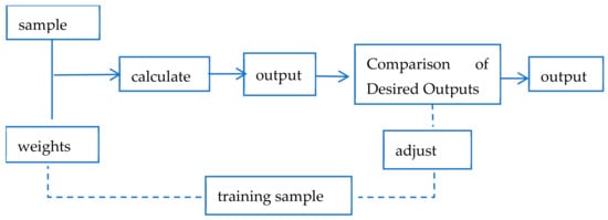
Figure 8.
BP neural network core steps.
The activation function, i.e., the Sigmoid function, is
The loss function is defined as follows:
where is the input sample, is output value, is the desired output value, is the connection weight of the neuron, and is the bias vector.
4.2. BP Neural Network Modeling
The reasonableness of the number of hidden layers in a neural network is related to the accuracy of its predictions. The empirical formula was used to determine the range of the number of neurons in the single hidden layer, which was 5–13. Then, the trial and error method was used to determine the optimal number of neurons in the single hidden layer, which was five and four, respectively [39]. The incorporation of additional hidden layers in deeper neural networks heightens the risk of overfitting. In scenarios where the dataset is limited in size, shallower networks, such as those with a single hidden layer, may be insufficient to adequately capture the intricate nonlinear relationships that exist between input parameters and their corresponding outputs. The BP neural network model structure consists of an input layer, two hidden layers, and an output layer. The input layer is composed of diameter , rubber thickness , vertical pressure , and the number of rubber layers , and the output layer is composed of vertical stiffness . A schematic representation of the neural network model is presented in Figure 9.
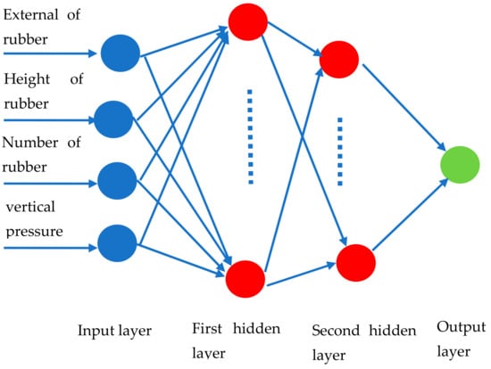
Figure 9.
Schematic diagram of BP neural network structure.
To mitigate prediction errors in large neural networks that arise from substantial fluctuations in input data and to enhance both the accuracy and the speed of predictions, it is necessary to normalize the input data [40]. The normalization process is conducted using the formula shown in Formula (9).
where is the maximum of the desired outcome, is the minimum of the desired outcome, is the maximum value of the original data, is the minimum value of the original data, and is the normalized data.
4.3. BP Neural Network Model Training
In the BP neural network, the number of initial data significantly impacts the network’s performance. Thus, 42 sets of data were derived from the FE model, BP neural network modeling is achieved through the iterative training of raw data. To mitigate the risk of overfitting, the dataset was partitioned into a training set comprising 75% of the data and a test set comprising 25%. The training set is utilized for model training, whereas the test set serves to assess the model’s performance on previously unseen data. This approach is instrumental in ensuring that the model generalizes effectively to new data. Throughout the training process, the error associated with the validation set is closely monitored. If an increase in validation error is observed while the training error continues to decline, the training process is halted to avert overfitting. This methodology ensures that the model does not inadvertently learn the noise present in the training data. The number of training iterations is set to 1000, the learning rate to 0.03, and the minimum acceptable error for the training objective to .
The model stops fitting when the number of iterations is about 10, and the best results are obtained at the fourth iteration of training. The BP neural network model, trained using the sample data, demonstrates the capability to compute the vertical stiffness of the rubber buffer. To validate the trained BP neural network model, it is essential to evaluate the model using a test set; specifically, the remaining 11 data points are used to test the BP neural network model. The test results are shown in the Figure 10.
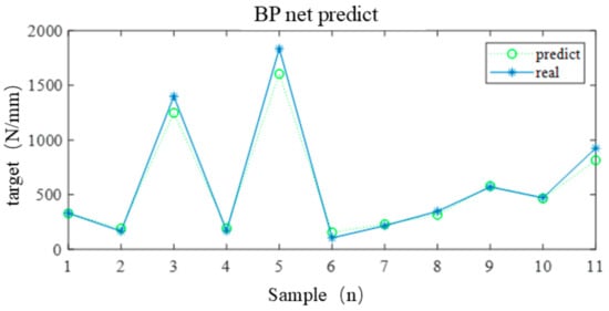
Figure 10.
Comparison of actual and predicted vertical stiffness values.
This shows that the predicted values closely align with the 11 values used for testing, and the associated error remains within an acceptable range. It is evident that the training effect for buffer stiffnesses up to 500 N/mm is less pronounced than that for stiffnesses exceeding 500 N/mm. This discrepancy can be attributed to the limited training dataset, which includes a smaller number of buffers with stiffnesses greater than 500 N/mm.
It can be seen from Figure 11 that the target value is the training accuracy, and the best value is the highest accuracy that can be achieved during the training process across the training set, validation set, and test set. The horizontal coordinate value in the training process represents the number of iterations, and the vertical coordinate represents the mean squared error. It can be seen that the best value after training exceeds the target value and meets the requirements. From Figure 12, it can be seen that the training set, validation set, test set, and total dataset are fitted after training. The correlation coefficient R between the prediction results and the finite element results is close to 1, which indicates that the error between the output values and the finite element results is very small.
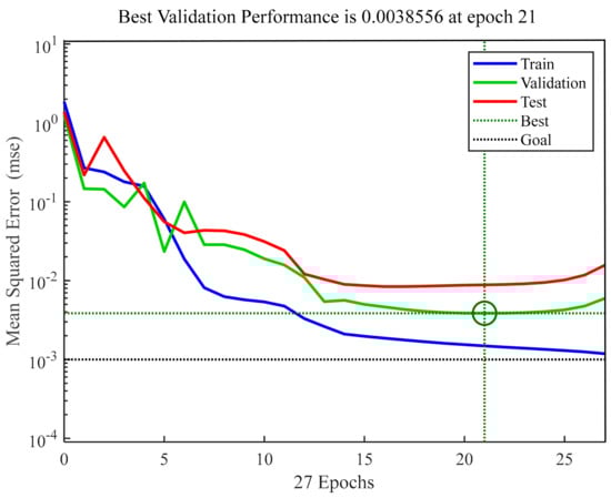
Figure 11.
Image of error variation during network training.
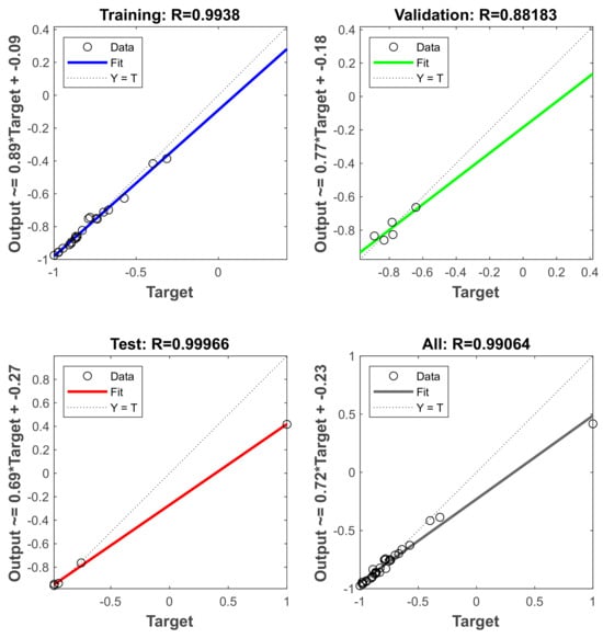
Figure 12.
Correlation analysis results.
In machine learning, the prediction results are usually judged by comparing the predicted values with the output values. The following indicators are generally selected for evaluation: coefficient of determination (); is the ratio of the sum of the squares of the regression to the sum of the squares of the total deviations in a linear regression, namely
while is a criterion for the goodness of fit of the regression equation. So, the closer is to 1, the better the algorithm’s prediction result.
According to Figure 13, the coefficient of determination resulting from the training of the BP neural network is . It shows that the error between the predicted and actual values is minimal. In addition, the slope of the fitted equation is closer to 1, indicating that the error between the predicted and actual values is more petite. It is evident that the neural network can be effectively trained to establish the relationship between the outer diameter , rubber thickness , vertical pressure , the number of rubber layers , and the vertical stiffness of the rubber buffer.
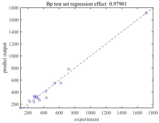
Figure 13.
BP test set regression effect.
5. Comparison Between BP Network and Formula
According to “rubber bearing part 3: Building Seismic Isolation Rubber Bearing GB 20688.3-2006” [41], the formula for calculating the vertical stiffness of the rubber bearings is as follows:
where is the bonded rubber area, is the number of rubber bearings, is the thickness of one rubber layer, and is the modified compression modulus of the elasticity of the rubber, defined as follows:
where is the elastic modulus in compression; is the bulk modulus of the elasticity valued references [42].
where is the shear modulus of the rubber valued references, and is a correction factor related to the hardness of the rubber; is the first shape factor, which is defined as the ratio of the constrained area to the force-free area of the single layer of rubber. , , and are defined as follows:
where is the external diameter of the rubber layer, and d is the inside diameter of the rubber layer.
A total of 12 groups of buffers were randomly selected, and the vertical stiffness of the rubber buffers was calculated using the aforementioned formula. The errors associated with the finite element model error are shown in Table 4. It can be seen in “rubber bearing part 3: Building Seismic Isolation Rubber Bearing GB 20688.3-2006” that the buffer formula given by the finite element analysis exhibited a minimum error of 67.59% and a maximum error of 88.36%. This formula exhibits a significant calculation error, rendering it unsuitable for calculating the stiffness of a rubber buffer. Additionally, it fails to account for vertical pressure as a factor influencing stiffness. From Table 5, it can be seen that the accuracy of the BP neural network model in predicting the vertical stiffness of the rubber buffer is much higher than that of the traditional formula. The error falls within an acceptable range, indicating that the BP neural network model is more effective in addressing the multivariate linear coupling relationships compared to traditional formulas. The model demonstrates a strong capacity for generalization across various buffer geometries within the confines of the training data. Future research endeavors may involve the expansion of the dataset to encompass a broader spectrum of geometries and loading conditions, thereby enhancing the model’s generalization capabilities. To further validate the selection of the neural network, the performance of the BP neural network was compared to that of a polynomial regression model utilizing the same dataset. The results indicate that the polynomial regression model encounters difficulties in capturing nonlinear relationships, resulting in higher prediction errors in comparison to the neural network. This finding suggests that, particularly when addressing complex multivariate interactions, simpler methodologies may be inadequate for accurately predicting the stiffness of rubber buffers.
Table 4.
Traditional formulations and FE model results and relative errors.
Table 5.
BP neural network and finite element results and relative errors.
6. Conclusions
The vertical stiffness relationship of airplane rubber buffers under the combined effect of outer diameter, rubber thickness, vertical pressure, and the number of rubber layers is established for the first time based on the compression simulation of an FE model. BP neural networks are used for the first time to explore the vertical stiffness relationships of rubber materials. The results of the predictions were compared with those obtained using traditional formulas. The primary conclusions are as follows:
The rubber exhibits an increasing vertical stiffness phenomenon, and the vertical stiffness increases with the vertical pressure due to the hyperelasticity property. This observation suggests that, in addition to the shape factor of the buffer itself, the load applied to the front landing gear is a significant variable to consider when predicting buffer stiffness.
Outer diameter and vertical pressure are positively correlated with vertical stiffness. Rubber thickness and the number of rubber layers are negatively correlated with vertical stiffness. The number of rubber layers and the application of vertical pressure significantly affect the vertical stiffness of the buffer. In contrast, the thickness of the rubber and the outer diameter exert a lesser influence on the vertical stiffness of the buffer.
The optimal hidden layer number of the BP neural network is two, with the corresponding numbers of neurons being five and four, respectively. The predicted values exhibit a strong correlation with the FE model, and the associated errors remain within acceptable thresholds. A comparative analysis demonstrates that the prediction accuracy of the BP neural network is between 67.59% and 88.5% higher than that of the traditional formulas. Although simpler response surface methods may be employed to model the stiffness of rubber buffers, they do not achieve the same degree of accuracy as neural networks; this is mainly due to the nonlinear and multivariate characteristics of the problem. The determination of numerous parameters in neural networks frequently depends on prior knowledge and experience, which may affect the objectivity and accuracy of the assessment. This issue is not comprehensively addressed in this paper. Advanced neural network theory may provide more insight into this matter.
Author Contributions
Conceptualization, Z.H.; methodology, software, Z.H., and S.Z. and H.M.; validation, Z.H.; data curation, Z.H.; writing—original draft preparation, X.X.; writing—review and editing, Z.H.; supervision, X.X.; project administration, X.X. All authors have read and agreed to the published version of the manuscript.
Funding
This research was funded by Liaoning General Aviation Research Institute Shenyang Aerospace University. And the APC was funded by Liaoning General Aviation Research Institute Shenyang Aerospace University.
Data Availability Statement
The raw data supporting the conclusions of this article will be made available by the authors on request.
Conflicts of Interest
The authors declare no conflict of interest.
References
- Gudmundsson, S. General Aviation Aircraft Design: Applied Methods and Procedures; Butterworth-Heinemann: Oxford, UK, 2013; pp. 480–485. [Google Scholar]
- Can, Z.J.; Huang, Z.W.; Yu, J.H.; Gao, Z.J. The 14th Fascicule of Aircraft Design Manual: Take-Off and Landing System Design; Aviation Industry Press: Beijing, China, 2002; pp. 95–107. [Google Scholar]
- Lee, J.; Park, H.; Kim, S.-J.; Kwon, Y.-N.; Kim, D. Numerical investigation into plastic deformation and failure in aluminum alloy sheet rubber-diaphragm forming. Int. J. Mech. Sci. 2018, 142, 112–120. [Google Scholar] [CrossRef]
- Xu, X.; Yao, X.; Dong, Y.; Yang, H.; Yan, H. Mechanical behaviors of non-orthogonal fabric rubber seal. Compos. Struct. 2021, 259, 113453. [Google Scholar] [CrossRef]
- Liu, Y.; Zhang, Q.; Liu, R.; Chen, M.; Zhang, C.; Li, X.; Li, W.; Wang, H. Compressive stress-hydrothermal aging behavior and constitutive model of shield tunnel EPDM rubber material. Constr. Build. Mater. 2022, 320, 126298. [Google Scholar] [CrossRef]
- Hu, Y.; Zhu, H.; Zhu, W.; Li, C.; Pi, Y. Dynamic performance of a multi-ribbed belt based on an overlay constitutive model of carbon-black-filled rubber and experimental validation. Mech. Syst. Signal Process. 2017, 95, 252–272. [Google Scholar] [CrossRef]
- Luo, Y.; Liu, Y.; Yin, H. Numerical investigation of nonlinear properties of a rubber absorber in rail fastening systems. Int. J. Mech. Sci. 2013, 69, 107–113. [Google Scholar] [CrossRef]
- Wang, J. Mechanical Properties and Stability Analysis of Thick Laminated Rubber Seismic Isolation Bearing. Master’s Thesis, Guangzhou University, Guangzhou, China, 2020. [Google Scholar]
- Wang, Y.; Shen, C.; Huang, X. Calculation of vertical stiffness of thick rubber seismic isolation bearings and analysis of their influencing factors. South China Earthq. 2023, 43, 132–142. [Google Scholar]
- Chen, L.; Cui, L.; Chen, Y.; Wang, Y.; Ke, K. BP Neural Network Prediction of Vertical Stiffness of Rubber Seismic Isolation Bearing. J. Archit. Civ. Eng. 2023, 40, 84–90. [Google Scholar]
- Yuan, Z.; Niu, M.-Q.; Ma, H.; Gao, T.; Zang, J.; Zhang, Y.; Chen, L.-Q. Predicting mechanical behaviors of rubber materials with artificial neural networks. Int. J. Mech. Sci. 2023, 249, 108265. [Google Scholar] [CrossRef]
- Versaci, M.; Laganà, F.; Morabito, F.C.; Palumbo, A.; Angiulli, G. Adaptation of an Eddy Current Model for Characterizing Subsurface Defects in CFRP Plates Using FEM Analysis Based on Energy Functional. Mathematics 2024, 12, 2854. [Google Scholar] [CrossRef]
- Angiulli, G.; Calcagno, S.; De Carlo, D.; Laganá, F.; Versaci, M. Second-order parabolic equation to model, analyze, and forecast thermal-stress distribution in aircraft plate attack wing–fuselage. Mathematics 2019, 8, 6. [Google Scholar] [CrossRef]
- CCAR-23-R3. Civil Aviation Regulations of China Part 23: Airworthiness Standards for Normal, Utility, Aerobatic, and Commuter Aircraft. 2004. Available online: http://www.caac.gov.cn/XXGK/XXGK/MHGZ/201511/t20151102_8500.html (accessed on 10 February 2025).
- van Tonder, J.D.; Venter, M.P.; Venter, G. A novel method for resolving non-unique solutions observed in fitting parameters to the Mooney Rivlin material model. Finite Elem. Anal. Des. 2023, 225, 104006. [Google Scholar] [CrossRef]
- Manan, N.; Noor, S.; Azmi, N.N.; Mahmud, J. Numerical investigation of Ogden and Mooney-Rivlin material parameters. ARPN J. Eng. Appl. Sci. 2015, 10, 6329–6335. [Google Scholar]
- Sun, Y.; Chen, L.; Yick, K.-L.; Yu, W.; Lau, N.; Jiao, W. Optimization method for the determination of Mooney-Rivlin material coefficients of the human breasts in-vivo using static and dynamic finite element models. J. Mech. Behav. Biomed. Mater. 2019, 90, 615–625. [Google Scholar] [CrossRef]
- Bin, D.X.; Zhao, Y.Q.; Lin, F.; Xiao, Z. Parameters determination of Mooney-Rivlin model for rubber material of mechanical elastic wheel. Appl. Mech. Mater. 2017, 872, 198–203. [Google Scholar]
- Wang, W.; Deng, T.; Zhao, S. Determination of material constants in the Mooney-Rivlin model of rubber. Spec. Rubber Prod. 2004, 25, 8–10. [Google Scholar]
- Huang, Q. Rubber Mooney-Rivlin model and its coefficient least squares solution. Trop. Agric. Sci. 2009, 29, 20–24. [Google Scholar]
- Zhang, M.; Li, W.; Zhang, L.; Jin, H.; Mu, Y.; Wang, L. A Pearson correlation-based adaptive variable grouping method for large-scale multi-objective optimization. Inf. Sci. 2023, 639, 118737. [Google Scholar] [CrossRef]
- Guha, S.; Jana, R.K.; Sanyal, M.K. Artificial neural network approaches for disaster management: A literature review. Int. J. Disaster Risk Reduct. 2022, 81, 103276. [Google Scholar] [CrossRef]
- De Albuquerque Filho, J.E.; Brandão, L.C.P.; Fernandes, B.J.T.; Maciel, A.M.A. A review of neural networks for anomaly detection. IEEE Access 2022, 10, 112342–112367. [Google Scholar] [CrossRef]
- Seo, Y.M.; Pandey, S.; Lee, H.U.; Choi, C.; Park, Y.G.; Ha, M.Y. Prediction of heat transfer distribution induced by the variation in vertical location of circular cylinder on Rayleigh-Bénard convection using artificial neural network. Int. J. Mech. Sci. 2021, 209, 106701. [Google Scholar] [CrossRef]
- Jalal, M.; Moradi-Dastjerdi, R.; Bidram, M. Big data in nanocomposites: ONN approach and mesh-free method for functionally graded carbon nanotube-reinforced composites. J. Comput. Des. Eng. 2019, 6, 209–223. [Google Scholar] [CrossRef]
- Jodaei, A.; Jalal, M.; Yas, M.H. Free vibration analysis of functionally graded annular plates by state-space based differential quadrature method and comparative modeling by ANN. Compos. Part B Eng. 2012, 43, 340–353. [Google Scholar] [CrossRef]
- Weng, H.; Luo, C.; Yuan, H. ANN-aided evaluation of dual-phase microstructural fabric tensors for continuum plasticity representation. Int. J. Mech. Sci. 2022, 231, 107560. [Google Scholar] [CrossRef]
- Sherstinsky, A. Fundamentals of recurrent neural network (RNN) and long short-term memory (LSTM) network. Phys. D Nonlinear Phenom. 2020, 404, 132306. [Google Scholar] [CrossRef]
- Yin, W.; Kann, K.; Yu, M.; Schütze, H. Comparative study of CNN and RNN for natural language processing. arXiv 2017, arXiv:1702.01923. [Google Scholar]
- Kattenborn, T.; Leitloff, J.; Schiefer, F.; Hinz, S. Review on Convolutional Neural Networks (CNN) in vegetation remote sensing. ISPRS J. Photogramm. Remote Sens. 2021, 173, 24–49. [Google Scholar] [CrossRef]
- Alzubaidi, L.; Zhang, J.; Humaidi, A.J.; Al-Dujaili, A.; Duan, Y.; Al-Shamma, O.; Santamaría, J.; Fadhel, M.A.; Al-Amidie, M. Review of deep learning: Concepts, CNN architectures, challenges, applications, future directions. J. Big Data 2021, 8, 1–74. [Google Scholar] [CrossRef] [PubMed]
- Rahul, C.; Ghanshala, K.K.; Joshi, R.C. Convolutional neural network (CNN) for image detection and recognition. In Proceedings of the 2018 First International Conference on Secure Cyber Computing and Communication (ICSCCC), Jalandhar, India, 15–17 December 2018; IEEE: Piscataway, NJ, USA, 2018. [Google Scholar]
- Kurucan, M.; Özbaltan, M.; Yetgin, Z.; Alkaya, A. Applications of artificial neural network based battery management systems: A literature review. Renew. Sustain. Energy Rev. 2024, 192, 114262. [Google Scholar] [CrossRef]
- Song, H.; Ahmad, A.; Farooq, F.; Ostrowski, K.A.; Maślak, M.; Czarnecki, S.; Aslam, F. Predicting the compressive strength of concrete with fly ash admixture using machine learning algorithms. Constr. Build. Mater. 2021, 308, 125021. [Google Scholar] [CrossRef]
- Alsarraf, J.; Moayedi, H.; Rashid, A.S.A.; Muazu, M.A.; Shahsavar, A. Application of PSO–ANN modelling for predicting the exergetic performance of a building integrated photovoltaic/thermal system. Eng. Comput. 2020, 36, 633–646. [Google Scholar] [CrossRef]
- Panahi, F.; Ahmed, A.N.; Singh, V.P.; Ehtearm, M.; Elshafie, A.; Haghighi, A.T. Predicting freshwater production in seawater greenhouses using hybrid artificial neural network models. J. Clean. Prod. 2021, 329, 129721. [Google Scholar] [CrossRef]
- Li, J.; Cheng, J.-H.; Shi, J.-Y.; Huang, F. Brief introduction of back propagation (BP) neural network algorithm and its improvement. In Advances in Computer Science and Information Engineering; Springer: Berlin/Heidelberg, Germany, 2012; Volume 2. [Google Scholar]
- Goh, A.T.C. Back-propagation neural networks for modeling complex systems. Artif. Intell. Eng. 1995, 9, 143–151. [Google Scholar] [CrossRef]
- Shen, H.; Wang, Z.; Gao, C.; Qin, J.; Yao, F.; Xu, W. Determining the number of BP neural network hidden layer units. J. Tianjin Univ. Technol. 2008, 24, 13. [Google Scholar]
- Huang, L.; Qin, J.; Zhou, Y.; Zhu, F.; Liu, L.; Shao, L. Normalization techniques in training dnns: Methodology, analysis and application. IEEE Trans. Pattern Anal. Mach. Intell. 2023, 45, 10173–10196. [Google Scholar] [CrossRef]
- GB 20688.3; Rubber Bearings Part 3: Seismic Isolation Rubber Bearings for Buildings. General Administration of Quality Supervision, Inspection and Quarantine: Beijing, China, 2006.
- Lindley, P.B. Natural rubber structural bearings. Spec. Publ. 1981, 70, 353–378. [Google Scholar]
Disclaimer/Publisher’s Note: The statements, opinions and data contained in all publications are solely those of the individual author(s) and contributor(s) and not of MDPI and/or the editor(s). MDPI and/or the editor(s) disclaim responsibility for any injury to people or property resulting from any ideas, methods, instructions or products referred to in the content. |
© 2025 by the authors. Licensee MDPI, Basel, Switzerland. This article is an open access article distributed under the terms and conditions of the Creative Commons Attribution (CC BY) license (https://creativecommons.org/licenses/by/4.0/).