Abstract
This paper presents an innovative aeroelastic solution method called the implicit dynamic approach (IDA). The IDA is a novel technique implemented to address the complexities of structural displacement and fluid–structure interactions. At the core of this method lie the Navier–Stokes equations, which are pivotal for resolving the unsteady aerodynamic forces for studying aeroelasticity. This paper develops a time-step-coupling data-solving interface that bridges the structural dynamic and fluid dynamic domains, ensuring a seamless integration of these two critical aspects of aeroelastic analysis. To substantiate the credibility of the IDA, the aeroelastic responses of a two-dimensional wing and the benchmark supercritical wing (BSCW) are analyzed. The results obtained from these models demonstrate the IDA’s credibility and stability. The IDA proves to be reliable in predicting aeroelastic responses and offers a powerful tool for analyzing aeroelastic problems.
1. Introduction
Aeroelasticity concerns physical phenomena involving significant mutual interactions among inertial, elastic, and aerodynamic forces. There are many solution methods of aeroelasticity, which can generally be classified as either frequency domain or time domain methods. The frequency domain methods include the p-k method [1], the modified p-k method [2], the V-g method, and the g method [3]. In frequency domain methods, the unsteady aerodynamic forces are usually calculated using the doublet lattice method [4], which is based on linear aerodynamic theories [5]. The frequency domain methods are suitable for solving systems in the critical state but cannot accurately solve systems under the subcritical or supercritical condition [6]. The calculation number of frequency domain methods is low, which is suitable for engineering design. However, time domain methods have become increasingly important in recent years, and the most representative of them is a coupling method for computational fluid dynamics (CFD) and computational structural dynamics (CSD). CFD uses the finite volume method to solve the Navier–Stokes equations in their integral form, and CSD usually applies finite element analysis to calculate the structural vibration response. Some interpolation methods are used for data exchange at the interface. In the past 20 to 30 years, a significant amount of research has been conducted on CFD/CSD-coupling approaches. Many scholars have used CFD/CSD-coupling approaches to solve aeroelastic problems. For example, Bosch et al. [7] used a numerical modeling approach (CFD/CSD) to analyze the dynamic nonlinear aeroelastic behavior of tethered inflatable wings. Brüderlin et al. [8] presented methods and tools for direct aeroelastic simulations (CFD/CSD) to study the robust active controller stability region of a winglet. Smith [9] provided a systematic analysis of the numerical errors introduced by the data interface for high-aspect-ratio blades undergoing multibody dynamic motion, including rotation. She demonstrated that failure to consider the conservation of work or energy during CFD/CSD data exchange could lead to a shift in the mean loading, as observed for fixed-wing applications, and an alteration of the controls necessary to achieve rotor trim, affecting the rotor performance prediction. Zhang et al. [10] applied a fully coupled method using Navier–Stokes simulations to investigate the aeroelastic stability of the J-2S rocket nozzle. Wang et al. [11] developed a coupled aeroelastic modeling framework by implementing the necessary structural dynamic component in an anchored CFD methodology for transient nozzle flow analysis. De Castro et al. [12] presented a strongly coupled partitioned method for fluid–structure interactions. Zhang et al. [13] proposed two better weak coupling algorithms based on the polynomial extrapolation of generalized aerodynamic forces. Liu et al. [14] developed a time-efficient coupling scheme based on radial basis function interpolations. Xie et al. [15] developed a reduced-order model based on Volterra series for nonlinear unsteady aerodynamic analysis. Yang and Zhang [16] proposed a high-efficiency and -accuracy method based on CFD/CSD to solve the forced response. Huang et al. [17] used CFD/CSD-coupling approaches to investigate the energy-harvesting performance of a piezoelectric free-flying aircraft model. Naseri et al. [18] presented a semi-implicit coupling technique which strongly couples the added-mass term of the pressure to the elastic structure. Vindignia et al. [19] developed a novel finite element approach for the computational aeroelastic analysis of flexible lifting structures in subsonic flows. Mozaffari-Jovin et al. [20] studied the aeroelastic interaction of a locally distributed, flap-type control surface with aircraft wings operating in a subsonic potential flow field. All these studies mainly focus on the modal-based structural dynamic solution, which is highly dependent on the structural mode. Meanwhile, most of the existing CFD/CSD-coupling approaches are based on the linear multistep method [13], precise integration method [21], and Runge–Kutta method [22], which are conditionally stable and are unsuitable for the stiffness problem that requires a very small time step to solve. The accuracy of the calculation results mainly depends on the selection of the structural mode and time step, while the method proposed in this paper does not depend on the structural mode or time step.
The implicit dynamic method is usually used to solve problems involving structural forced vibration under external loads. This method has been widely recognized for its versatility in addressing a spectrum of complex engineering problems. Recent scholarly work has highlighted its diverse applications across various fields. Sha et al. [23] conducted a study employing the implicit dynamic method to tackle frictional contact impact problems characterized by large elastoplastic deformations. Lavrenčič and Brank [24,25] used implicit structural dynamic time-stepping schemes to study the shell-buckling process and applied the implicit dynamic method to analyze the post-bulking of shells. Tian et al. [26] adopted an implicit robust difference method to study the modified Burges model with nonlocal dynamic properties. Marino et al. [27] applied an implicit dynamic method to propose a novel approach to study shear-deformable geometrically exact beams. Collectively, these studies underscore the robustness and adaptability of the implicit dynamic method in solving a broad range of dynamic problems in engineering and physics. The ability of the implicit dynamic method to handle complex geometries, material nonlinearities, and large deformations makes it an invaluable tool in advanced computational mechanics.
In this paper, we propose an IDA for aeroelastic analysis, based on the simplicity dynamic method. The IDA is essentially a method that couples CFD and CSD. The CFD part uses the finite volume method to solve the Navier–Stokes equations. The CSD part uses an implicit dynamic method to solve the structural motion of the equation. Compared with low-order modeling [19,20], the method in this paper has three advantages. First, this method develops a time-step-coupling data-solving interface that effectively bridges the structural dynamic and fluid dynamic domains. Second, this method is a general approach that can be applied to a wide range of aeroelastic problems, including complex geometries and unsteady flow conditions. Third, this method is based on the Navier–Stokes equations, which are essential for resolving unsteady aerodynamic forces. The most significant advantage of the IDA is that it does not depend on the structural modal selection or time steps, which can offer certain advantages over the existing dynamic method. It is based on the formulation of the governing equation in an implicit manner, which can lead to more stable and accurate solutions, especially in cases where the system is subjected to large deformations or in complex load cases.
2. Methodology
The first part of this section briefly describes how the Navier–Stokes equations are derived using the three basic conservation laws of fluid mechanics [28]. The second part explains in detail how the structural dynamic equation is derived from the d’Alembert principle and how the IDA can be used to solve it.
2.1. Unsteady Aerodynamic Equation
In CFD, the mass equation, also known as the continuity equation, is a fundamental equation that describes the conservation of mass in a Newtonian fluid:
where is the air density, and is the flow velocity vector, with , where u, v, and w are the flow velocities in Cartesian coordinate system directions, and is the normal direction of the boundary surface.
The momentum equation is a fundamental equation that describes the motion of a Newtonian fluid. It is based on Newton’s second law of motion, which states that the force acting on a fluid element equals the rate of the change in its momentum as follows:
where p is the atmospheric pressure, , is the specific heat ratio, is the total energy, and is the viscous stress.
The energy equation is also crucial for describing the transfer and conservation of energy in a Newtonian fluid. The energy equation accounts for various forms of energy, including kinetic energy, internal energy, and potential energy. It considers the effects of the heat transfer, work done by the fluid, and energy dissipation due to viscous forces as follows:
where is the coefficient of the thermal conductivity, and T is the temperature.
Combining Equations (1)–(3), the Navier–Stokes equations can be obtained in integral form as follows:
Equation (4) can be solved using the finite volume method. The finite volume method is founded on the principle of conserving physical quantities within a control volume. This principle dictates that the computational domain is divided into non-overlapping control volumes. By integrating the Navier–Stokes equations over each control volume, we derive algebraic equations that relate the values of the flow variables at the control volume’s surface. For transient simulations, it is necessary to discretize the governing equations in both space and time. Spatial discretization is achieved using a second-order upwind scheme, which is suitable for capturing the convective terms accurately. Temporal discretization involves integrating each term in the differential equations over a time step. It employs an implicit time integration scheme, ensuring stability and accuracy in the simulation of unsteady flows. To account for the complex effects of turbulence on aerodynamic forces, the Spalart–Allmaras turbulence model is utilized. The Spalart–Allmaras model [29] is a one-equation model that solves a modeled transport equation for the kinematic turbulent viscosity. The Spalart–Allmaras model was designed specifically for aerospace applications involving wall-bounded flow and has been shown to give good results for boundary layers subjected to adverse pressure gradients.
where is the transport variable in the Spalart–Allmaras model. The model constants are , , , , , , and . The turbulent viscosity () is computed from
where is the molecular kinematic viscosity.
In both time-marching aeroelastic calculations, the mesh must be updated at each time step to reflect the dynamic changes in the flow field. This mesh deformation is accomplished using the spring method, which provides an efficient way to maintain the integrity of the computational grid while accommodating fluid–structure interactions.
2.2. IDA Method
Implicit direct-integration dynamic analysis can be used to study the structural dynamic response and flutter. Flutter is the dynamic of an elastic structure in an airflow, with the primary focus on the endemic instability of the structure [30], and it is essentially a structural vibration problem. Therefore, theoretically, the IDA could be used to solve flutter problems. Flutter is a behavior that results from the coupling of the inertial force (), elastic force (), and unsteady aerodynamic force (). In addition, the structural damping force () should be considered. The d’Alembert principle [31] is used to form the dynamic equilibrium equation as follows:
Assuming is a virtual velocity field and applying the virtual work principle [32], the following equation can be obtained:
where is the current density of the material at a given point; , , and are, respectively, the displacement, velocity, and acceleration at the point; is the current damping of the structure at the point; and is the frequency at the point.
Finite element approximation is based on interpolations, whereby the displacement, position, and other variables at any material point are defined by a finite number of nodal variables. This paper uses uppercase superscripts to refer to individual nodal variables or nodal vectors. Hence, the displacement field can be written as , where , with n ranging from 1 to the total number of variables, is a set of vector interpolation functions (shape functions), and is a set of nodal displacements. The following equations can be obtained using the variation principle:
where n is the index of the shape function, and m is the index of the nodal displacement.
Implicit operators available for the time integration of the dynamic problem include the Hilbert–Hughes–Taylor operator [33] and the backward Euler operator. The Hilbert–Hughes–Taylor operator is a generalization of the Newmark operator with controllable numerical damping (the damping being the most valuable in the automatic time-stepping scheme) because the slight high-frequency numerical noise inevitably introduced when the time step is changed is removed rapidly by a small amount of numerical damping.
where is the sum of all the Lagrange multiplier forces associated with the degree of freedom (n). The operator definition is completed using the Newmark formula for displacement and velocity integration as follows:
where , , and .
2.3. CFD/IDA-Coupling Approach
CFD/CSD-coupling strategies are broadly classified under two categories: the monolithic approach and the partitioned approach. The latter integrates available disciplinary algorithms and reduces code development time by taking advantage of the “legacy” codes or numerical algorithms that have been validated and used for solving many complicated fluid or structural problems [34]. In this paper, the CFD/IDA-coupling strategies adopt the partitioned approach, for which Figure 1 provides the procedure.
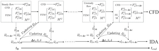
Figure 1.
The procedure of CFD/IDA coupling.
The detailed explanation of the procedure of CFD/IDA coupling is given below:
- (1)
- Initializing the flow field and calculating the steady aerodynamic forces. First, the initialization of the flow field is performed and the calculation of the aerodynamic forces are carried out under the given flow dynamic pressure condition. The characteristics of the steady flow field are computed to obtain the pressure distribution on the outer surface of the aircraft. Thus, the steady aerodynamic forces at the initial moment are calculated. At the same time, the finite element method can be used to calculate the mechanical properties, mass properties of the structure, and external force of the structure at the initial time;
- (2)
- Calculating the initial acceleration. According to Newton’s second theorem, the acceleration value at the initial moment is calculated. The acceleration response at the next moment is set to be the same as that at the initial moment;
- (3)
- Applying the procedure of the IDA. Given the time step and Newmark- parameters, the implicit numerical integration method is used to calculate the displacement value, velocity value, and acceleration value at the next moment;
- (4)
- Updating the acceleration value and external forces. The calculated acceleration value is next used to update the initial calculation value. The acceleration and the updated acceleration values are used for the external forces at the next moment, so the calculation is advanced;
- (5)
- Iterating the coupling procedure. The above steps are repeated until the calculation time reaches the required total time. At the total time, the calculation is stopped, and the aeroelastic response results are outputted for the entire time period.
Unlike the previous CFD/CSD-coupling idea, the solution idea in this paper is based on the implicit dynamic method, which has good stability. This makes the solution result highly reliable, portable, and able to be parallelized.
3. Results and Discussion
3.1. The Two-Dimensional Wing
In previous studies, two-dimensional wings [35,36,37] have usually been used in basic theoretical research on aeroelasticity. In this paper, a two-dimensional wing (Figure 2) is used to validate the reliability of the IDA. Table 1 lists the structural parameters of the two-dimensional wing. The mid-chord length is 1.00 m, the elastic center’s location coefficient is −0.10, the center of gravity’s location coefficient is 0.25, and the non-dimensional radius of gyration is . The plunge and pitch vibration circular frequencies are 25.00 rad/s and 50.00 rad/s, respectively, and and are defined as uncoupled still-air frequencies. Figure 3 shows the two modes of the two-dimensional wing.

Figure 2.
The two-degree-of-freedom mechanical model of the wing.

Table 1.
The structural parameters of the two-dimensional wing.

Figure 3.
The structural modes of the two-dimensional wing. (a) Plunge mode; (b) pitch mode.
To compute the unsteady aerodynamic forces, the fluid mesh (Figure 4) of the two-dimensional wing was established with 7584 cells and 7680 nodes. The solver codes were written for this work, and a data exchange interface was pre-reserved just for the IDA analysis. It should be noted that the flutter velocity is lower than a Mach number of 0.2, as inferred from the result of the frequency domain analysis. This is why incompressible fluids’ Navier–Stokes equations were selected, which are also straightforward to implement in code. Figure 5 shows the fluid velocity of a steady flow and the dynamic pressure of a steady flow before the flutter analysis. Figure 6 shows the lift coefficient, pitch moment coefficient, and aerodynamic centers of different angles of attack (AOAs). All these data show that the aerodynamic mesh is effective and can be used for subsequent unsteady aerodynamic calculations.

Figure 4.
The fluid mesh of the two-dimensional wing (7584 cells and 7680 nodes).

Figure 5.
The fluid condition of the two-dimensional wing. (a) Flow velocity; (b) dynamic pressure.

Figure 6.
The flow characteristics at different AOAs. (a) Lift coefficient; (b) pitch moment coefficient; (c) aerodynamic center’s location.
Flutter analyses were conducted at different dynamic pressures, assuming the ideal gas condition. The time–displacement response was obtained using the IDA. Using these data, Fourier analysis was applied to generate frequency response curves. Figure 7 plots the time–displacement and frequency response curves. According to the results, when the dynamic pressure is 1600 Pa, the time–displacement response is close to equal to the amplitude oscillation. When the dynamic pressure is over 1600 Pa, it gradually becomes higher. Hence, the time–displacement response is close to the constant amplitude oscillation. The 1600 Pa pressure is the critical flutter dynamic pressure, which is converted to a flow velocity of 51.0 m/s. Figure 8 gives the damping and circular frequency curves at different dynamic pressures. At the same time, the results of the structural displacement response and aerodynamic coefficient response are compared at the critical flutter point. Figure 9 gives the comparison results of the structural displacement and aerodynamic coefficient. According to the comparison results in the picture, it can be seen that in the critical state of the flutter, the disturbance frequency of the unsteady aerodynamic force is similar to the frequency of the equal amplitude vibration of the structure, and it also shows that the CFD/IDA-coupling approach can accurately predict the critical point of the flutter.

Figure 7.
The flutter results of the IDA method. (a) Time–displacement response curve; (b) frequency response curve.

Figure 8.
Frequency and damping coefficient vs. dynamic pressure for the two-dimensional wing. (a) Damping coefficient; (b) circular frequency.

Figure 9.
The comparison of the structural displacement and aerodynamic coefficient under the critical flutter condition. (a) Time–displacement response curve; (b) frequency response curve.
To determine the credibility of the IDA, the frequency domain method (p-k method [1]) was applied to calculate the critical flutter velocity and flutter frequency (Figure 10). The code of the p-k method was written to solve the critical flutter parameters. Table 2 gives the flutter results of the two methods. The flutter velocity of the p-k method is 52.0 m/s. The flutter frequency of the p-k method is 45.5 Hz, and the IDA gives 43.5 Hz. The results of the two methods are consistent. The IDA can reproduce the obvious flutter produced by dynamic instability. As the flow velocity increases, the displacement response gradually becomes higher.

Figure 10.
The flutter results of the p-k method. (a) Velocity versus decay rate; (b) velocity versus circular frequency.
Table 2.
The flutter results of the two-dimensional wing.
3.2. The BSCW Model
The first AIAA Aeroelastic Prediction Workshop [38] (AePW) took place in April 2012, the second was held in 2016, and the third was held at the AIAA SciTech 2023 conference in 2024 [39,40,41]. The AIAA Aeroelastic Prediction Workshop presented a benchmark supercritical wing (BSCW) to assess state-of-the-art computational methods for predicting unsteady flow fields and aeroelastic responses. A given computational aeroelasticity methodology was challenged to analyze the BSCW model under three conditions: The first was a Mach number of equal to 0.7 at a 3° AOA on an oscillating turntable (OTT) system. The second was a Mach number of equal to 0.74 at a 0° AOA on a pitch-and-plunge apparatus (PAPA). The third was a Mach number of equal to 0.85 at a 5° AOA on the PAPA. This paper focuses on the second condition.
The BSCW model, shown in Figure 11, has a simple rectangular, -inch wing planform with a NASA SC(2)-0414 airfoil. The pink dotted line at 7.5% chord represents the transition strip. The brown dashed line at 30% chord is pitch axis for Oscillating Turntable (OTT) test. The blue dashed line at 50% chord is pitch axis for Pitch and Plunge Apparatus(PAPA) test. The green dashed line at 60% and 95% span are the unsteady pressure measurements. This paper adopts the tone–millimeter unit system (international system of units: mm), so the size of the BSCW is 406.4 × 812.8 mm. Reference [42] provides the detailed structural data. The overall mass of the wing is 6.0237 slugs, the pitch inertia is 2.77 slug·, the plunge spring’s stiffness is 2637 lbf/ft, and the pitch spring’s stiffness is 2964 lbf·ft/rad. Table 3 lists the structural data after the unit conversion. Furthermore, when the BSCW is installed on the PAPA mount, the combined system frequencies are 3.33 Hz for the plunge mode and 5.20 Hz for the pitch mode.
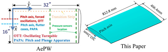
Figure 11.
BSCW geometry.
Table 3.
The structural data of the BSCW model.
3.2.1. Structural Finite Element Model
To ensure consistency with the structural data in reference [42], the plate finite element model (plate FEM) consisting of eight quadrilateral elements with fifteen grid points was employed to emulate the structural dynamic characteristics. The finite element model for the BSCW wing shape (shape FEM) without the material density property was also adopted. The plate FEM and the shape FEM were combined using multipoint constraints to form the overall FEM (Figure 12). To match the wing’s total pitch inertia, a concentrated inertia was placed at the pitch rotational axis at the chord-wise center of the plate FEM. To match the total mass, the concentrated masses were equally distributed among fifteen grid points of the plate FEM. Figure 12 gives the node number, and “Node n” represents the node number. Node 16 was placed at the same location as Node 2. Node 16 was constrained to six degrees of freedom (fixed condition). Node 2 and Node 16 were connected by a multipoint constraint, which constrained them to four degrees of freedom, allowing only movement through lift–directional translation and moment–directional rotation. The linear and torsional springs were set between Node 16 and Node 2. These two spring stiffnesses are shown in Table 3. Figure 12 shows a detailed description of the FEM of the BSCW. The blue part is the BSCW wing shape FEM, the orange part is the plate FEM, and the green part is the overall FEM.

Figure 12.
The BSCW finite element model.
The natural frequencies and normal modes of the plate FEM and the overall FEM were separately analyzed using the reduced solution of the equation of motion () without considering the damping and external force. The real eigenvalues were extracted using the Lanczos method, which combines the best characteristics of both the tracking and transformation methods. After comparison, the natural frequencies and normal modes were consistent. Figure 13 shows the modes of the plate FEM and the overall FEM. Table 4 gives the comparison frequencies of the overall model and relevant reference data. The overall FEM was used for the subsequent IDA analysis.

Figure 13.
The structural dynamic mode shapes of the BSCW.
Table 4.
The natural frequencies of the BSCW model.
3.2.2. Aerodynamic Finite Volume Model
To compute the unsteady aerodynamic forces, two types of structured fluid grids with different numbers of nodes were established (Figure 14). The medium grid had 425,450 cells and 40,976 nodes, and the fine grid had 1,913,818 cells and 1,870,272 nodes. The unsteady aerodynamic forces were calculated using the Spalart–Allmaras model.

Figure 14.
The aerodynamic model of the BSCW. (a) The medium grid with 40,976 nodes; (b) the fine grid with 1,870,272 nodes.
According to the BSCW wind tunnel data, the Mach number was 0.74, the dynamic pressure was 168 psf, the angle of attack was 0 deg, and the Reynolds number was million. These wind tunnel data were obtained in R12 gas, so R12 gas was also adopted in the CFD calculation. Table 5 gives the detailed aerodynamic input parameters after the unit conversion. It should be noted that the SI unit system was used in the aerodynamic analysis, the SI-mm unit system was used in the structural analysis process, and a unit conversion was performed to transform the data for the flutter analysis.
Table 5.
The R12 aerodynamic data.
First, the steady flow characteristics were obtained by solving the Navier–Stokes equations, which were then used as an initial solution for the coupled aeroelastic analysis. The pressure coefficients at 60% and 95% of the wing span were obtained to compare with the wind tunnel data. Figure 15 shows the pressure coefficients, and Figure 16 shows the dynamic pressure cloud. The pressure coefficients of both the medium and fine grid are consistent with the wind tunnel test results.
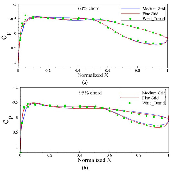
Figure 15.
A comparison of the static pressure coefficients: (a) 60% chord; (b) 95% chord.

Figure 16.
The static pressure coefficient of the BSCW.
Second, the medium and fine grids were used for the parametric analysis. The lift coefficients for different angles of attack were computed. In Figure 17, the right diagram gives the iterative convergence results of different AOAs, and the left diagram compares the results with those in reference [43]. After stalling, the accuracy of the aerodynamic calculations can be ensured using appropriate turbulence models (Spalart–Allmaras).

Figure 17.
The aerodynamic characteristics of the BSCW. (a) The lift coefficient (); (b) the iterative results of on the fine grid; (c) the moment coefficient (); (d) the iterative results of on the fine grid.
All these aerodynamic data confirm the reliability of the steady flow field calculation, thereby laying a good foundation for the subsequent flutter analysis. This foundation is crucial for the flutter analysis, and the accuracy of these initial calculations will influence the effectiveness of the IDA.
3.2.3. Flutter Results
In this paper, aeroelastic response curves were calculated for different dynamic pressures. The resulting flutter onset, as seen in Figure 18, occurred at a dynamic pressure of 7500 Pa, which is 7.20% below the experimentally measured onset dynamic pressure of 8082 Pa. A digital processing tool named ZARMA (short for ZONA’s ARMA), which belongs to ZONA Technology, Incorporated, was used to calculate the vibration frequency and damping. ARMA stands for auto-regressive moving average, which is a technique used to extract frequency and damping values from a given input signal. Figure 19 shows the frequency and damping curves at different dynamic pressures. When the dynamic pressure is 7500 Pa, the damping value is 0.0009, which is very close to zero. It can, thus, be concluded that the flutter’s critical dynamic pressure is 7500 Pa. The result of the frequency response curve indicates that the flutter frequency is 4.1 Hz. In order to verify the influence of the time step, the aeroelastic response calculations of different time steps were carried out. The response calculation results at three step sizes are given in Figure 20. According to the picture, it can be analyzed that the calculation results converge as the time step decreases, and the time step has little effect on the results.

Figure 18.
The BSCW flutter results (medium grid). (a) Time–displacement response curves; (b) frequency response curve (q = 7500 Pa).

Figure 19.
Frequency and damping coefficient vs. dynamic pressure. (a) Frequency; (b) damping coefficient.

Figure 20.
The results of different time steps at a dynamic pressure of 7500 Pa.
To examine the grid independence, the fine grid was used to compute the result for Pa. Figure 21 shows that the fine grid and medium grid results are consistent. The damping calculated using ZARMA for the fine grid was −0.0053, which is less than zero. If the dynamic pressure continued to increase, the damping would eventually exceed zero, so the fine grid more closely matches the wind tunnel result. Table 6 lists the IDA and wind tunnel results. The NASA Langley Research Center developed an unstructured grid Reynolds-averaged Navier–Stokes solver, named FUN3D. Using this method, reference [43] gave that the resulting flutter onset occurred at a dynamic pressure of 7278 Pa (152 psf), and the vibration frequency was 4.2 Hz at the flutter’s onset. By a comparison with the calculation results of FUN3D, it can be clearly seen that the calculation results of this method are more accurate.

Figure 21.
The medium-grid and fine-grid results at a dynamic pressure of 7500 Pa. (a) Time–displacement response curve; (b) frequency response curve.
Table 6.
A comparison of the IDA results and wind tunnel data.
An innovative aeroelastic solution method was developed in this paper, which was the CFD/IDA-coupling method. The two-dimensional wing and the BSCW model were used to substantiate the credibility. The CFD/IDA-coupling method demonstrated significant innovation within the field of aeroelastic simulations. Figure 20 and Figure 21 show that this method has good stability. Meanwhile, compared with the existing coupling approaches in the literature, the CFD/IDA-coupling method has good computational accuracy (see Table 6). In summary, its novelty is primarily reflected in two aspects. On the one hand, it has good stability. Under complex flow conditions, existing methods often struggle to maintain stability. The IDA framework enhances numerical stability under these conditions through improved coupling strategies and the Newmark- method, thereby increasing the reliability of the simulation results. On the other hand, it can increase the simulation accuracy. The IDA framework uses more refined meshing and more accurate physical models, thereby improving the simulation accuracy of complex aeroelastic phenomena.
4. Conclusions
This paper has presented a novel aeroelastic solution methodology, named the implicit dynamic approach (IDA), and explained its theoretical derivation. Central to the IDA is the application of the Navier–Stokes equations to resolve unsteady aerodynamic forces essential for aeroelasticity studies. A time-step-coupling data-solving interface was developed to bridge the structural and fluid dynamic domains for integrated aeroelastic analyses. A two-dimensional wing and the benchmark supercritical wing (BSCW) were used to analyze the aeroelastic response. The IDA’s flutter results for the two-dimensional wing were compared with those from the frequency domain method, and the IDA’s flutter results of the BSCW were compared with the wind tunnel data. All these comparison results show that the IDA’s calculation results are reliable. In conclusion, the credibility and stability of the IDA have been validated through analyses of a two-dimensional wing and the BSCW, demonstrating its reliability in predicting aeroelastic responses. The IDA stands as a powerful tool for aeroelastic problem analysis, and with further refinement, it is poised to significantly impact the fields of aeroelastic analysis and design.
Author Contributions
Conceptualization, W.Q. and W.W.; methodology, W.W.; software, W.W. and Z.C.; validation, X.A. and Z.C.; formal analysis, W.W.; investigation, W.W., X.A. and Z.C.; resources, W.W.; data curation, W.W.; writing—original draft preparation, W.W.; writing—review and editing, W.W. and X.A.; visualization, W.W. and Z.C. All authors have read and agreed to the published version of the manuscript.
Funding
This research received no external funding.
Data Availability Statement
Data is contained within the article.
Conflicts of Interest
The authors declare no conflicts of interest.
Abbreviations
The following abbreviations are used in this manuscript:
| CFD | Computational fluid dynamics |
| CSD | Computational structural dynamics |
| IDA | Implicit dynamic approach |
| BSCW | Benchmark supercritical wing |
References
- Hassig, H.J. An Approximate True Damping Solution of the Flutter Equation by Determinant Iteration. J. Aircraft. 1971, 8, 885–889. [Google Scholar] [CrossRef]
- Gu, Y.S.; Yang, Z.C. Modified p-k Method for Flutter Solution with Damping Iteration. AIAA J. 2012, 50, 507–510. [Google Scholar] [CrossRef]
- Chen, P.C. Damping Perturbation Method for Flutter Solution: The g-Method. AIAA J. 2000, 38, 1519–1524. [Google Scholar] [CrossRef]
- Rodden, W.P.; Giesing, J.P.; Kalman, T.P. Refinement of the nonplanar aspects of the subsonic doublet-lattice lifting surface method. J. Aircraft. 1972, 9, 69–73. [Google Scholar] [CrossRef]
- Guruswamy, G.P. Perspective on CFD/CSD-Based Computational Aeroelasticity during 1977–2020. J. Aerosp. Eng. 2021, 34, 06021005. [Google Scholar] [CrossRef]
- Hou, H.S.; Luo, C.; Zhang, H.; Wu, G.C. Frequency domain approach to the critical step size of discrete-time recurrent neural networks. Nonlinear Dyn. 2023, 111, 8467–8476. [Google Scholar] [CrossRef]
- Bosch, A.; Schmehl, R.; Tiso, P.; Rixen, D. Dynamic Nonlinear Aeroelastic Model of a Kite for Power Generation. J. Guid. Control. Dynam. 2014, 37, 1426–1436. [Google Scholar] [CrossRef]
- Brüderlin, M.; Hosters, N.; Behr, M. Robust Active Control of a Winglet with Elastic Suspension at Transonic Flow. J. Guid. Control. Dynam. 2018, 41, 526–534. [Google Scholar] [CrossRef]
- Smith, M.J. Conservation Issues for Reynolds-Averaged Navier–Stokes-Based Rotor Aeroelastic Simulations. J. Aerosp. Eng. 2012, 25, 217–227. [Google Scholar] [CrossRef]
- Zhang, J.A.; Shotorban, B.; Zhang, S. Numerical Experiment of Aeroelastic Stability for a Rocket Nozzle. J. Aerosp. Eng. 2017, 30, 04017041. [Google Scholar] [CrossRef]
- Wang, T.S.; Zhao, X.; Zhang, S.; Chen, Y.S. Development of an Aeroelastic Modeling Capability for Transient Nozzle Flow Analysis. J. Propul. Power. 2014, 30, 1692–1700. [Google Scholar] [CrossRef]
- De Castro, A.; Lee, H.; Wiecek, M.M. A Lagrange multiplier method for fluid-structure interaction: Well-posedness and domain decomposition. Comput. Math. Appl. 2025, 181, 193–215. [Google Scholar] [CrossRef]
- Zhang, W.; Jiang, Y.; Ye, Z. Two better loosely coupled solution algorithms of CFD based aeroelsatic simulation. Eng. Appl. Comp. Fluid 2007, 1, 253–262. [Google Scholar] [CrossRef][Green Version]
- Liu, W.; Huang, C.; Yang, G. Time efficient aeroelastic simulations based on radial basis functions. J. Comput. Phys. 2017, 330, 810–827. [Google Scholar] [CrossRef]
- Xie, L.; Xu, M.; Cai, T. Flutter and dynamic analysis based on CFD/CSD coupling method. J. Vib. Shock 2012, 31, 106–110. [Google Scholar] [CrossRef]
- Yang, J.; Zhang, W.W. Forced Response Analysis of Rotor Blades with the Mode-Based Aeroelastic Model. J. Aerosp. Eng. 2025, 38, 04025010. [Google Scholar] [CrossRef]
- Huang, G.; Dai, Y.; Yang, C.; Huang, C.; Zou, X. Gust Energy Harvesting of a Free-Flying Aircraft Model by CFD/CSD Simulation and Wind Tunnel Testing. J. Aerosp. Eng. 2022, 35, 04021105. [Google Scholar] [CrossRef]
- Naseri, A.; Lehmkuhl, O.; Gonzalez, I.; Bartrons, E.; Pérez-Segarra, C.D.; Oliva, A. A semi-implicit coupling technique for fluid–structureinteraction problems with strong added-mass effect. J. Fluid Struct. 2018, 80, 94–112. [Google Scholar] [CrossRef]
- Vindignia, C.R.; Mantegnaa, G.; Orlandoa, C.; Alaimoa, A.; Berci, M. A refined aeroelastic beam finite element for the stability analysis of flexible subsonic wings. Comput. Struct. 2025, 307, 107618. [Google Scholar] [CrossRef]
- Mozaffari-Jovin, S.; Firouz-Abadi, R.D.; Roshanian, J. Flutter of wings involving a locally distributed flexible control surface. J. Sound. Vib. 2015, 357, 377–408. [Google Scholar] [CrossRef]
- Huang, C.; Huang, J.; Song, X.; Zheng, G.; Nie, X. Aeroelastic Simulation Using CFD/CSD Coupling Based on Precise Integration Method. Int. J. Aeronaut. Space Sci. 2020, 21, 750–767. [Google Scholar] [CrossRef]
- Dai, H.; Yue, X.; Yuan, J.; Xie, D.; Atluri, S.N. A comparison of classical Runge-Kutta and Henon’s methods for capturing chaos and chaotic transients in an aeroelastic system with freeplay nonlinearity. Nonlinear Dynam. 2015, 81, 169–188. [Google Scholar] [CrossRef]
- Sha, D.S.; Tamma, K.; Li, M.C. A linear complementary based implicit dynamic approach for frictional contact-impact problems with elasto-plastic large deformation. In Proceedings of the 36th Structures, Structural Dynamics and Materials Conference, AIAA, New Orleans, LA, USA, 10 April 1995; pp. 246–247. [Google Scholar]
- Lavrenčič, M.; Brank, B. Simulation of shell buckling by implicit dynamics and numerically dissipative schemes. Thin Wall Struct. 2018, 132, 682–699. [Google Scholar] [CrossRef]
- Lavrenčič, M.; Brank, B. Hybrid-Mixed Shell Finite Elements and Implicit Dynamic Schemes for Shell Post-buckling. In Recent Developments in the Theory of Shells; Altenbach, H., Chróścielewski, J., Eremeyev, V.A., Wiśniewski, K., Eds.; Springer International Publishing: Cham, Switzerland, 2019; pp. 383–412. [Google Scholar] [CrossRef]
- Tian, Q.Q.; Yang, X.H.; Zhang, H.X.; Xu, D. An implicit robust numerical scheme with graded meshes for the modified Burgers model with nonlocal dynamic properties. Comput. Appl. Math. 2023, 42, 682–699. [Google Scholar] [CrossRef]
- Marino, E.; Kiendl, J.; De Lorenzis, L. Isogeometric collocation for implicit dynamics of three-dimensional beams undergoing finite motions. Comput. Methods Appl. Mech. Eng. 2019, 356, 548–570. [Google Scholar] [CrossRef]
- Maliska, C.R. Fundamentals of Computational Fluid Dynamics: The Finite Volume Method; Springer International Publishing AG: Cham, Switzerland, 2023; pp. 15–31. [Google Scholar] [CrossRef]
- Moioli, M.; Breitsamter, C.; Sørensen-Libik, K. Spalart-Allmaras Turbulence Model Conditioning for Leading-Edge Vortex Flows. In Advanced Aircraft Understanding Via the Virtual Aircraft Model; Heinrich, R., Ed.; Springer International Publishing AG: Cham, Switzerland, 2024; pp. 129–135. [Google Scholar] [CrossRef]
- Balakrishnan, A. Aeroelasticity: The Continuum Theory; Springer: New York, NY, USA, 2012; pp. 269–323. [Google Scholar] [CrossRef]
- Sinha, R. Advanced Newtonian Rigid Dynamics; Springer: Singapore, 2023; pp. 127–248. [Google Scholar] [CrossRef]
- Benacquista, M.J.; Romano, J.D. Classical Mechanics; Springer International Publishing AG: Cham, Switzerland, 2018; pp. 49–51. [Google Scholar] [CrossRef]
- Hilber, H.M.; Hughes, T.J.R.; Taylor, R.L. Improved numerical dissipation for time integration algorithms in structural dynamics. Earthq. Eng. Struct. Dyn. 1977, 5, 283–292. [Google Scholar] [CrossRef]
- Hou, G.; Wang, J.; Layton, A. Numerical Methods for Fluid-Structure Interaction—A Review. Commun. Comput. Phys. 2012, 12, 337–377. [Google Scholar] [CrossRef]
- Hu, Z.; He, S.; Lu, B.; Zha, J. A Study on the Two-Dimensional Numerical Simulation of Wing Flutter in a Heavy Gas. Aerospace 2025, 12, 247. [Google Scholar] [CrossRef]
- Vindigni, C.R.; Esposito, A.; Orlando, C. Stochastic aeroservoelastic analysis of a flapped airfoil. Aerosp. Sci. Technol. 2022, 131, 107967. [Google Scholar] [CrossRef]
- Mozaffari-Jovin, S.; Firouz-Abadi, R.D.; Roshanian, J. L1 adaptive aeroelastic control of an unsteady flapped airfoil in the presence of unmatched nonlinear uncertainties. J. Sound. Vib. 2024, 578, 118334. [Google Scholar] [CrossRef]
- Heeg, J.; Chwalowski, P.; Florance, J.P.; Wieseman, C.D.; Schuster, D.M.; III, B.P. Overview of the Aeroelastic Prediction Workshop. In Proceedings of the 51st AIAA Aerospace Sciences Meeting Including the New Horizons Forum and Aerospace Exposition, Grapevine, TX, USA, 7–10 January 2013; pp. 5–8. [Google Scholar] [CrossRef]
- Heeg, J.; Chwalowski, P.; Schuster, D. Overview and Lessons Learned from the Aeroelastic Prediction Workshop. In Proceedings of the 54th AIAA/ASME/ASCE/AHS/ASC Structures, Structural Dynamics, and Materials Conference, Boston, MA, USA, 8–11 April 2013; pp. 1–7. [Google Scholar] [CrossRef]
- Heeg, J.; Wieseman, C.D.; Chwalowski, P. Data comparisons and summary of the second AIAA Aeroelastic Prediction Workshop. In Proceedings of the 34th AIAA Applied Aerodynamics Conference, Washington, DC, USA, 13–17 June 2016; pp. 1–32. [Google Scholar] [CrossRef]
- Chwalowski, P.; Stanford, B.; Jacobson, K.; Poplingher, L.; Raveh, D.E.; Jirasek, A.; Pagliuca, G.; Marcello, R. Flutter Prediction Report in Support of the High-Angle Working Group at the Third Aeroelastic Prediction Workshop. In Proceedings of the AIAA SCITECH 2024 Forum, Orlando, FL, USA, 8–12 January 2024; pp. 1–18. [Google Scholar] [CrossRef]
- Heeg, J.; Chwalowski, P.; Schuster, D.M.; Raveh, D.; Jirasek, A.; Dalenbring, M. Plans and Example Results for the 2nd AIAA AeroelasticPrediction Workshop. In Proceedings of the 56th AIAA/ASCE/AHS/ASC Structures, Structural Dynamics, and Materials Conference, Kissimmee, FL, USA, 5–9 January 2015; pp. 7–9. [Google Scholar] [CrossRef]
- Heeg, J.; Chwalowski, P. Investigating the Transonic Flutter Boundary of the Benchmark Supercritical Wing. In Proceedings of the 58th AIAA/ASCE/AHS/ASC Structures, Structural Dynamics, and Materials Conference, Grapevine, TX, USA, 7–10 January 2017; p. 10. [Google Scholar] [CrossRef]


Disclaimer/Publisher’s Note: The statements, opinions and data contained in all publications are solely those of the individual author(s) and contributor(s) and not of MDPI and/or the editor(s). MDPI and/or the editor(s) disclaim responsibility for any injury to people or property resulting from any ideas, methods, instructions or products referred to in the content. |
© 2025 by the authors. Licensee MDPI, Basel, Switzerland. This article is an open access article distributed under the terms and conditions of the Creative Commons Attribution (CC BY) license (https://creativecommons.org/licenses/by/4.0/).