1. Introduction
Autonomous positioning has been a topic of research for many years [
1], but its implementation has proven more complicated than autonomous attitude determination. As missions become more complex, it is desirable for a spacecraft to be able to estimate its position independently from ground, if not all of the time, at least as a back up in case of a loss of communication, either accidental or foreseen. In particular, spacecraft orbiting or en route to a satellite or a planet other than the Earth are periodically out of line-of-sight from any ground station and, thus, have to rely on their on-board capabilities. Utilizing pre-existing sensors to obtain a navigation solution is an attractive solution to the backup autonomous navigation problem. Among those, optical cameras have been a mainstay of spacecraft sensor arrays since the beginning of space exploration. The availability of onboard cameras, together with the advancement of the fields of image processing and feature identification, has led to the proposed approach of an algorithm for autonomous spacecraft positioning via analysis of optical images of a reflective celestial body in the proximity of the spacecraft itself.
The first optical navigation approaches used cameras to take pictures of target illuminated bodies against a background of cataloged reference stars. This technique was first proposed in the 1960s (see [
2]). This approach was then adopted in six Voyager flybys of the outer planets [
3,
4] and Cassini’s orbital operations at Saturn [
5]. In particular, for the Voyager II Uranus approach and encounter, [
3,
4] presented the optical observables. These observables were based on measuring the angular distances between stars and the observed body (considered as a circle) and require the use of two cameras. The approach proposed in this paper uses a single camera and does not use observed stars. The main reason is the optimal observation of stars and illuminated bodies is associated with different exposures (integration time). To observe stars and bodies, two cameras are needed.
The work in [
6] adopts the Canny edge detection algorithm to identify the Moon edges. Then, the potential false edges are removed, and the limb profile is identified by the Levenberg–Marquardt ellipse least-squares algorithm. The line-of-sight (LOS) vector to the centroid of the observed object is then obtained. The approach taken in this study is different and optimized for use in small on-board computers. More accurate edge detection algorithms and optimization techniques are certainly available in the literature. Many alternative approaches to better select contours (hard edge pixels) do exist. Laplacian, Sobel, Roberts and Prewitt operators, as well as Gaussian derivatives and Gabor filters are certainly more accurate (while computationally more intensive) than the proposed simple numerical gradient, and an extensive literature exists on the comparison subject. Pushing the accuracy to select better pixels has been analyzed, and it has been found unnecessary, because the final accuracy (what really matters) is provided by the results of nonlinear least-squares estimation using circular sigmoid functions. To avoid computationally-intensive approaches, simple image differentiation is here adopted to select the pixels of interest. Using these pixels, accurate Moon radius and centroid are estimated by a fast nonlinear least-squares using circular sigmoid functions.
The works in [
7,
8] contain a thorough comparison analysis between various different mathematical approaches to perform the best fitting of circles and ellipses. While this study deals with the same problem, it does not follow the above approach for the following two reasons: (1) the image-plane ellipse eccentricity of the observed Moon is really small (almost negligible) for a typical imager; and (2) when the ellipse eccentricity is so small (as in our physical example), the least-squares estimation of the ellipse orientation (and the difference of the semi-axes) is unreliable (unobservable parameters). In this case, circle least-squares estimation is numerically more stable.
The pin-hole camera model performs gnomonic projection, and this projection introduces radial distortion. This means that the spherical Moon is observed as an ellipse. However, using the Aptina imager with a 0.0022-mm pixel size and 16-mm focal length (this allows one to observe the Moon for an entire cislunar trajectory), the worst radial distortion (the Moon is observed as far as possible from the optical axis) is less than one pixel. These (really small) radius and centroid corrections (due to this small radial distortion) are easy to implement. This correction depends on the specific imager adopted. The elliptical best fitting approach is discouraging because (for such small eccentricity) the ellipse orientation becomes unobservable. Analytical studies and extensive numerical tests are done to support the proposed approach.
This work refines a previous study [
9], focusing on the analysis of Moon images, both real and synthetic. However, the basic idea is applicable to any spherical reflective celestial body within relative proximity to the spacecraft. In this study, the Moon radius and centroid is estimated in two steps. First, Taubin’s technique [
10] has been adopted just to obtain a crude first estimation. This first estimation is then used to select the set of pixels between two radii across the Moon’s hard edge, and it is used (as the initial guess) for the subsequent accurate iterative nonlinear least-squares estimation approach using circular sigmoid functions. Circular sigmoid functions accurately describe the actual gray tone smooth transition at the hard edge. During this nonlinear least-squares, the smoothing parameter (
k) is also estimated.
The image processing approach is described in detail in the following sections. Further, several application examples are illustrated, together with an error analysis.
2. Concept
The starting point of the method is the realization that in an image taken by a spacecraft of a reflective celestial body, if the illumination conditions are right and the pointing appropriate, the target will figure prominently in the image, against a mostly black background. Therefore, processing the image with a gradient filter, pixels belonging to the hard edge have the highest magnitudes, which makes them easily identifiable. These points can then be best fitted to estimate the apparent target radius and center and, thus, the relative distance between observer and target. Several steps need to be taken to ensure that the data points are properly selected and that the best fitting is accurate enough. The proposed algorithm can be summarized as follows:
The geometrical illumination conditions and the expected size of the observed body are first computed. These data allow one to determine whether the target is sufficiently illuminated and of sufficient size to perform the estimation process.
The image differentiation is obtained with a fourth order Richardson extrapolation.
The pixels of the gradient image are sorted in descending mode. Eventual outliers present in this set, due to noise or background stars, are then eliminated by two sequential filters.
- −
The first filter validates an edge pixel based on eigenanalysis of a small gradient box around the pixel and by investigation of the same box in the original image.
- −
The second filter is a modified version of the RANSAC algorithm.
The edge points selected are then used to obtain the first estimate of center and radius. The Taubin best fitting algorithm [
10] is used.
The first estimate is refined via non-linear least-squares using a circular sigmoid function to describe the edge transition.
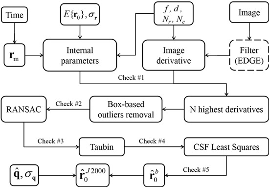
Required inputs to the image processing software are (see
Figure 1):
Camera: This includes focal length (f) in mm and imager data (number and size of rows and columns).
Image: This is the image (made of rows and columns) taken at the specified time.
Time: This is the time instant at which the image is taken. This time is used to compute the Moon and Sun positions in J2000.
Position: This input consists of a raw estimate of the spacecraft position, , and its accuracy, . These data are used to estimate the Moon’s radius on the imager and the expected illumination condition. This position estimate is very rough, having typical an accuracy of less than 10,000 km.
Attitude: This input consists of the spacecraft attitude, , and attitude accuracy, . These data are used to compute the spacecraft-to-Moon vector in the J2000 reference frame.
Figure 1.
Image processing general flowchart.
Figure 1.
Image processing general flowchart.
Input of the proposed approach are: (1) the time, (2) the camera focal length (f), (3) the pixel size (d), (4) the image, and (5) an rough estimation of the position () with it’s accuracy (). From time the inertial positions of Moon () and Sun () can be computed. Using the knowledge of the camera parameters and it is possible to derive important internal parameters, such as the expected Moon radius (in pixel) on the imager and the observed body illumination conditions. If the image is synthetic (e.g., generated by EDGE), then a simple convolution filter will smooth the image from pixellation. The image gradient is then generated using numerical differentiation and the N highest derivatives are selected (most of them belong to the Moon edge while a few are outliers due to the Moon topology). The outliers are then eliminated by two sequential filters, a box-based one followed by RANSAC. Once the outliers are eliminated a preliminary estimation of the Moon center and radius can be performed by least-squares using Taubin approach. Using this initial estimate, a set of pixels across the estimated Moon edge and angularly close to the Sun direction in the imager, are identified. These pixels are then used to obtain an accurate estimation of the Moon center and radius using circular sigmoid function as reference model. This allows us to estimate the vector to the Moon in the camera reference frame (). Finally, using the camera attitude () is then possible to compute the vector to the Moon in the inertial reference frame ().
The first check on the data is done using the rough expected value for the parameters, and the following section describes these calculations done for the Moon; however, they are applicable to any (almost) spherical celestial body. The following is based on geometric considerations alone and, thus, does not involve processing of the image data. This is why the parameters are described as “expected” values.
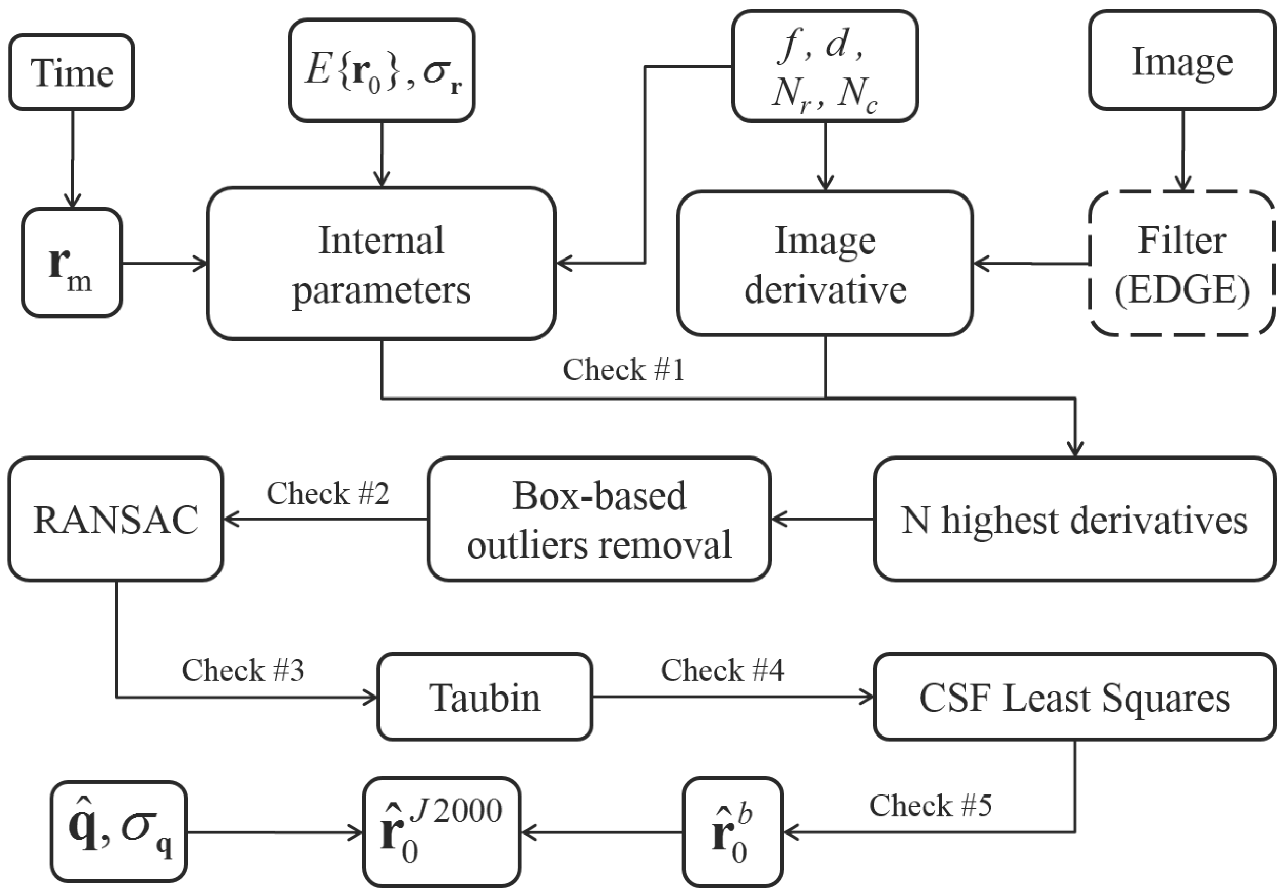
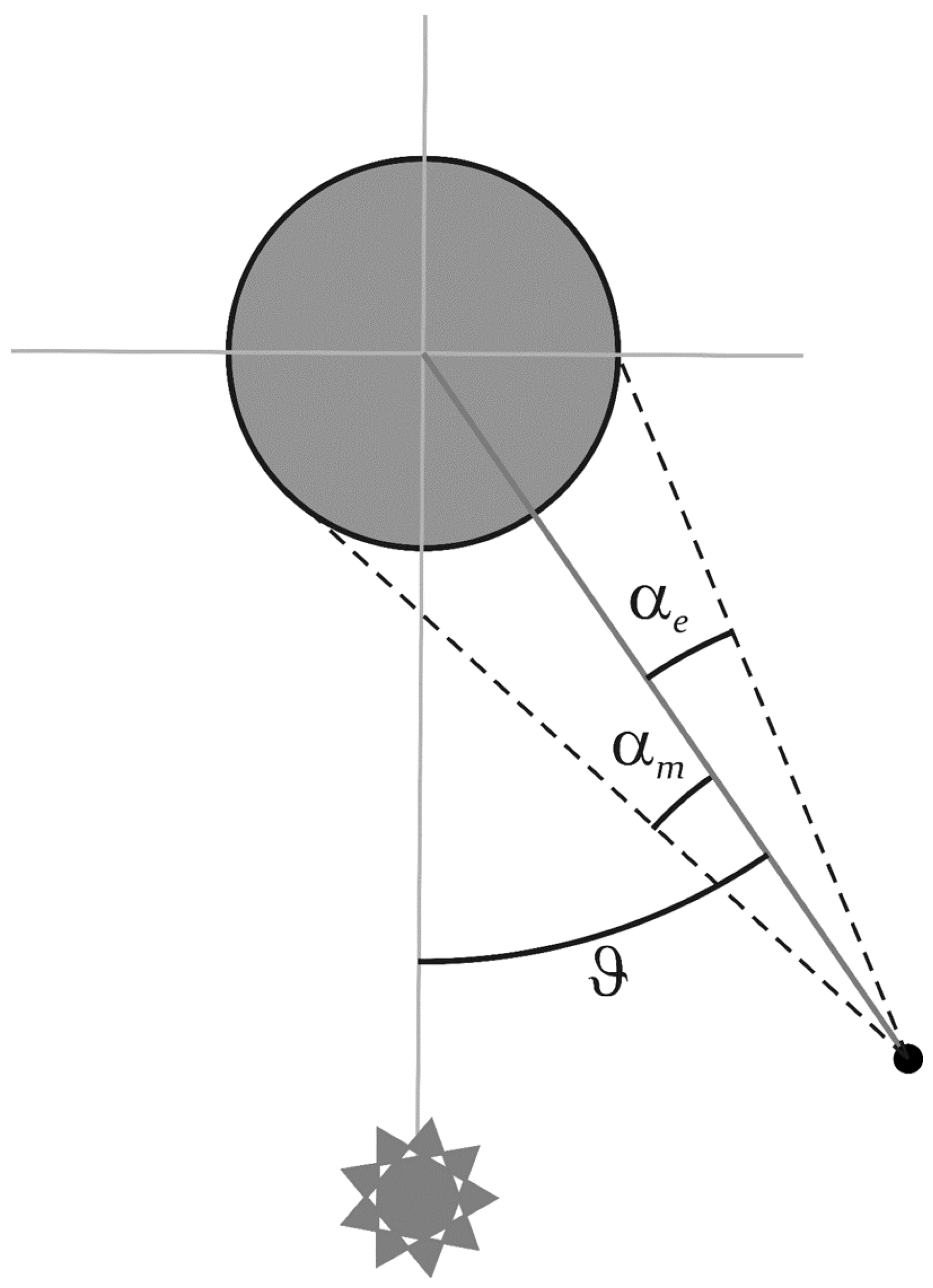
3. Expected Radius and Illumination Parameter
As the relative positions of observer, target and light source change, the visible part of the target varies. These changes can lead to cases in which the target is too thin or completely dark from the point of view of the observer, and therefore, no analysis can take place. The algorithm catches these degenerate cases before they can cause critical errors further down in the process. Two parameters are introduced to describe the target’s shape (from now on, for simplicity, the term “target” will refer just to the illuminated portion rather than the whole object, as this is what the camera is actually able to observe): one is the expected radius of the target
, and the other is the cross-length measured at its thickest point
(see
Figure 2), which is referred to as the illumination parameter. Both of these distances are measured in pixels, and they are estimated from the camera parameters (focal length
f, pixel size
d) and the observation geometry. For this purpose, the observer’s position is needed; however, even a high uncertainty (
10,000 km) has a very small impact on
and
, as long as the spacecraft is further from the target than a certain threshold. Such a rough position estimate can be considered known
a priori to start the analysis.
Figure 2.
Expected Moon radius () and illumination parameter ().
Figure 2.
Expected Moon radius () and illumination parameter ().
To begin, the expected radius and illumination angle are computed as:
where
is the Sun-to-Moon rays’ direction,
the observer-to-Moon vector and
the Moon radius. The expected radius is of great importance, not only because the illumination parameter is measured in relation to it, but also because it predicts the overall size of the target in the image, which is used in subsequent parts of the algorithm. The value of
is determined differently depending on the values of
and
ϑ.
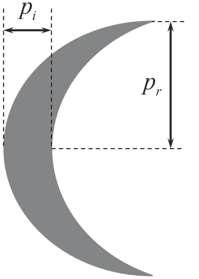
3.1. Full or New Moon
With reference to
Figure 3, the angle
can be derived from simple trigonometry:
This equation also allows one to define a critical distance,
, as the distance at which
:
Whether
is greater or smaller than
, together with the value of
ϑ, determines the case, according to the following scheme:
Figure 3.
Full/new Moon geometry.
Figure 3.
Full/new Moon geometry.
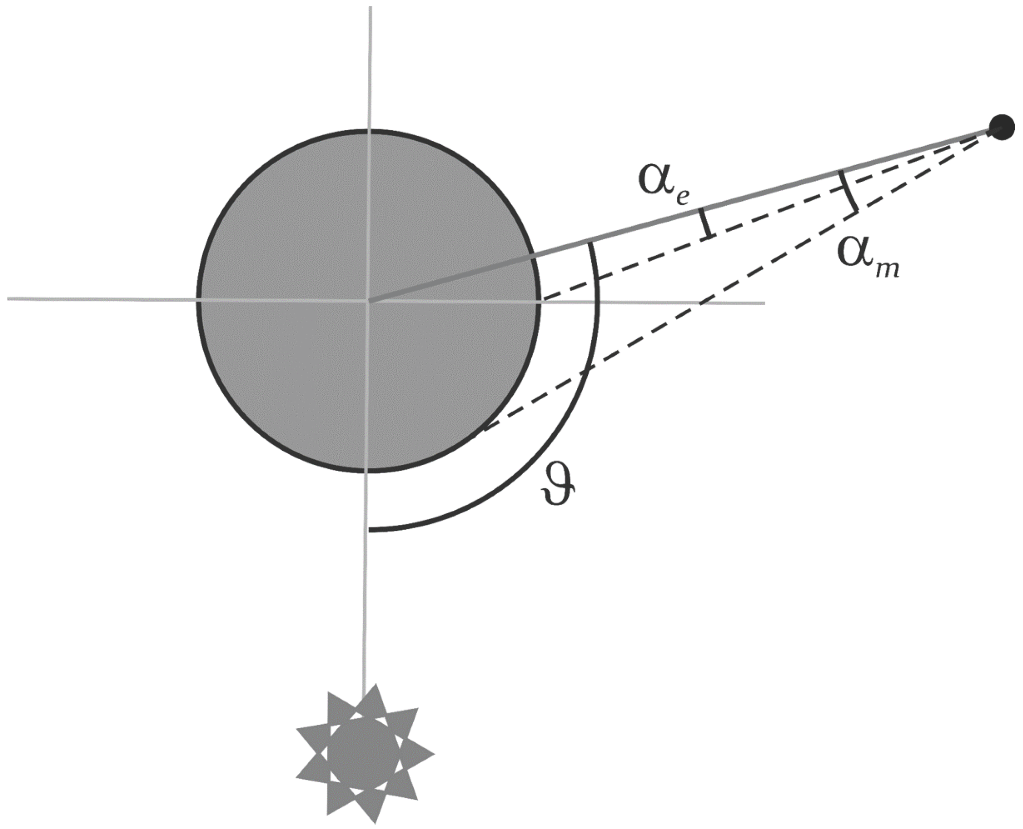
3.2. Gibbous Moon
The gibbous Moon occurs when:
For this configuration (see
Figure 4),
can be computed by finding the auxiliary variables
x and
:
which allows one to find the “excess” factor
:
and therefore,
Figure 4.
The gibbous Moon geometry.
Figure 4.
The gibbous Moon geometry.
3.3. Crescent Moon
The crescent Moon occurs when:
In this case (see
Figure 5), the two variables
x and
can be found according to:
and therefore:
Figure 5.
The crescent Moon geometry.
Figure 5.
The crescent Moon geometry.
Differentiating among these cases is important to properly initialize the algorithm. For this purpose, the analytical relations described above are supplemented with thresholds to ensure that the system works properly; for instance, when is lower than a certain value, the crescent is deemed too thin to be a reliable source of information, and the target is considered invisible.
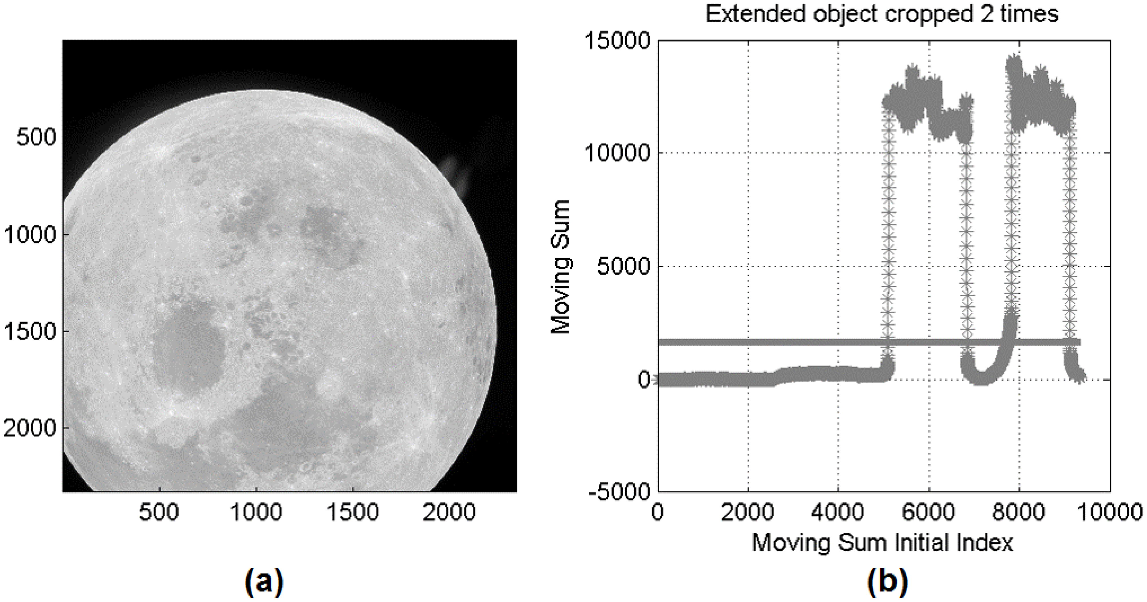
3.4. Special Case: Cropped Target
It is also possible for the target not to be completely within the field-of-view. The images’ boundaries are set with a rectangular mask proportional to the dimensions of the image itself. At each step, the cumulative brightness within the mask is computed and compared with a threshold value, for example a value tested to provide good performance is
of the maximum gray tone. From the amount of threshold crossings, it is possible to determine if and how many times the target has been cropped by the frame. An example application is depicted in
Figure 6.
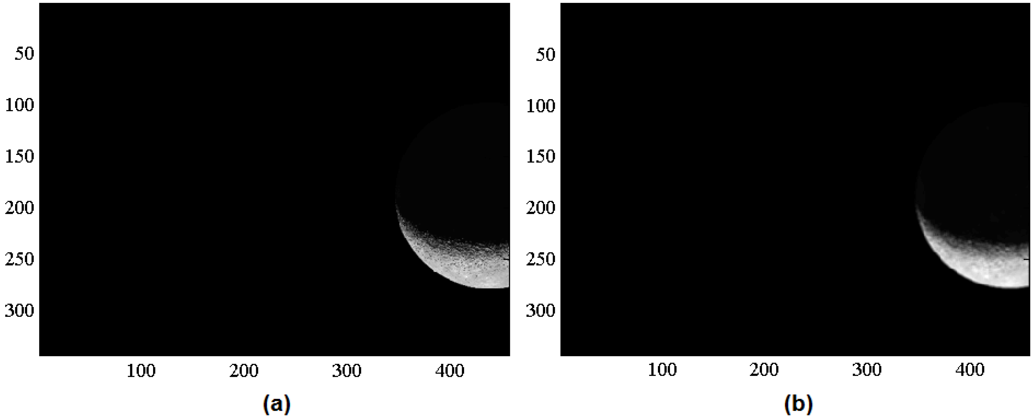
Figure 6.
Processing of a cropped image. (a) Cropped image of the Moon; (b) Results of the cropped detection.
Figure 6.
Processing of a cropped image. (a) Cropped image of the Moon; (b) Results of the cropped detection.
The values of
and
are used to initialize the following parameters:
Number of pixels in the gradient image to be analyzed (
N): This number has to be proportional to the length of the visible Moon arc. However, at this stage, it is impossible to know the angular width of the target; moreover, the presence of the terminator introduces a number of high contrast pixels that are not part of the Moon edge. Ultimately,
N is chosen to be proportional to
and
, according to the following:
where
k is a factor that varies linearly with
, from a minimum value (two) when
to a maximum equal to twice the minimum, when
.
The size of the box for box-based outliers removal (s): Because of the way the code works, the box has to be chosen small enough that the segment of the Moon edge within the box appears almost straight. Extensive testing has shown that the best choice is to take , with a lower limit of and an upper limit of .
RANSAC maximum distance: This is chosen equal to .
Number of tests for RANSAC (
): RANSAC randomly selects for testing a subset of all of the possible triplets of pixels remaining after the box-based outliers’ removal. Testing has shown that the best choice is to have:
where
is the number of selected pixels remaining after the box-based outliers’ filter rejection. The value of 500 is enforced as an upper limit.
Convergence tolerance for circular sigmoid function (CSF) least squares [
9]: At the
k-th iteration, the convergence check is performed on the solution variation
. Assuming the requirement accuracy is 0.3 pixel (in the center and radius estimation), the CSF-LS converge criteria is assumed to be 1/50 smaller than that,
.
The number of iterations for CSF least squares is .
As indicated in
Figure 1, several checks are implemented throughout the code. Failure to pass any of the tests causes the process to abort.
4. Gradient-Based Image Processing Algorithm
The gradient-based image processing approach is based on the expectation that the part of the image with the strongest variation of gray tones is the Moon’s observable hard edge. Pixels with the highest derivatives are the most likely to belong to the hard edge. However, the presence of bright stars, Moon surface roughness and other unexpected objects within the field-of-view creates several bright gradient pixels, which are not in fact part of the Moon hard edge. These points, called outliers, must therefore be eliminated from the dataset prior to using a best fitting algorithm to determine the sought geometrical properties. In this work, two separate outlier removal methods are implemented in sequence.
4.1. Image Differentiation
The gradient of the discrete gray tone function is computed by numerical differentiation; in particular, the gradient is computed using four-point central difference with a single Richardson extrapolation.
The row and column four-point central partial differences computed at pixel
are:
These derivatives are accurate with order
, where
h is the pixel dimension. The image gradient is then computed as:
A single Richardson extrapolation requires computing Equation (
19) one time with step
(getting
) and one time with step
h (getting
). Therefore, the true derivative can be written as:
Equating these two equations, we obtain:
and therefore:
An example of the application of a single Richardson extrapolation is done using the six-hump camel back function:
Using a single Richardson extrapolation a 4–5 orders of magnitude accuracy gain can be obtained. In this specific example, central two points and central four-points provide and level accuracy, respectively. However, when using Richardson extrapolation, central two-point and central four-point provide and level accuracy, respectively. Because it provides almost the machine error accuracy, the four-point central differentiation with Richardson extrapolation is selected to evaluate the image gradient.
The image gradient pixels are sorted by gradient value in descending mode, and the outliers are then eliminated with two methods discussed below.
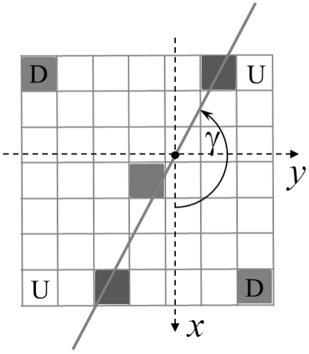
4.2. Box-Based Outlier Identification
The first approach is based on a local analysis around the pixel being considered as potentially belonging to the target’s edge. A mask like the one in
Figure 7, whose size depends on the parameter
, is centered on a candidate pixel. If the pixel does indeed belong to the target’s edge, then it is likely to be part of a sequence of pixels of comparable brightness distributed along a preferred direction. Moreover, the pixel should sit on the border between two areas where the gray tone “flattens” (the inside and outside of the target) and which therefore should appear as dark in the gradient image. If the pixel does not satisfy all of these conditions, it is rejected. To perform this analysis, first, the tensor of inertia of the gradient image within the mask is computed, and then, the eigenvectors and eigenvalues are found. The eigenvector associated with the minimum eigenvalue (continuous line direction in
Figure 7) is inclined by an angle
γ with respect to the row axis direction and represents the direction of the supposed edge.If
, then the farthest pixels from the edge line are those marked by “D”, while if
, the farthest pixels are those marked by “U”. Several conditions have to be satisfied for the pixel to be accepted:
The ratio between the eigenvalues must be lower than a certain threshold, chosen experimentally at . This indicates that the distribution of bright pixels has a preferential direction.
The values of the gradient in the pixels furthest from the edge line should be small, as both should be far from areas of variable brightness. Moreover, their gray tones should differ noticeably, as one belongs to the target and the other to the night sky.
For the pixels along the continuous line in
Figure 7, the ratio of their gradient values should be close to one (
), as they both supposedly belong to the edge.
For the pixels marked by “D” in the same figure, the ratio of their gray tone values should be close to zero (), as one belongs to the night sky and the other to the target.
Figure 7.
Mask for the box-based outlier identification technique (mask size: ).
Figure 7.
Mask for the box-based outlier identification technique (mask size: ).
4.3. RANSAC for Circle and Ellipse
The second technique is the standard RANSAC algorithm, which is an abbreviation for “random sample consensus” [
11]. It was developed for robust fitting of models in the presence of many data outliers. The algorithm is very simple and can be applied in the fitting of many geometric entities, such as lines, circles, ellipses,
etc. It is a non-deterministic iterative algorithm, in the sense that it produces a reasonable result only with a given probability, which increases as more iterations are allowed. It works by selecting random subsets of size equal to the number of unknown parameters and then checks whether the remaining data points lie further than a certain threshold from the curve determined by the initial subset. Repeating this process for many randomly-chosen subsets is likely to find and remove the outliers. More formally, given a fitting problem with
n data points and unknown
m parameters, starting with
, the classic RANSAC algorithm perform
times the following steps:
selects m data points at random;
finds the curve passing through these m points, thus estimating the associated m parameters;
counts how many data items are located at a distance greater than a minimum value from the curve; they are ;
if , then set .
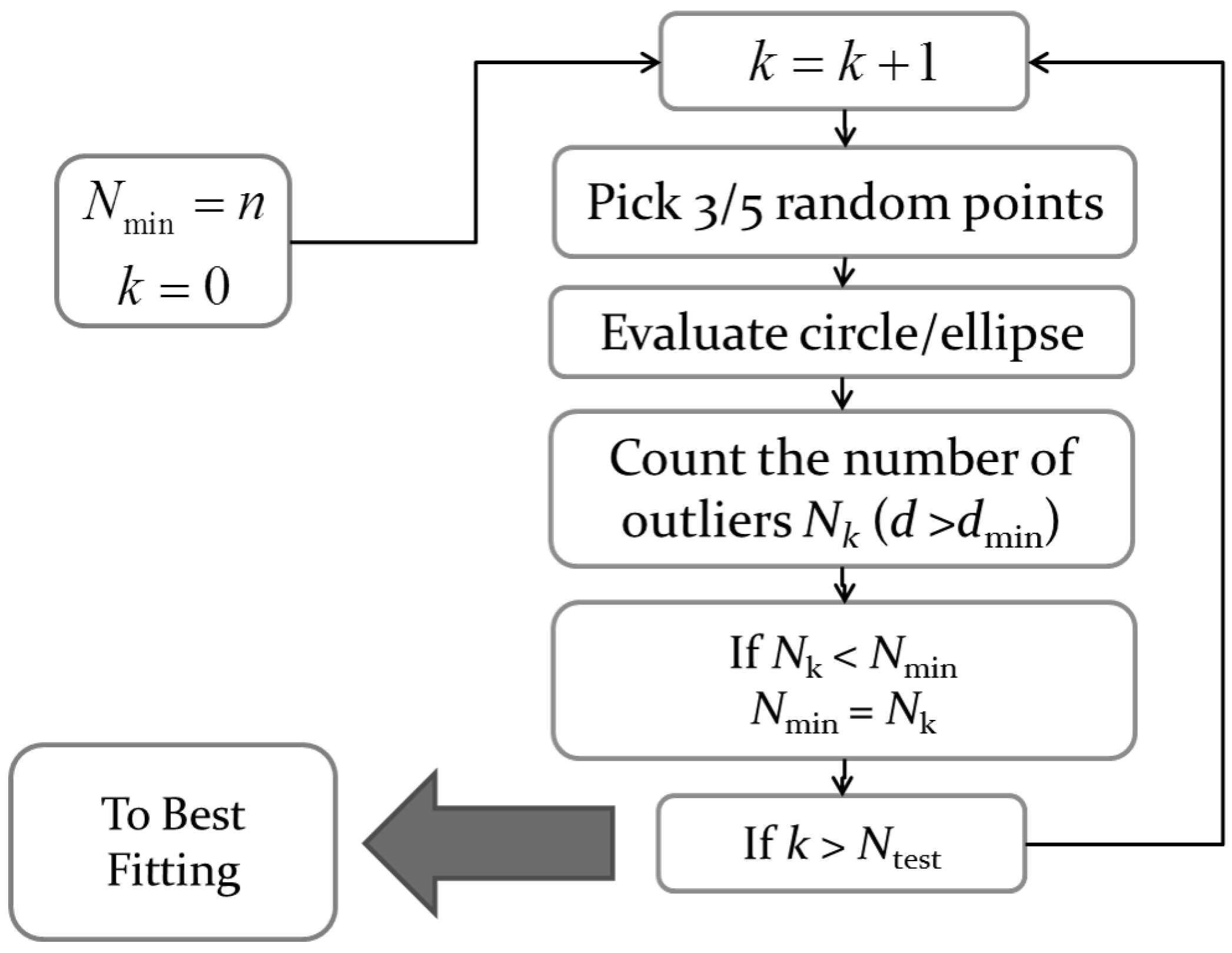
The basic cycle is depicted in
Figure 8.
Crucial to a successful implementation of RANSAC is the method used for the random selection of subsets. A purely random selection approach may persist in choosing outliers, with a great waste of computational time. On the other hand, a procedure based on deterministic inner loops can also be inefficient, if by chance, one outlier is selected by the outmost loop. Therefore, as an improvement of the basic method, a technique originally developed for pyramid star identification [
12] has been adopted, which always selects different subsets by continuously rotating the dataset indexes.
Figure 8.
RANSAC flowchart.
Figure 8.
RANSAC flowchart.
5. Circle Best Fitting
Once the pixels in the image have been selected, the algorithm determines the geometric characteristics of the observed body, that is apparent radius and center position within the image. The problem of recognizing geometrical entities and reducing them to a minimal set of parameters, sometimes called feature extraction, is very important in image processing for a number of applications in computer graphics and computer vision. Consequently, a great amount of research exists on developing methods to efficiently and unequivocally recognize geometrical shapes within an image; in particular, much literature is available regarding circle identification. Identifying geometrical figures within a discrete representation of the physical world reduces essentially to a best fitting problem. Currently, feature recognition techniques for conic curves fall within one of the following categories:
Geometric fit: Given a set of
n data points, iteratively converge to the minimum of:
where
are geometric distances from the data points to the conic and
x is the vector of the parameters to be found.
Algebraic fit:
are replaced with some other function of the parameters
, and thus, a new cost function is defined:
These functions typically are algebraic expression of the conic in question, which are usually simpler than the expression for geometric distances.
Historically, geometric fit has been regarded as being the more accurate of the two. However, this accuracy comes at the price of added computational cost and the possibility of divergence. Algebraic fit is typically reliable, simple and fast. A common practice is to use an algebraic fit to generate an initial guess for a subsequent iterative geometric fit, but in recent years, new algebraic fitting routines have shown such a degree of accuracy that geometric fits cannot improve it noticeably [
13].
5.1. Taubin Best Fitting
The following is a description of the Taubin best fitting method, first described in [
10], but using a formalism found in [
13]. This algorithm is used to obtain an initial estimate of the sigmoid best fitting algorithm. Given the circle implicit equation as:
the Taubin best fit minimizes the function:
which is equivalent to minimizing:
subject to the constraint:
where the bar sign indicates the simple average of the variables.
One important property of this method is that the results are independent of the reference frame. By reformulating this problem in matrix form, it becomes apparent how it is equivalent to a generalized eigenvalue problem. Indeed, define:
then the best fitting problem can be rewritten as:
where:
Therefore, the optimization problem is equivalent to the following generalized eigenvalue problem:
Since, for each solution,
:
then, to minimize
, the smallest positive eigenvalue is chosen. Because matrix
N has rank three, such an eigenvalue is found by explicitly solving the cubic characteristic equation without the necessity of implementing SVD or other computationally-intensive algorithms.
6. Numerical Tests
To support the capability of the developed image processing code, three numerical examples of a partially-observed Moon are presented here. All of these tests have been performed with no information about time, camera data and the observer, Moon and Sun positions. The image derivative is obtained using the four-point central approach with no Richardson extrapolation. This information clearly helps to define the best values of the internal parameters. Since this help is missing, the internal parameters have been adopted with the same values in all three tests. These values are:
Maximum number of highest derivatives selected: ;
Box-based outlier elimination: box size = ;
Box-based outlier elimination: derivative ratio ;
Box-based outlier elimination: corner ratio ;
Box-based outlier elimination: eigenvalue ratio ;
RANSAC: minimum distance pixels;
RANSAC: number of tests = 100.
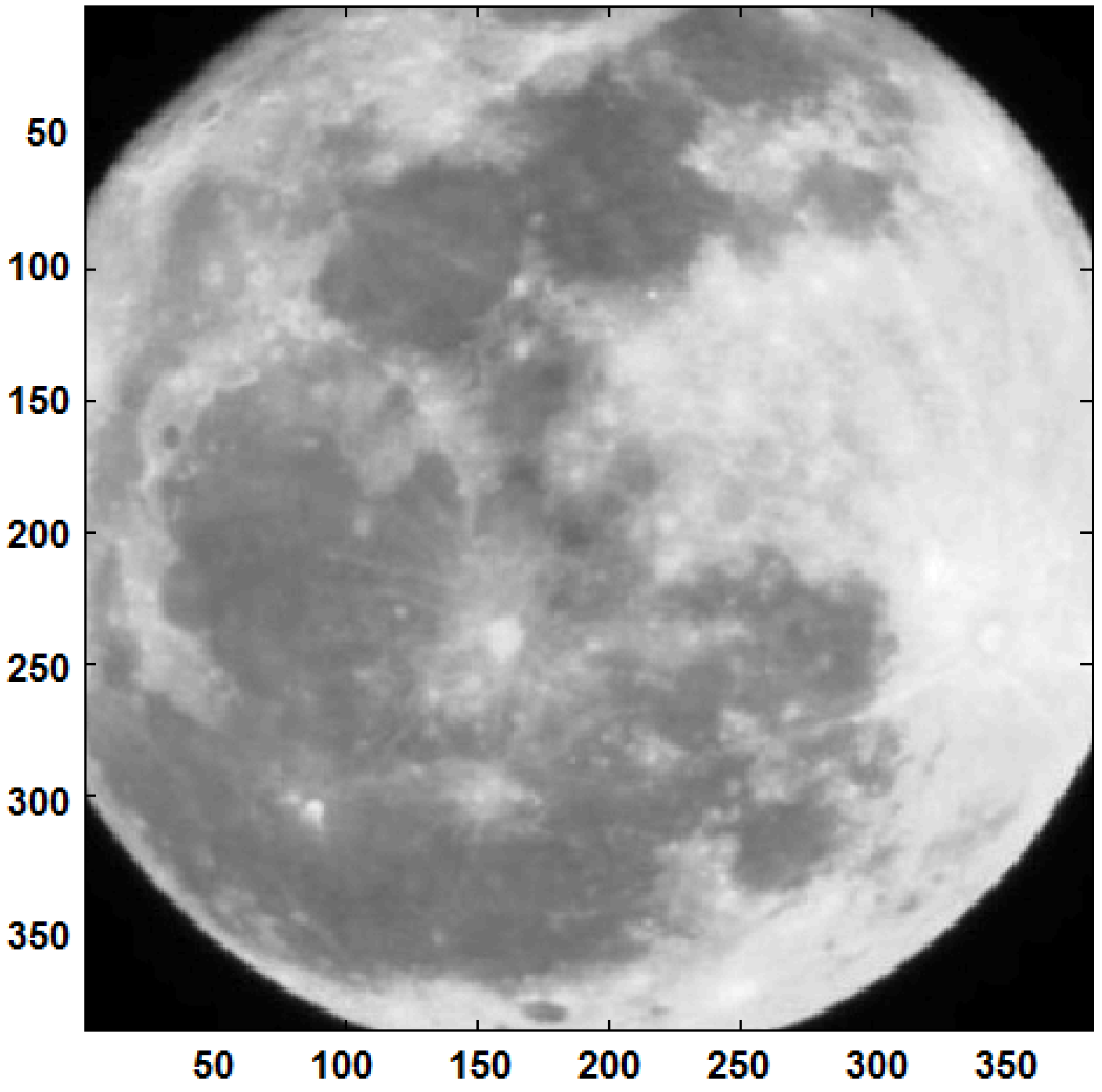
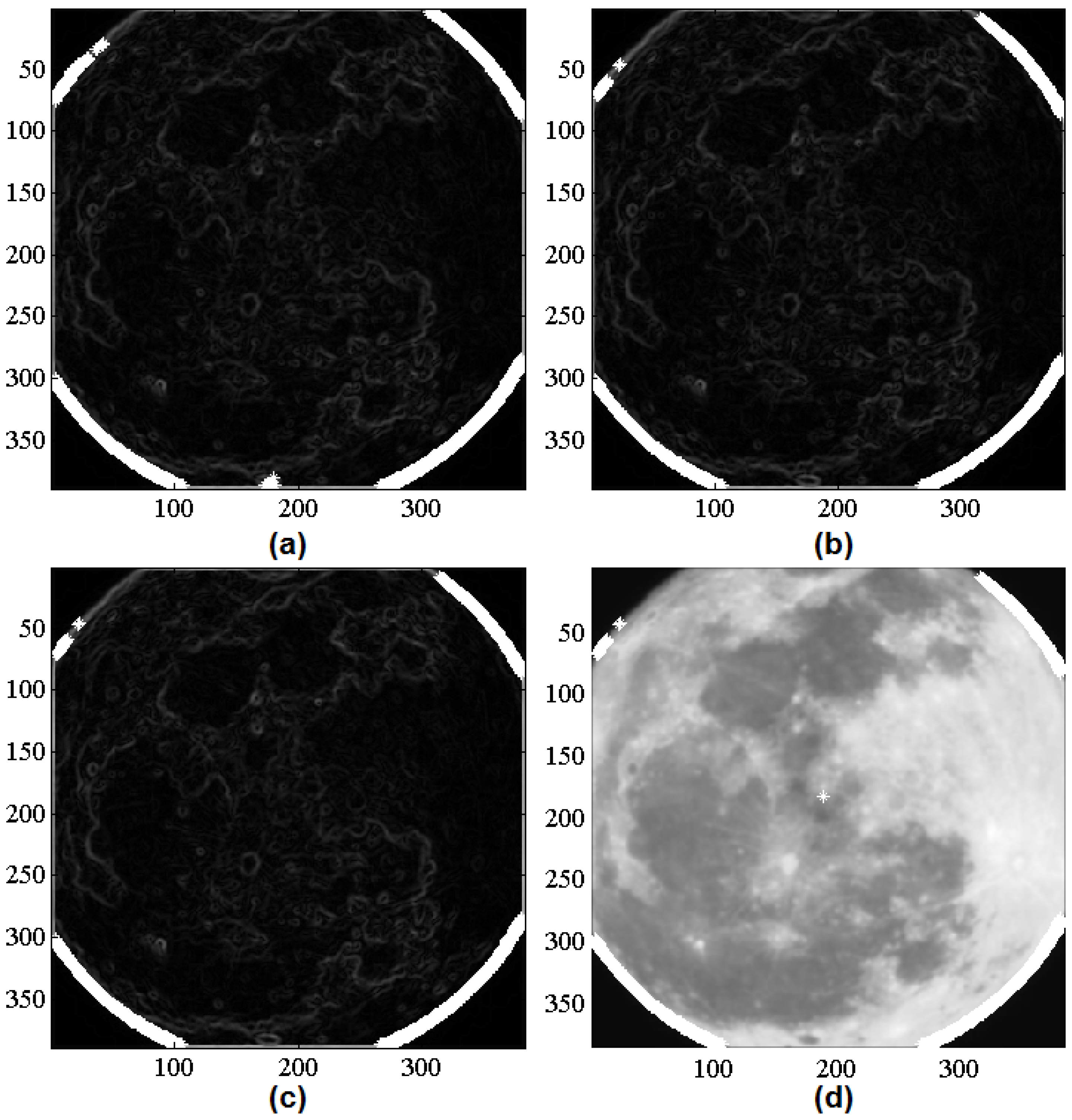
6.1. Example 1: Real Image, Four-Times Cropped
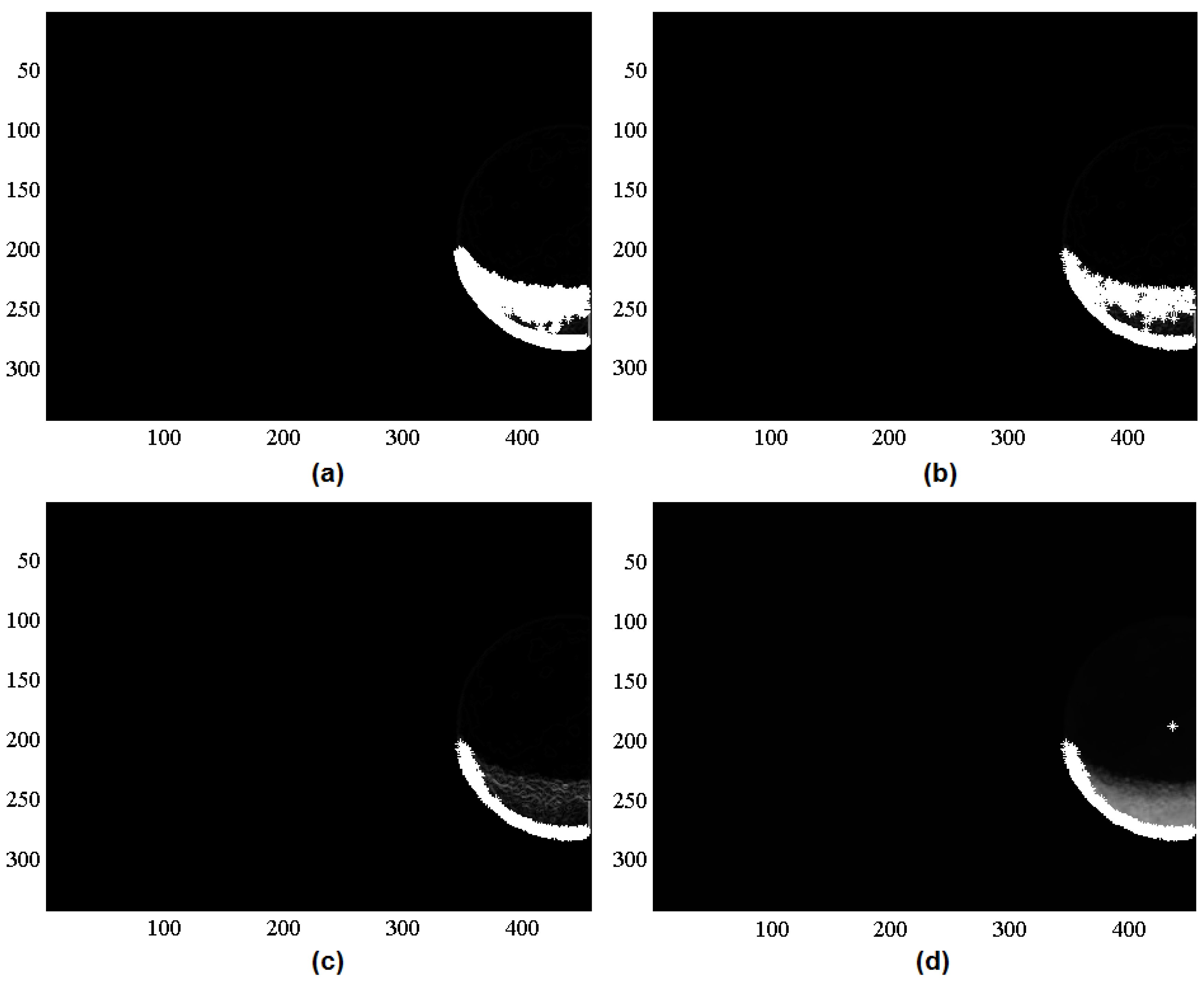
The original image of Example 1, shown in
Figure 9, was intentionally cropped from a real image (taken from Earth) to validate the capability of the software to face multiple cropped Moon images. Being cropped four times is also the maximum number of cropped segments possible. The four figures of
Figure 9 show the four main phases of the image processing. Once the image differentiation has been computed, the first 1490 points with the highest derivatives have been selected. This number differs from
, because the image is small, and the number of points selected is also a function of the total number of pixels (
is also the maximum number).
The box-based outliers elimination approach discarded 375 points, while RANSAC eliminated an additional five points. The resulting points are shown in the bottom right of
Figure 10 using white markers.
The bottom right of
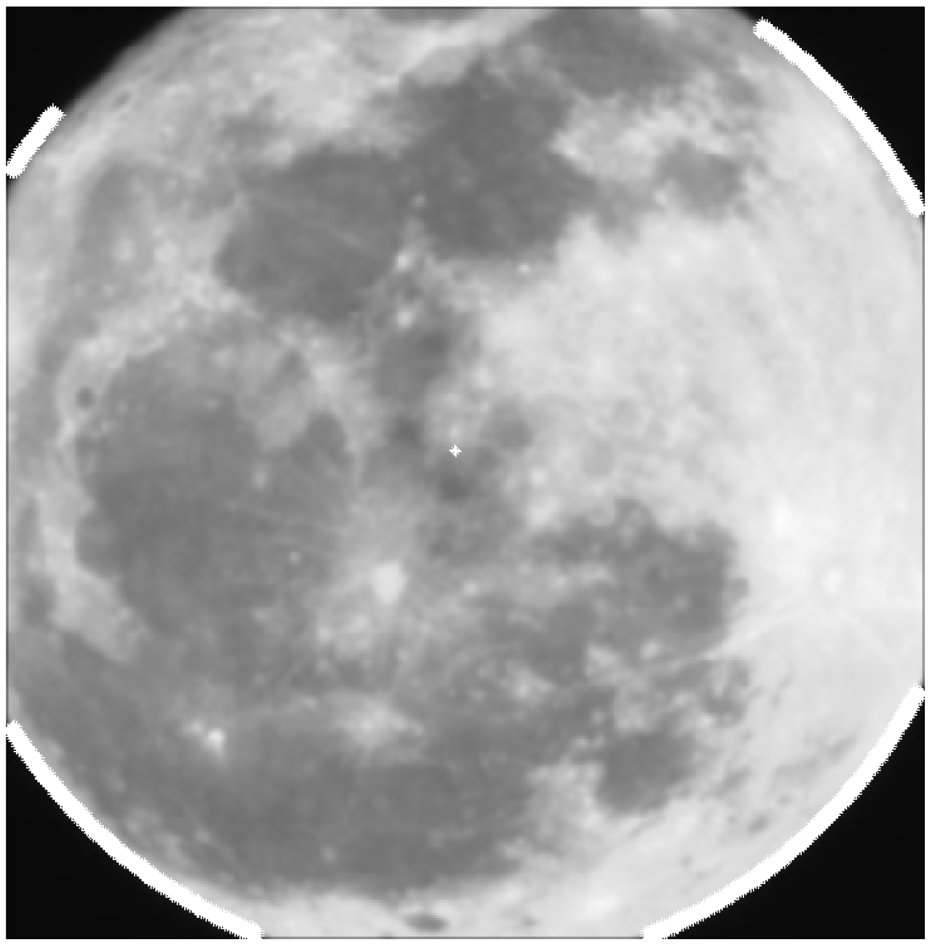
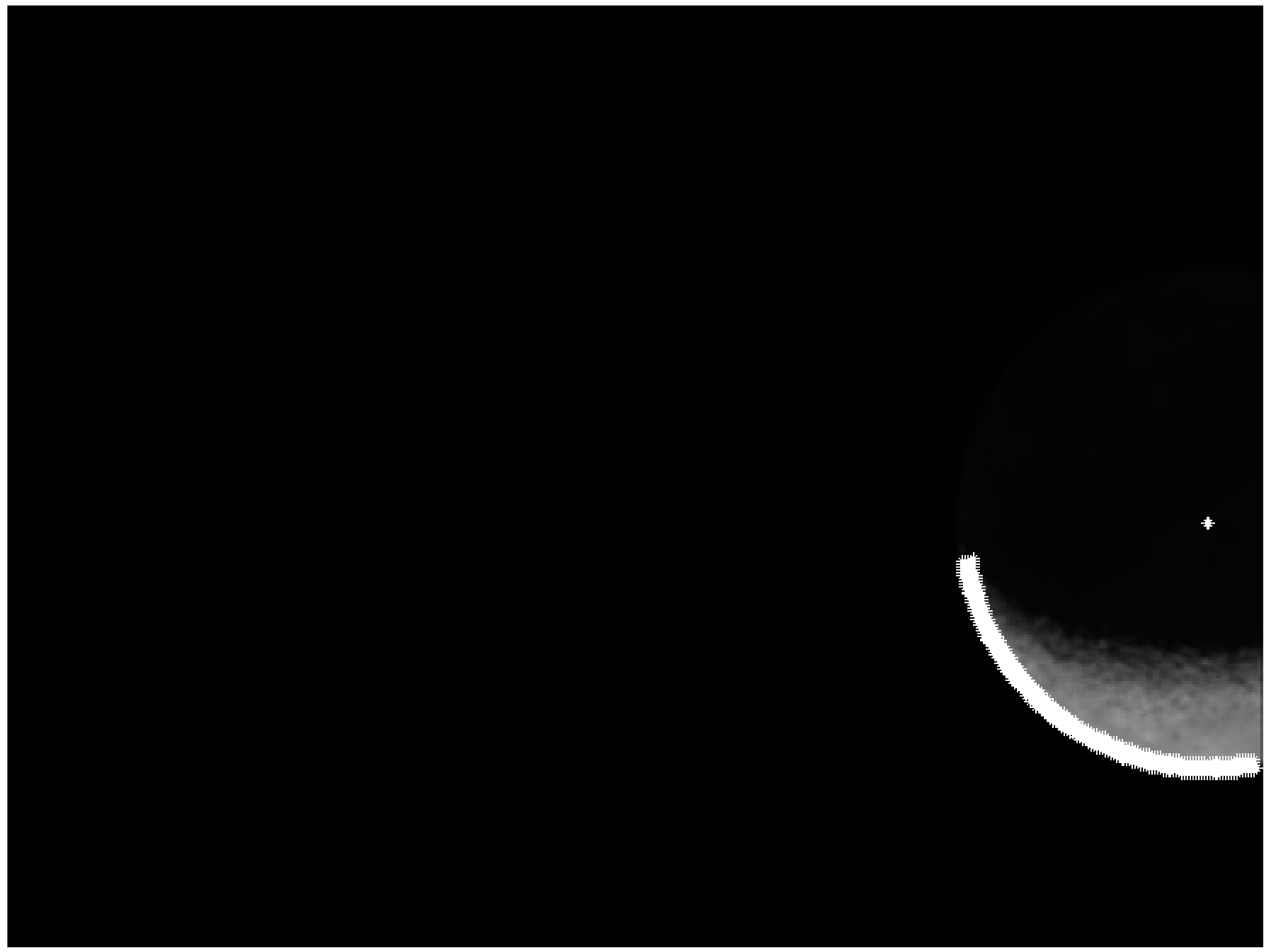
Figure 10 shows the results obtained by the Taubin fitting approach to estimate the circle parameters (Moon center and radius). The maximum distance from the estimated circle (worst residual) of the selected points was 2.9 pixels. The Taubin estimation gives a Moon center located at row 185.56 and column 187.34 and radius 218.03. Using this estimate, the set of points shown by white markers in
Figure 11 of the Moon edge have been selected. These points are then used by CSF-LS to perform the nonlinear least-square estimation of the Moon center and radius using the circular sigmoid function. The new estimate implies a variation of
,
and
pixels for row and column center coordinates and for radius, respectively.
Figure 9.
Example 1: Original image.
Figure 9.
Example 1: Original image.
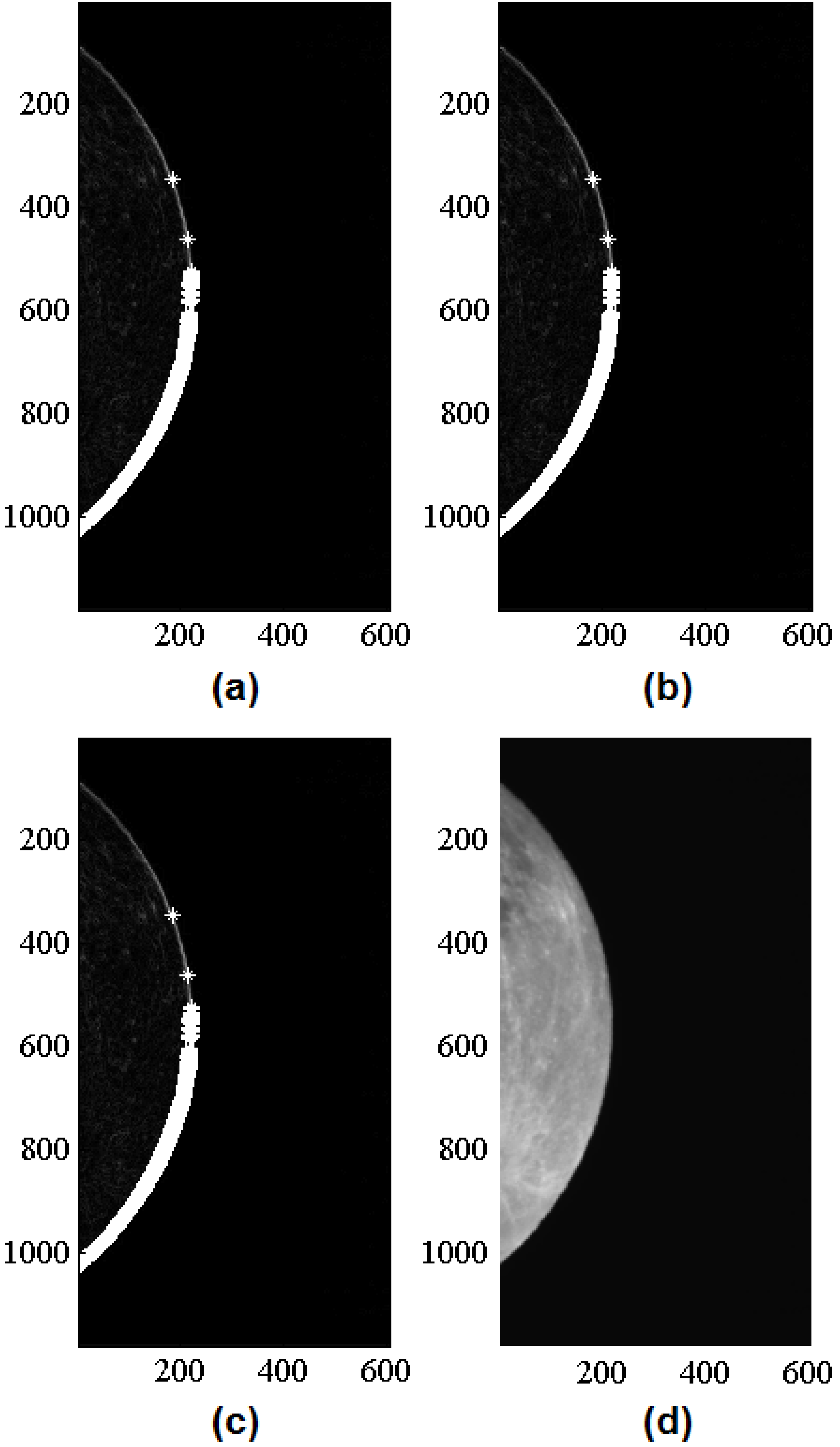
Figure 10.
Example 1: Image processing phases (data in pixel). (a) 1490 highest derivatives; (b) box approach removed 375 outliers; (c) RANSAC removed 5 outliers using 100 tests and ; (d) Body center inside image. Row center = 185.5991, Column center = 187.339, Radius = 218.0337 (worst residual = 2.9321).
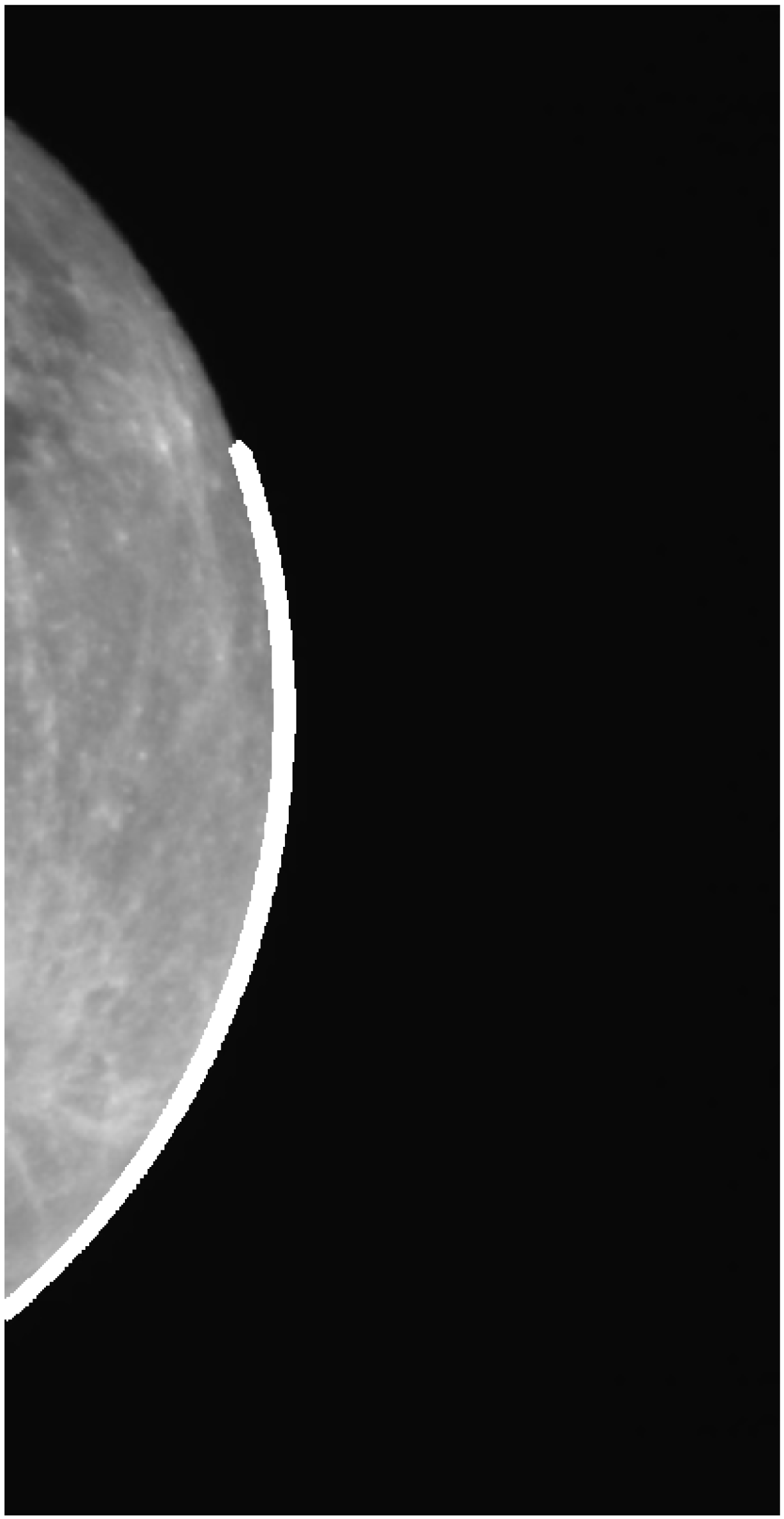
Figure 11.
Example 1: Circular Sigmoid Function (CSF)-LS final estimation. Center (white mark) inside the image. Row center: 186.169 pixel (). Column center: 187.8695 pixel (). Radius: 217.6452 pixel ().
Figure 11.
Example 1: Circular Sigmoid Function (CSF)-LS final estimation. Center (white mark) inside the image. Row center: 186.169 pixel (). Column center: 187.8695 pixel (). Radius: 217.6452 pixel ().
6.2. Example 2: Synthetic Image Cropped
In the second example, the test image is a synthetically-generated image. All of the relevant data and results are shown in
Figure 12,
Figure 13 and
Figure 14.
Figure 12.
Image convolution using a mask. (a): original image; (b) convoluted image.
Figure 12.
Image convolution using a mask. (a): original image; (b) convoluted image.
Figure 13.
Example 2: Image processing phases (data in pixel). (a) 1500 highest derivatives; (b) box approach removed 911 outliers; (c) RANSAC removed 229 outliers using 100 tests and ; (d) Body center inside image. Row center = 189.0829, Column center = 437.5094, Radius = 89.0182 (worst residual = 4.9575).
Figure 14.
Example 2: Circular Sigmoid Function (CSF)-LS final estimation (data in pixel). Center (white mark) inside the image. Row center: 189.2105 (). Column center: 437.1483 (). Radius: 89.0247 ().
Figure 14.
Example 2: Circular Sigmoid Function (CSF)-LS final estimation (data in pixel). Center (white mark) inside the image. Row center: 189.2105 (). Column center: 437.1483 (). Radius: 89.0247 ().
6.3. Example 3: Real Image with Center Far Outside the Imager
Figure 15.
Example 3: Original image.
Figure 15.
Example 3: Original image.
Figure 16.
Example 3: Image processing phases (data in pixel). (a) 1500 highest derivatives; (b) box approach removed 35 outliers; (c) RANSAC removed 0 outliers using 100 tests and ; (d) Body center outside image. Row center = 551.8926, Column center = −393.0706, Radius = 612.8029 (worst residual = 2.995).
Figure 17.
Example 3: CSF-LS final estimation (data in pixel). Center outside the image. Row center: 556.0114 (). Column center: −386.4042 (). Radius: 605.5698 ().
Figure 17.
Example 3: CSF-LS final estimation (data in pixel). Center outside the image. Row center: 556.0114 (). Column center: −386.4042 (). Radius: 605.5698 ().
7. Error Analysis
This section is dedicated to the error analysis associated with the following sources:
Estimated position error: This analysis quantifies how the error in the measured Moon radius (in pixel) affects the spacecraft-to-Moon distance computation (in km).
Estimated attitude error: This analysis quantifies how the error in the camera attitude knowledge affects the spacecraft-to-Moon direction (unit-vector).
Image processing errors: This Monte Carlo analysis shows the distribution of the Moon radius and center estimated by the image processing software when the image is perturbed by Gaussian noise. This is done in the three cases of crescent, gibbous and full Moon illumination.
7.1. Position and Attitude Uncertainty Propagation
This section investigates the sensitivity of the Moon estimated radius to the position estimation error. It also investigates the error in the Moon center direction because of the attitude estimation error.
The Moon radius (in pixel) is directly related to the spacecraft-to-Moon distance. The spacecraft-to-Moon vector is , where and r are the Moon and spacecraft position vectors in J2000, respectively. Vector is simply derived from time, while the spacecraft position vector, r, can be considered a random vector variable with mean and standard deviation , that is , where is a random unit-vector variable uniformly distributed in the unit-radius sphere. Neglecting the ephemeris errors, the uncertainty in the spacecraft vector position coincides with the uncertainty in the spacecraft-to-Moon distance, .
The Moon radius in pixels in the imager is provided by:
where
d is the pixel dimension (in the same unit of the focal length,
f),
= 1737.5 km is the Moon radius and
D is the spacecraft-to-Moon distance. This equation allows us to derive the uncertainty in the Moon radius in the imager:
The inverse of Equation (
37):
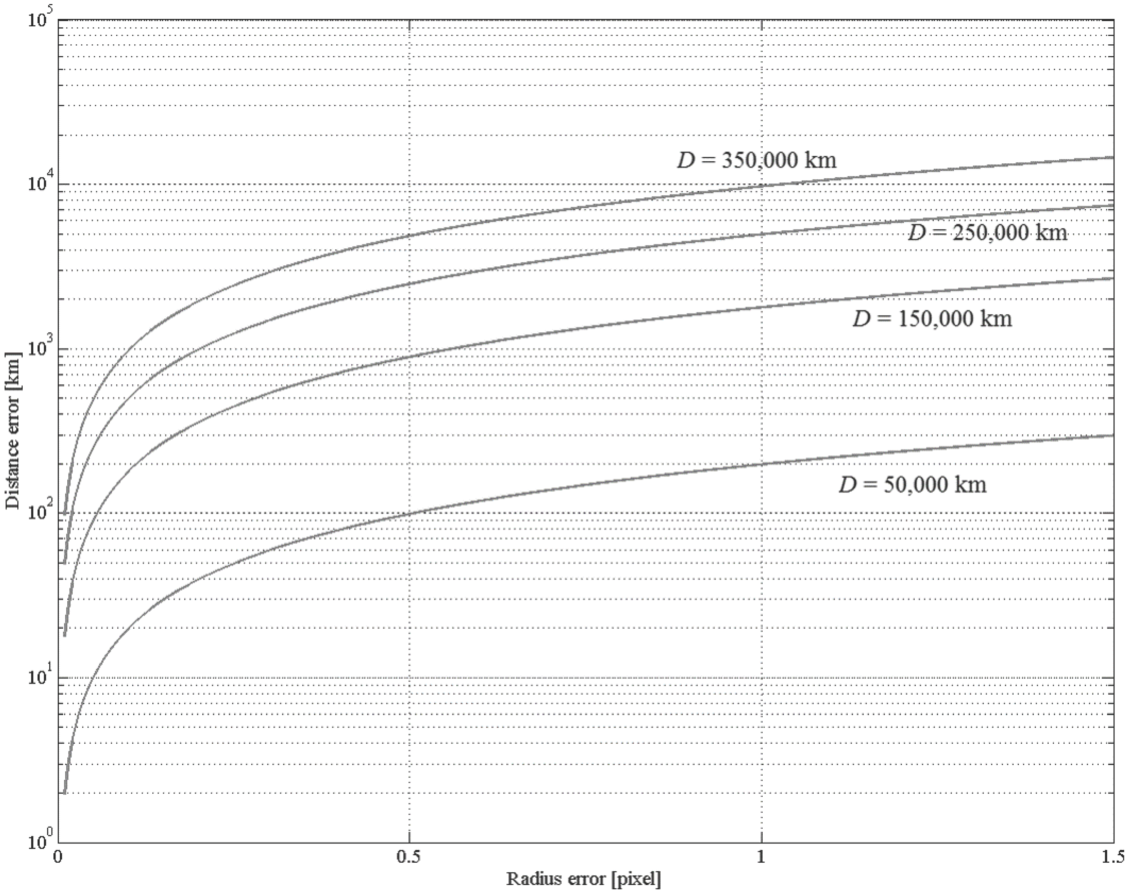
provides important information about the accuracy required by the radius estimation. This equation tells you how the radius estimate accuracy is affecting the spacecraft-to-Moon vector length and, consequently, how this estimate is affecting the estimation of the spacecraft position.
Equation (
38) has been plotted in
Figure 18 as a function of the Moon radius error and for four values of the Moon distance,
50,000 km,
150,000 km,
250,000 km and
35,000 km.
Figure 18.
Moon distance error vs. distance.
Figure 18.
Moon distance error vs. distance.
The Moon direction uncertainty (in pixels) is caused by the uncertainty in the attitude knowledge. Consider the attitude
with mean
and standard deviation
. The displacement with respect to the camera optical axis is
, where
ϑ is the angle between the estimated Moon center and the camera optical axis. Therefore, the radial uncertainty in the Moon center direction is provided by:
7.2. Image Processing Error
Image processing error quantification requires performing statistics using a substantial set of images with known true data. Since no such ideal database is currently available, the analysis of the resulting estimated parameters (Moon radius and centroid) dispersion is performed by adding Gaussian noise to the same image. The Moon illumination scenario plays here a key role, since when the Moon is fully illuminated, the number of data (pixels) used to perform the estimation will be twice as much as in the partial illumination case (under the same conditions: distance to the Moon and selected camera). For this reason, two scenarios have been considered:
Partially-illuminated Moon (results provided in
Figure 19);
Fully-illuminated Moon (results provided in
Figure 20).
Figure 19.
Image processing error results: partial illumination case.
Figure 19.
Image processing error results: partial illumination case.
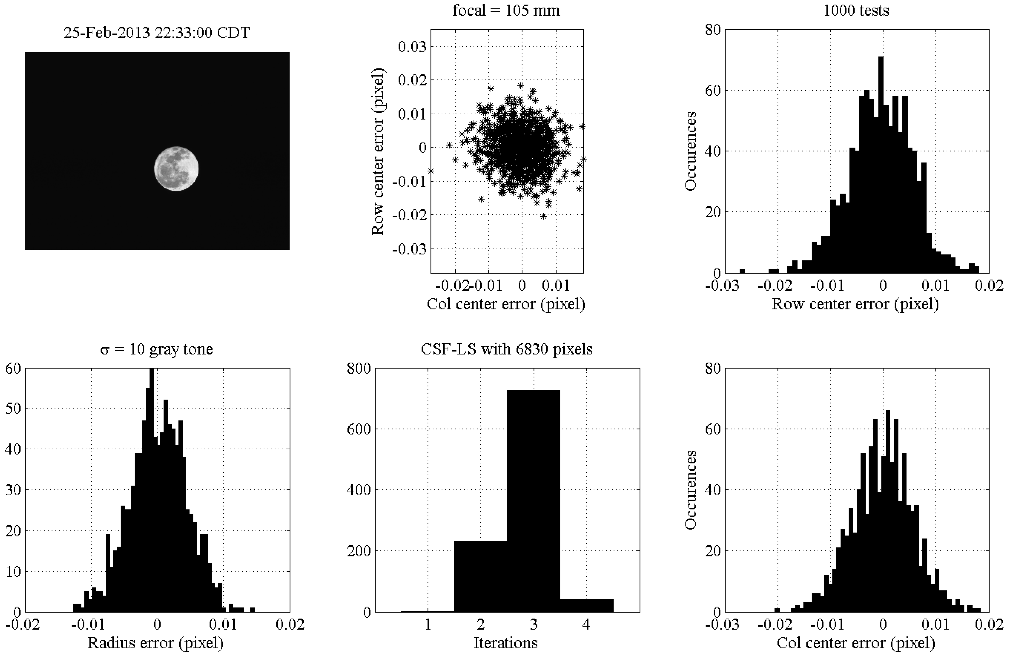
Figure 20.
Image processing error results: full illumination case.
Figure 20.
Image processing error results: full illumination case.
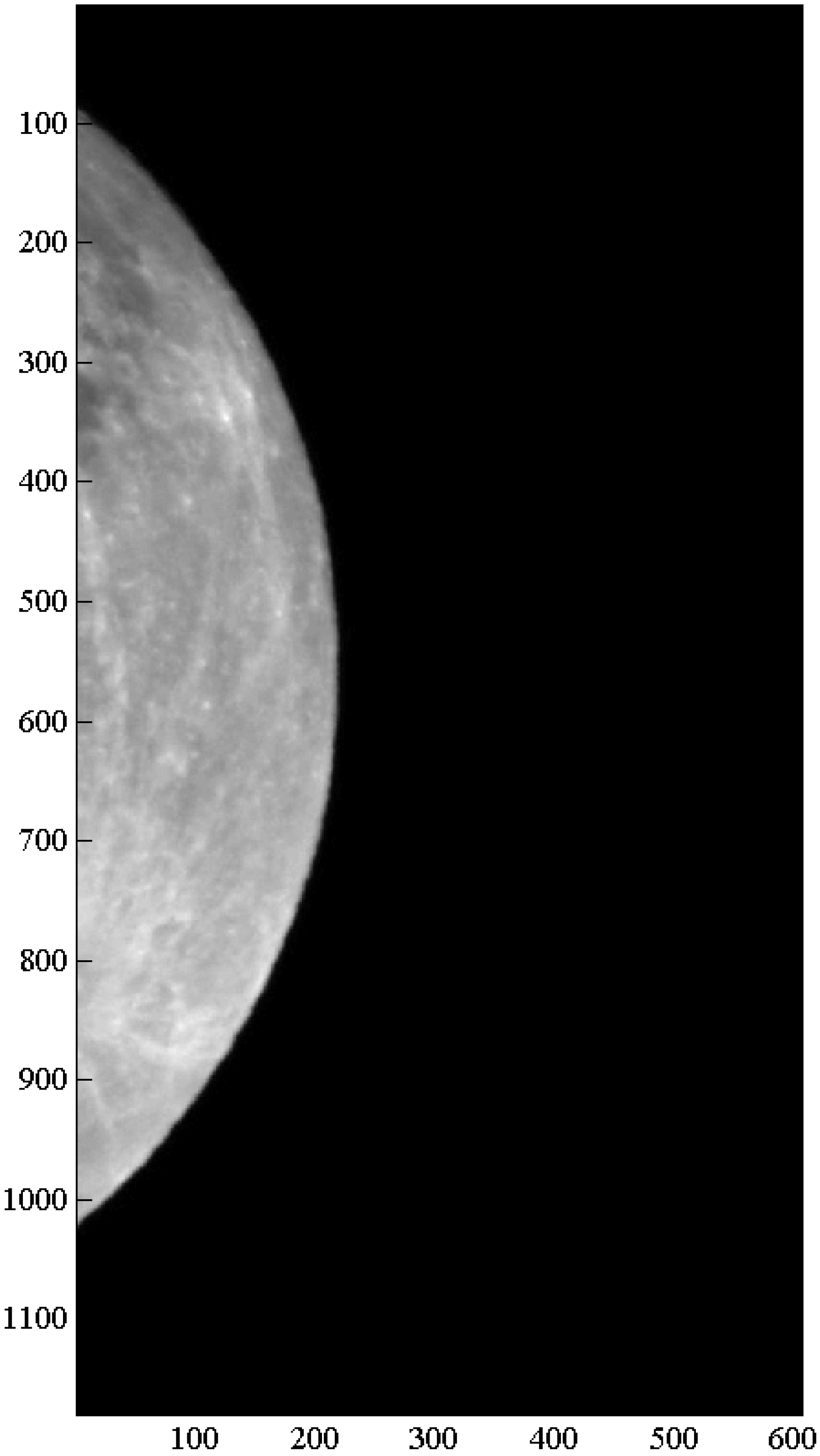
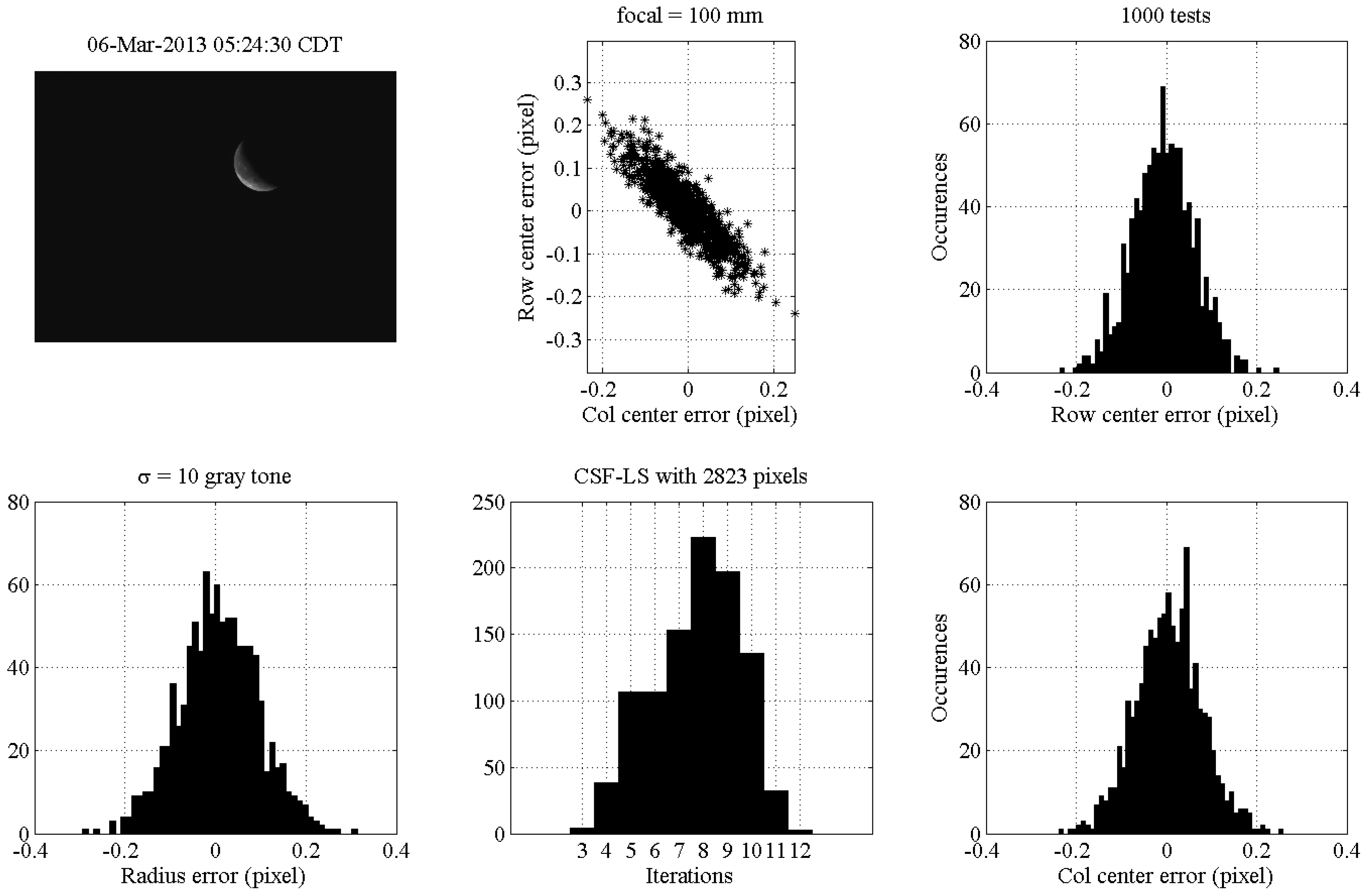
The results of the tests done using partially illuminated Moon are shown in
Figure 19. The image selected is real, and it was taken on 6 March 2013 at 05:24:30 using a focal length
mm. The statistics of the results obtained in 1000 tests by adding Gaussian noise with zero-mean value and standard deviation
gray tone are given. The code estimates the Moon radius and center (row and column) by least-squares using the circular sigmoid function (CSF-LS). The results show the three parameters estimated as unbiased and with a maximum error of the order of 0.2 pixels (with respect to the original picture). The histogram of the number of iterations required by the least-squares to converge shows an average of eight iterations. The central-upper plot in
Figure 19 shows the ellipsoid distribution of the Moon center error due to the fact that the estimation uses just data on one side of the Moon, on the illuminated part.
The results of the tests done using the fully illuminated Moon are shown in
Figure 20. Furthermore, in this case, the image is real and was taken in Houston on 25 February 2013 at 22:33:00 CDT using a focal length
mm. The statistics of the results obtained in 1000 tests by adding Gaussian noise with zero-mean value and standard deviation
gray tone are given. The code estimates the Moon radius and center (row and column) by least-squares using CSF-LS. The results show the three parameters estimated as unbiased and with a maximum error of the order of 0.01 pixels, one order magnitude being more accurate than what was obtained in the partial illuminated case. The histogram of the number of iterations required by the least-squares to converge shows an average of three iterations. The central-upper plot in
Figure 19 shows the unbiased Gaussian distribution of the Moon center error. These more accurate results are due to the fact that the estimation uses data all around the Moon edge.
8. Conclusions
This paper presents an image processing algorithm for visual-based navigation capable of estimating the observer to Moon vector. This information is then used for autonomous onboard trajectory determination in cislunar space. The proposed method first identifies the Moon edge pixels by numerical differentiation using Richardson extrapolation. This creates gradient images where most of the brightest pixels belong to the Moon edge. However, some of these pixels are generated on the Moon surface (outliers) due to the combination of illumination and Moon topology (craters). Two sequential filters are then adopted to remove these unwanted outliers. The first filter is provided by a box-based method that discriminates the edge pixels based on a local analysis of both the original and the gradient images, while the second filter is a standard RANSAC approach for circles. Once a subset of pixels belonging to the Moon edge has been identified, they are then used to perform the first (crude) estimation of the Moon centroid and radius. This is done in closed-form using Taubin’s method to perform least-squares best fitting estimation of a circle. This first estimate is then used to apply a subsequent accurate iterative nonlinear least-squares approach to estimate the Moon center and radius using circular sigmoid functions. Circular sigmoid functions accurately describe the actual gray tone smooth transition at the hard edge. In particular, this transition is described by a smoothing parameter, which is also estimated. Preliminary analysis of the algorithm’s performance is studied via processing both real and synthetic lunar images.
Acknowledgments
The authors greatly thank Dr. Chris D’Souza and Steven Lockhart of NASA-JSC for their direct and indirect contributions to this study.
Author Contributions
Daniele Mortari conceived of and developed the original theory. Francesco de Dilectis validated the idea by developing the software. Renato Zanetti supervised in detail the theory and validation and improved the use of English in the manuscript.
Conflicts of Interest
The authors declare no conflict of interest.
References
- Chorym, M.A.; Hoffman, D.P.; Major, C.S.; Spector, V.A. Autonomous navigation-where we are in 1984. In Guidance and Control; AIAA, Inc.: Keyston, CO, USA, 1984; pp. 27–37. [Google Scholar]
- Owen, W.; Duxbury, T.; Action, C.; Synnott, S.; Riedel, J.; Bhaskaran, S. A brief history of optical navigation at JPL. In Proceedings of the 31st AAS Rocky Mountain Guidance and Control Conference, Breckenridge, CO, USA, 1–6 February 2008.
- Synnott, S.; Donegan, A.; Riedel, J.; Stuve, J. Interplanetary optical navigation: Voyager uranus encounter. In Proceedings of the AIAA Astrodynamics Conference, Williamsburg, VA, USA, 18–20 August 1986.
- Riedel, J.E.; Owen, W.M., Jr.; Stuve, J.A.; Synnott, A.P.; Vaughan, R.A.M. Optical navigation during the voyager neptune encounter. In Proceedings of the AIAA/AAS Astrodynamics Conference, Portland, OR, 20–22 August 1990.
- Gillam, S.D.; Owen, W.M., Jr.; Vaughan, A.T.; Wang, T.-C.M.; Costello, J.D.; Jacobson, R.A.; Bluhm, D.; Pojman, J.L.; Ionasescu, R. Optical navigation for the Cassini/Huygens mission. In Proceedings of the AIAA/AAS Astrodynamics Specialist Conference, Mackinac Island, MI, USA, 19–23 August 2007.
- Li, S.; Lu, R.; Zhang, L.; Peng, Y. Image processing algorithms for deep-space autonomous optical navigation. J. Navig. 2013, 66, 605–623. [Google Scholar] [CrossRef]
- Christian, J.A.; Lightsey, E.G. Onboard image-processing algorithm for a spacecraft optical navigation sensor system. J. Spacecr. Rockets 2012, 49, 337–352. [Google Scholar]
- Christian, J.A. Optical navigation using planet’s centroid and apparent diameter in image. J. Guid. Control Dyn. 2015, 38, 192–204. [Google Scholar] [CrossRef]
- Mortari, D.; de Dilectis, F.; Zanetti, R. Position estimation using image derivative. In Proceedings of the AAS/AIAA Space Flight Mechanics Meeting Conference, Williamsburg, VA, USA, 12–15 January 2015.
- Taubin, G. Estimation of planar curves, surfaces and nonplanar space curves defined by implicit equations, with applications to edge and range image segmentation. IEEE Trans. PAMI 1991, 13, 1115–1138. [Google Scholar] [CrossRef]
- Fischler, M.A.; Bolles, R.C. Random sample consensus: A paradigm for model fitting with applications to image analysis and automated cartography. Comm. ACM 1981, 24, 381–395. [Google Scholar] [CrossRef]
- Mortari, D.; Samaan, M.A.; Bruccoleri, C.; Junkins, J.L. The pyramid star pattern recognition algorithm, ION. Navigation 2004, 51, 171–183. [Google Scholar] [CrossRef]
- Chernov, N. Circular and linear regression. Fitting circles and lines by least squares. In Monographs on Statistics and Applied Probability; CRC Press: Boca Raton, FL, USA, 2011; Volume 117. [Google Scholar]
© 2015 by the authors; licensee MDPI, Basel, Switzerland. This article is an open access article distributed under the terms and conditions of the Creative Commons Attribution license (http://creativecommons.org/licenses/by/4.0/).


