Prediction of Heat Transfer in a Jet Cooled Aircraft Engine Compressor Cone Based on Statistical Methods
Abstract
:1. Introduction
2. Experimental Procedure
2.1. Design Parameters
2.2. Design Parameter Space
3. Results and Discussion
3.1. Measurement Uncertainty
3.2. Sensitivity Study
3.3. Derived Correlation
3.4. Correlation Quality
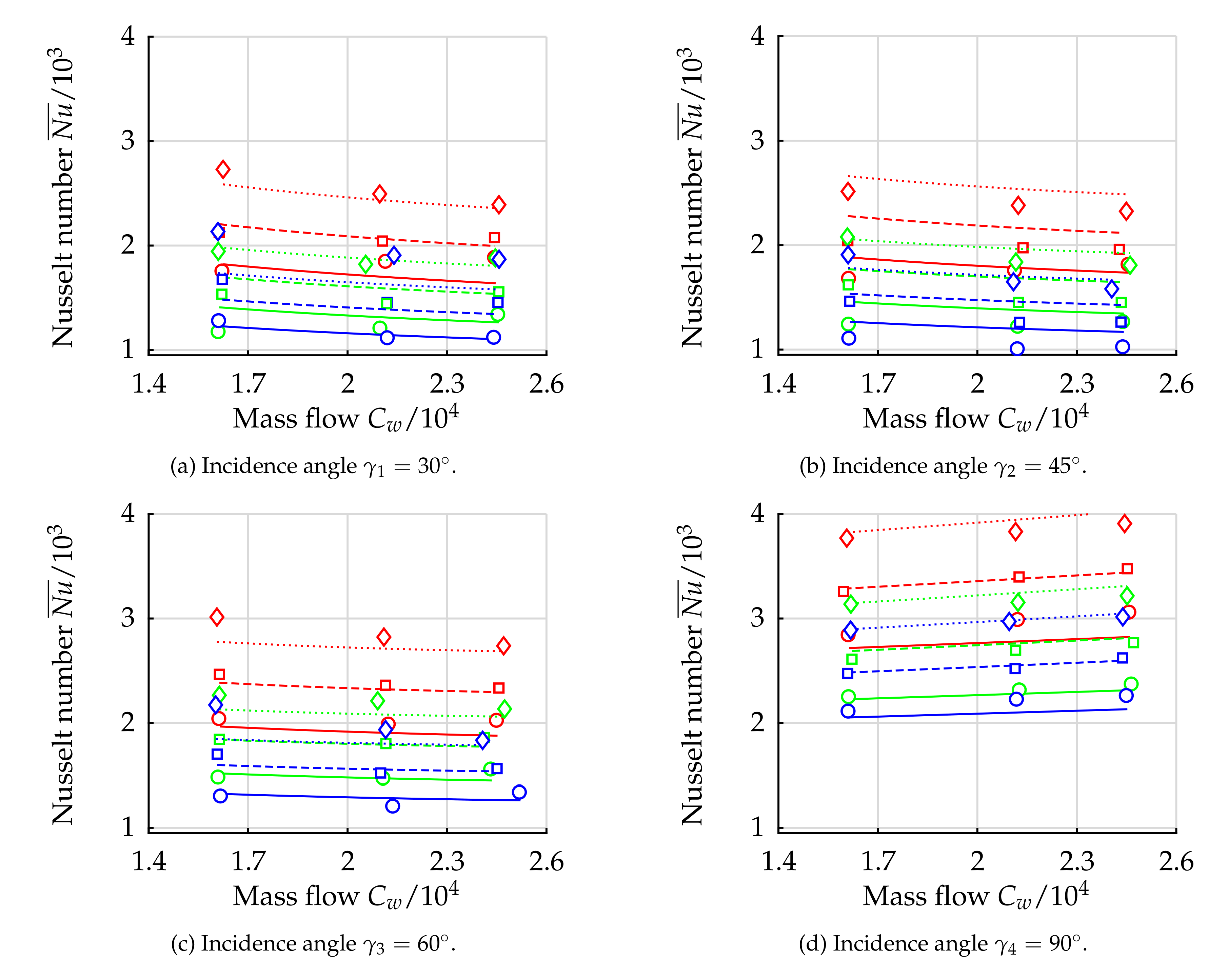
 ). In this case, the correlation shows a decreasing Nusselt number with increasing mass flow rate, while the experimental results indicate an increasing Nusselt number. The same trend can be observed for , and the relative spacing (
  ). For the case and (
  ) larger deviations of 20% can be found, whereas the qualitative dependency is predicted correctly. The comparison for the incidence angle according to Figure 10b shows a similar effect, but the correlation generally over predicts the Nusselt numbers and underestimates the influence of the mass flow rate for higher gap widths and . This trend can also be observed for the incidence angle depicted in Figure 10c, while the quantitative deviations between measured and predicted data is small. In case of the largest incidence angle both the qualitative and the quantitative agreement between predicted and measured data is excellent.
4. Summary and Conclusions
Author Contributions
Acknowledgments
Conflicts of Interest
Abbreviations
| Latin Symbols | |
| A | Area (m2) |
| d | Diameter (m) |
| C | Coefficient of a model (variable) |
| H | Structural thickness (m) |
| L | Characteristic length (m) |
| Heat flux (W) | |
| T | Temperature (K) |
| Volumetric flow (m3/s) | |
| W | Mechanical power (W) |
| cp | Specific heat (J/(kg K)) |
| e | Exponent of a model (–) |
| h | Heat transfer coefficient (W/m2/K) |
| k | Thermal conductivity (W/(m K)) |
| Mass flow (kg/s) | |
| n | Number of inlet holes (–) |
| p | Pressure (Pa) |
| Heat flux density (W/m2) | |
| r | Radial coordinate (m) |
| s | Gap width (m) |
| u | Radial velocity component u = ur (m/s) |
| z | Axial coordinate (m) |
| Greek Symbols | |
| Δ | Absolute uncertainty (variable) |
| γ | Incidence angle (rad) |
| μ | Dynamic viscosity (Pa s) |
| ν | Kinematic viscosity (m/s2) |
| ω | Angular velocity (rad/s) |
| ϕ | Angular coordinate (rad) |
| ρ | Density (kg/m3) |
| σ | Normal stress (N/m2) |
| θ | Cone angle (rad) |
| Non-dimensional Groups | |
| Bi | Biot number Bi = h · H/kS |
| Non-dimensional Groups | |
| Cw | Non-dim. mass flow Cw = /(μ · ro) = /(v · ro) |
| D | Non-dim. jet hole diameter D = d/(2 · ro) |
| Ec | Eckert number Ec = u2/(cp · ΔT) |
| G | Gap ratio G = s/ro |
| K1 | Core rotation factor at gap inlet K1 = (cos γ · ujet)/(ro · ϕ) |
| Nu | Nusselt number Nu = h · ro/kf |
| Global Nusselt number = ʃ Nu · ΔT dA/ʃ ΔT dA | |
| Pr | Prandtl number Pr = μ · cp/k |
| Re | Reynolds number Re = u · ro/v |
| X | Radius ratio X = ri/ro |
| R | Recovery factor R = Pr1/3 |
| Indices | |
| 1 | Gap inlet property |
| ad | Adiabatic |
| c | Cooled |
| f | Fluid |
| h | Heated |
| i | Inner |
| jet | Jet |
| o | Outer |
| ϕ | Circumferential |
| S | Solid |
| W | Wall |
| L | Leakage |
| Abbreviations | |
| RMSE | Root Mean Square Error |
Appendix A. Finite-Element Model
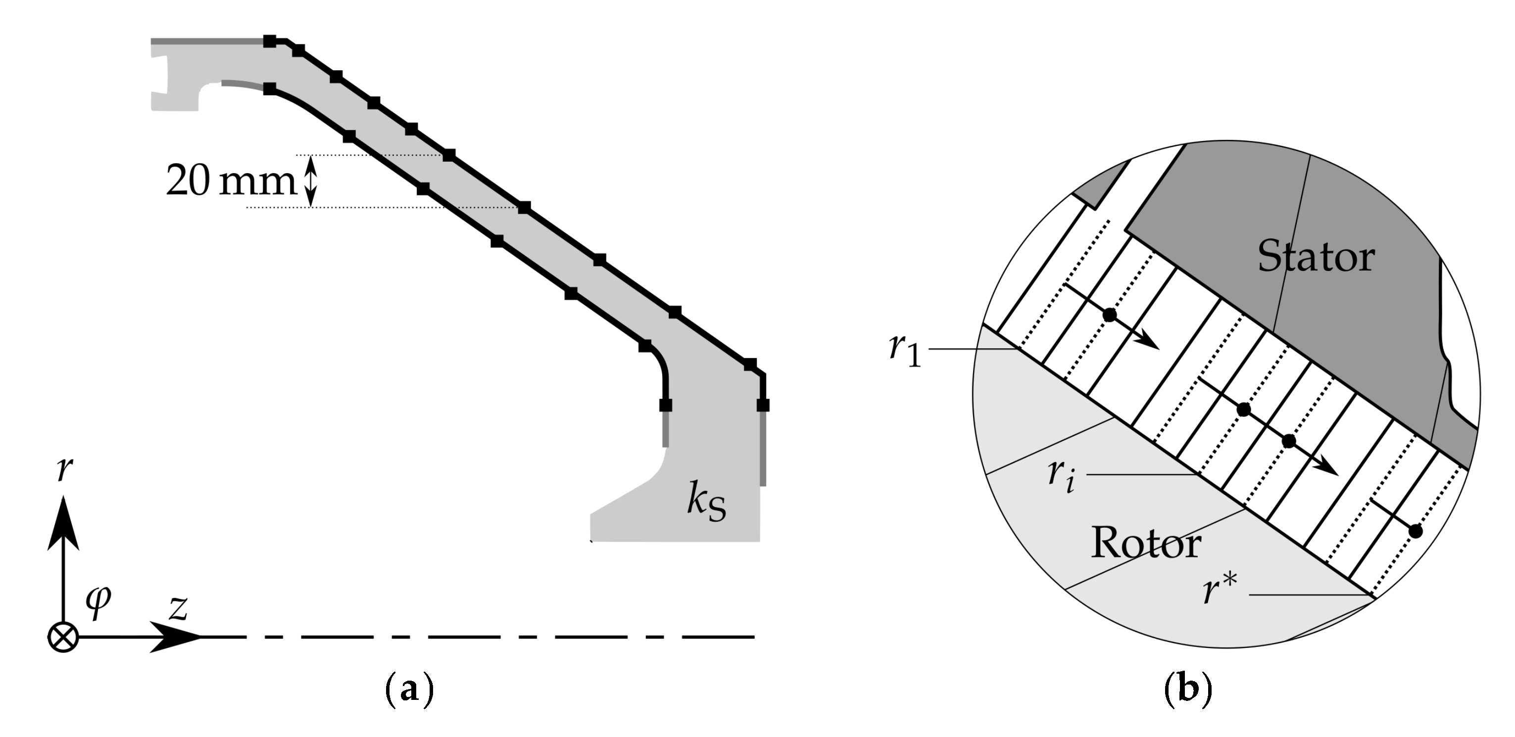
 ), extrapolated temperature (―). (b) Discretization of the rotor-stator gap to calculate the adiabatic wall temperature.
 ), extrapolated temperature (―). (b) Discretization of the rotor-stator gap to calculate the adiabatic wall temperature.
Appendix B. Adiabatic Wall Temperature
References
- Von der Bank, R.; Donnerhack, S.; Rae, A.; Cazalens, M.; Lundbladh, A.; Dietz, M. LEMCOTEC—Improving the Core-Engine Thermal Efficiency: Paper-Nr. GT2014-25040. In Proceedings of the ASME Turbo Expo 2014: Turbine Technical Conference and Exposition, Düsseldorf, Germany, 16–20 June 2014. [Google Scholar]
- Kervistin, R. Cooling System for a Gas Turbine Engine Compressor. U.S. Patent No. 5297386, 29 March 1994. [Google Scholar]
- Bleier, F.; Hufnagel, M.; Pychynski, T.; Eichler, C.; Bauer, H.J. Numerical Conjugate Heat Transfer Study of a Cooled Compressor Rear Cone: Paper-Nr. GT2014-26289. In Proceedings of the ASME Turbo Expo 2014: Turbine Technical Conference and Exposition, Düsseldorf, Germany, 16–20 June 2014. [Google Scholar]
- Bleier, F.; Höfler, C.; Pychynski, T.; Bauer, H.J. Design and Validation of a Test Rig for Heat Transfer Measurements on a Rotating Cone: Paper-Nr. ISABE-2015-20273. In Proceedings of the 22nd International Symposium on Air Breathing Engines, Phoenix, AZ, USA, 25–30 October 2015. [Google Scholar]
- Fénot, M.; Bertin, Y.; Dorignac, E.; Lalizel, G. A review of heat transfer between concentric rotating cylinders with or without axial flow. Int. J. Therm. Sci. 2011, 50, 1138–1155. [Google Scholar] [CrossRef]
- Harmand, S.; Pellé, J.; Poncet, S.; Shevchuk, I.V. Review of fluid flow and convective heat transfer within rotating disk cavities with impinging jet. Int. J. Therm. Sci. 2013, 67, 1–30. [Google Scholar] [CrossRef]
- Owen, J.M.; Rogers, R.H. Flow and Heat Transfer in Rotating-Disc Systems: Rotating Cavities; Research Studies Press: Taunton, UK; John Wiley & Sons: New York, NY, USA, 1995; Volume 2. [Google Scholar]
- Owen, J.M.; Rogers, R.H. Flow and Heat Transfer in rotating-Disc Systems: Rotor-Stator Systems; Research Studies Press: Taunton, UK; John Wiley & Sons: New York, NY, USA, 1989; Volume 1. [Google Scholar]
- Alexiou, A.; Hills, N.J.; Long, C.A. Heat Transfer in High-Pressure Compressor Gas Turbine Internal Air Systems: A Rotating Disc-Cone Cavity with Axial Throughflow. Exp. Heat Transf. 2000, 13, 299–328. [Google Scholar] [CrossRef]
- Wimmer, M.; Zierep, J. Transition from Taylor vortices to cross-flow instabilities. Acta Mech. 2000, 140, 17–30. [Google Scholar] [CrossRef]
- Long, C.A.; Turner, A.B.; Kais, G.; Tham, K.M.; Verdicchio, J.A. Measurement and CFD Prediction of the Flow within an HP Compressor Drive Cone. J. Turbomach. 2003, 125, 165–172. [Google Scholar] [CrossRef]
- Dorfman, L.A. Hydrodynamic Resistance and the Heat Loss of Rotating Solids; Oliver & Boyd: Edinburgh, Scotland, UK, 1963. [Google Scholar]
- Daily, J.W.; Nece, R.E. Chamber Dimension Effects on Induced Flow and Frictional Resistance of Enclosed Rotating Disks. J. Basic Eng. 1960, 82, 217–230. [Google Scholar] [CrossRef]
- Pellé, J.; Harmand, S. Heat transfer measurements in an opened rotor-stator system air-gap. Exp. Therm. Fluid Sci. 2007, 31, 165–180. [Google Scholar] [CrossRef]
- Mitchell, J.W.; Metzger, D.E. Heat Transfer From a Shrouded Rotating Disk to a Single Fluid Stream. J. Heat Transf. 1965, 87, 485. [Google Scholar] [CrossRef]
- Djaoui, M.; Dyment, A.; Debuchy, R. Heat transfer in a rotor-stator system with a radial inflow. Eur. J. Mecha.-B/Fluids 2001, 20, 371–398. [Google Scholar] [CrossRef]
- Tang, H.; Shardlow, T.; Michael Owen, J. Use of Fin Equation to Calculate Nusselt Numbers for Rotating Disks. J. Turbomach. 2015, 137, 121003. [Google Scholar] [CrossRef]
- Geis, T. Strömung und Reibungsinduzierte Leistungs- und Wirkungsgradverluste in Komplexen Rotor-Stator Zwischenräumen. Ph.D. Thesis, Department of Mechanical Engineering, University of Karlsruhe, Baden-Württemberg, Germany, 2002. [Google Scholar]
- Seber, G.A.F.; Wild, C.J. Nonlinear Regression; John Wiley & Sons, Inc.: Hoboken, NJ, USA, 1989. [Google Scholar]

 ) [4].
 ) [4].


 ), (
), (  ), (
), (  ); : (
  ), (
), (  ), (
), (  ); : (
  ), (
), (  ), (
), (  ).
).
 ), (
), (  ), (
), (  ); : (
  ), (
), (  ), (
), (  ); : (
  ), (
), (  ), (
), (  ).
).
| Parameter | Definition | Test Rig Conditions | Engine Conditions [8,9,18] |
|---|---|---|---|
| Circ. Reynolds number | < 5 · 106 | > 10 · 106 | |
| Non-dim. mass flow rate | 16 · 103 to 25 · 103 | 5 · 103 to 50 · 103 | |
| Relative gap width | 0.03 to 0.11 | >0.05 | |
| Incidence angle | to | to | |
| Jet diameter ratio | 6.82 · 10−3 | tbd | |
| Number of jets n | 48 | tbd | |
| Leakage mass flow rate | 8 · 103 | ||
| Diameter ratio | 0.45 | >0.4 | |
| Cone angle | 35° | 36° | |
| Initial swirl ratio | <1.4 | <1.5 | |
| Biot number | 0.2 to 5 | 0.1 to 5 | |
| Eckert number | <2 | <1 | |
| Prandtl number | 0.71 | 0.72 |
| Group | /106 | /104 | ||
|---|---|---|---|---|
| 1 | 3.08 | 1.61 | 0.03 | |
| 2 | 3.83 | 2.12 | 0.07 | |
| 3 | 4.57 | 2.45 | 0.11 | |
| 4 | – | – | – |
| − | ∘ | ∘ | ||
| − | ∘ | ∘ | + | |
| ∘ | ∘ | + | ||
| ∘ | + | + |
| in % | RMSE | in % | in % |
|---|---|---|---|
| 96.3 | 129 | −0.812 | 7.53 |
© 2018 by the authors. Licensee MDPI, Basel, Switzerland. This article is an open access article distributed under the terms and conditions of the Creative Commons Attribution (CC BY) license (http://creativecommons.org/licenses/by/4.0/).
Share and Cite
Bleier, F.; Schwitzke, C.; Bauer, H.-J. Prediction of Heat Transfer in a Jet Cooled Aircraft Engine Compressor Cone Based on Statistical Methods. Aerospace 2018, 5, 51. https://doi.org/10.3390/aerospace5020051
Bleier F, Schwitzke C, Bauer H-J. Prediction of Heat Transfer in a Jet Cooled Aircraft Engine Compressor Cone Based on Statistical Methods. Aerospace. 2018; 5(2):51. https://doi.org/10.3390/aerospace5020051
Chicago/Turabian StyleBleier, Fabian, Corina Schwitzke, and Hans-Jörg Bauer. 2018. "Prediction of Heat Transfer in a Jet Cooled Aircraft Engine Compressor Cone Based on Statistical Methods" Aerospace 5, no. 2: 51. https://doi.org/10.3390/aerospace5020051


