Application of the HPCMP CREATE^TM-AV Kestrel to an Integrated Propeller Prediction

Abstract

This article presents the results of a computational investigation of an integrated propeller test case using the HPCMP CREATE${}^{\mathrm{TM}}$-AV Kestrel simulation tools. There is a renewed interest in propeller-driven aircraft for unmanned aerial vehicles, electric aircraft, and flying taxies. Computational resources can significantly accelerate the generation of aerodynamic models for these vehicles and reduce the development cost if the prediction tools can accurately predict the aircraft/propeller aerodynamic interactions. Unfortunately, limited propeller experimental data are available to validate computational methods. An American Institute of Aeronautics and Astronautics (AIAA) workshop was therefore established to address this problem. The objective of this workshop was to generate an open access-powered wind tunnel test database for computational validation of propeller effects on the wing aerodynamics, specifically for wing-tip-mounted propellers. The propeller selected for the workshop has four blades and a diameter of 16.2 in. The wing has a root and tip chord of 11.6 and 8.6 in, respectively. Two different simulation approaches were used: one using a single grid including wind tunnel walls and the second using a subset grid overset to an adaptive Cartesian grid that fills the space between the near-body grid and wind tunnel walls. The predictions of both approaches have been compared with available experimental data from the Lockheed Martin low-speed wind tunnel to investigate the grid resolution required for accurate prediction of flowfield data. The results show a good agreement for all tested conditions. The measured and predicted data show that wing aerodynamic performance is improved by the spinning tip-mounted propeller.

1. Introduction

Recently, there has been a surge of interest in using propellers for small unmanned aerial vehicles, electric-powered vehicles, and urban air transportation concepts. In addition to the environmental benefits, Patterson et al. [1] mentioned up to a 90% reduction in the fuel consumption for an electric-powered aircraft compared with those using conventional internal combustion engines (ICE). Other advantages over ICE include increased efficiency, power independent of changes in altitude or flight speed, fewer parts, increased reliability, and reduced vibration as well as reduced noise [1]. However, a major drawback in the success of fully electric aircraft has been associated with the high weights of batteries. This issue should be overcome in the near future with advances in battery technologies to increase the battery specific energy levels (energy capacity per unit battery weight), but a short-term possible solution to this problem is improving the aerodynamic efficiency of an electric-powered aircraft.

According to Patterson et al. [1], if a cruise lift-to-drag ratio of greater than 20 can be achieved, electric aircraft concepts can become practical with current specific energy of batteries. These large cruise lift-to-drag ratios can be attained using an integrated distributed propulsion system. Note that in a tractor configuration, in which a propeller is placed in front of the aircraft, the propeller can drastically alter the aerodynamics of the lifting surfaces downstream of the propeller [2,3]. A careful integration of the propulsion system with airframe has the potential to increase the aerodynamic performance of the aircraft. Specifically, a distributed propulsion concept, in which there is a spanwise distribution of the propulsive thrust force, has received considerable attention recently.

An interesting example is the NASA’s X-57 distributed electric propulsion aircraft which has 12 high-lift propellers mounted on nacelle-pylons in the front of the wing leading edge [4]. Two more propellers are located at the wingtip which rotate in opposite directions of the wingtip vortices in order to reduce the induced drag. X-57 is part of the Scalable Convergent Electric Propulsion Technology and Operations Research subproject focused on the design of a distributed electric propulsion to reduce the cruise energy consumption (4.8 time less) of the piston-powered Tecnam P2006T aircraft [5]. The aircraft has been investigated and developed in four series of configurations with increased complexity named mods. Mod I is the Tecnam P2006T aircraft; Mod II used the Tecnam P2006T aircraft but converted it to a fully electric one. Mod III used a larger aspect ratio wing design and moved propellers to the wing tips. High-lift pylons are included in the Mod III but not the propeller blades. Mod IV is similar to Mod III but includes all high lift propellers. Recently, Duensing et al. [6] used experimental and computational efforts to generate the aerodynamic database of Mod III configurations; note that the effects of wing-tip propellers on the aerodynamic performance were not studied. The accurate measurement and prediction of propeller effects on the aerodynamic performance of a vehicle such as X-57 are very challenging tasks. Recent advances in the computational fluid dynamics (CFD) allow rapid and accurate prediction of the mutual interference between the propeller and the airframe.

If capturing the flow details is not required, one might use simulation models based on the actuator disk concept, in which the propeller is modeled as a disk of finite thickness [7,8]. The flow through disk is assumed to be inviscid. The load distribution of the disk is then used to simulate the jump in total pressure, total temperature, and velocity of the flow passing through the propeller. The load distribution can be known from experiments or estimated from the time-averaged blade loads over one period of revolution [9]. Several adopted actuator disk methods in CFD solvers allow defining the radial distribution of the load and the flow rotation based on a given angular velocity. Including an actuator disk in CFD is probably the most computationally cheap method of simulating a propeller. In addition, no boundary layer grid resolution is needed for the actuator disks due to invsicid flow assumption [10]. In a more advanced computational method, the propeller is modelled as a series of 2D airfoils, named elements and then to estimate the aerodynamic performance of each element moving from the blade hub to its tip, assuming that there is no flow interaction between these elements [11]. This method can approximate the thrust and torque acting on the blades from integrating calculated forces and moments on each element. Advanced computational methods to more accurately capture the propeller flow-field include fully resolved blade geometries; methods in which blades spin using Chimera or overset grids or methods in which the blades are fixed using and a sliding interface approach or others [3,12,13,14,15].

Unfortunately, there are limited experimental data available for validation of integrated propeller predictions. Some references include the work of Goble and Hooker [16] who used an actuator disk to model the spinning propellers of the P-3C Orion aircraft and then compared the predicted forces/moments and wing pressure distributions with available experimental data and a study by Hooker [17], who used pressure data on the pod/pylon of KC-130 tanker aircraft during two flight tests to validate the CFD predicted loads. Stokkermans et al. [18] examined the applicability of actuator-disk and actuator-line models to study the aerodynamics of a tip-mounted propeller configuration. The model predictions were compared with measurement data from a wind-tunnel experiment. Unfortunately, due to insufficient experimental data including flow details behind the propeller, the propeller prediction capability has not yet been validated for many integrated propeller configurations. The lack of experimental data for validating computational models of a distributed electric propulsion such as the X-57 Maxwell airplane has led to the establishment of the 1st American Institute of Aeronautics and Astronautics (AIAA) Workshop for Integrated Propeller Prediction (WIPP). However, it was decided to use a less complex configuration than the X-57 airplane for the first workshop, only considering a wing-tip-mounted propeller (Mod III without high-lift pylons). The objective of this workshop was to generate an open access-powered wind tunnel test database for computational validation of the effects of a wingtip-mounted propeller on the wing aerodynamics. This article specifically describes the use of the HPCMP CREATE${}^{\mathrm{TM}}$-AV Kestrel simulation tools to investigate the propeller wing aerodynamic interaction of this novel configuration. Fully resolved geometry blades are modeled in Kestrel using two different solves of KCFD and KCFD/SAMAIR. KCFD uses a second-order ccurate cell-centered finite volume discretization, however, SAMAir utilizes a fifth-order finite volume discretization on Cartesian meshes and allows adaptive mesh refinement. This work establishes a validated computational framework for wing/propeller interaction predictions.

2. CFD Solver

Kestrel is the fixed-wing product of the CREATE${}^{\mathrm{TM}}$-AV program funded by the DoD High Performance Computing Modernization Program (HPCMP). The objective of the CREATE${}^{\mathrm{TM}}$ program is to improve the Department of Defense acquisition time, cost, and performance using state-of-art computational tools for design and analysis of ships, aircraft and antenna. Kestrel is specifically developed for multidisciplinary fixed-wing aircraft simulations incorporating components for aerodynamics, jet propulsion integration, structural dynamics, kinematics, and kinetics [19]. The code has a Python-based infrastructure that integrates Python, C, C++, or Fortran written components [20]. Kestrel 10.4.1 is the latest release and used in this work. The code has been extensively tested and a variety of validation documents have been reported.

Kestrel CFD solvers include KCFD [21], COFFE [22], and KCFD/SAMAir [23]. The KCFD flow solver and the dual mesh KCFD/SAMAir are used in this study. KCFD uses a second-order accurate cell-centered finite volume discretization, however, SAMAir utilizes a fifth-order finite volume discretization on Cartesian meshes [24]. In more detail, the KCFD flow solver discretizes the Reynolds averaged Navier–Stokes (RANS) equations into a second-order cell-centered finite-volume form. The code then solves the unsteady, three-dimensional, compressible RANS equations on hybrid unstructured grids [25]. The KCFD flow solver uses the method of lines (MOL) to separate temporal and spatial integration schemes from each other [21]. The spatial residual is computed via a Godunov type scheme [26]. Second-order spatial accuracy is obtained through a least squares reconstruction. The numerical fluxes at each element face are computed using various exact and approximate Riemann schemes with a default method based on the HLLE++ scheme [27]. In addition, the code uses a subiterative, point-implicit method (a typical Gauss–Seidel technique) to improve the temporal accuracy. Some of the turbulence models available within Kestrel include Spalart–Allmaras (SA) [28], Spalart–Allmaras with rotational/curvature correction (SARC) [29], Menter’s SST [30], and delayed detached Eddy simulation (DDES) with SARC [31].

Kestrel can include fully resolved blades, however, the propeller grid should be individually generated. The propeller flow-field can be simulated using a sliding interface approach for a non-spinning propeller or using an overset grid approach for spinning propellers. In addition, the code allows a thin actuator disk approach with uniform and non-uniform load distributions. A non-uniform case requires a given radial position for maximum thrust force. The loading profile is assumed to be linear with a zero thrust at the inner blade radius and then increases until the radial position of maximum thrust, then decreases to zero at the rotor tip. The blade element momentum modeling has been recently included in Kestrel version 11.0.

The Kestrel’s off-body Cartesian flow solver, SAMAir, can capture higher fidelity flow features (e.g., wakes) away from the primary body. SAMAir uses an overset grid approach in which the “near-body” grid is overset to the “off-body” Cartesian grid. The near-body grid can be generated from an existing grid using the subset mesh manipulation method. This subset grid should include the prism layers on the no-slip surfaces, i.e., the off-body grid should not be used to capture the boundary layer at these surfaces. The off-body grid, on the other hand, fills the computational space between the near-body and far-field boundary. An overset fringe is used where these two grids overlap. Using adaptive mesh refinement (AMR), the Cartesian solver can automatically refine the mesh around the regions of interest, and therefore, increase the solution accuracy where it is needed. The code only needs the extent of far-field boundary and the maximum number of grid refinement levels.

3. Test Case

The configuration used in the 1st AIAA Workshop for Integrated Propeller Prediction consists of a wing and a wingtip-mounted propeller resembling a 40.5% model scale of the X-57 airplane. The geometry details are given in Figure 1. The wing has a leading-edge sweep angle of 1.9 deg, a tip chord of 8.6 in, a root chord of 11.6 in, an aspect ratio of 6.7, and a mean aerodynamic chord of 10.15 in. The 10%-scale C-130 4-blade propeller with a diameter of 16.2 inches has been used and mounted on a pylon at the wing tip. The pylon length and maximum diameter measure 24.15 and 4.75 inches, respectively. The propeller blade angle was set at 37.5 deg to provide representative thrust and advance ratio values at tested airspeeds. Test cases include an isolated wing with spinner geometry and the wing with propeller blades. The isolated wing was used to establish a baseline to investigate the propeller effects. All models contain a splitter plate fairing at the wing root which was 17.25 inches long and 6.0 inches wide. This splitter plate is attached to a fused deposition modeling fairing, which allows the splitter plate to be 6.4 inches from the tunnel floor. Hooker et al. [32] provide more details of tested geometries.

Six spanwise positions were selected for pressure tap measurements, including two behind the propeller disk. The configuration was mounted vertically on the wind tunnel floor and a boundary layer diverter was used to eliminate the effects of boundary layer formed at the tunnel lower wall on the wing aerodynamic performance. Notice that in Figure 1a, blue-colored surfaces are only used to account for forces/moments imposed on the wing surface. The red-colored surfaces are used to measure propeller thrust and torque. In denoting forces and moments, the term “TC” shows thrust corrected, i.e., thrust has been removed from the total forces/moments measured at the load balance. The moment reference point is located at (2.99, 0.28, 6.35) inches and is highlighted in Figure 1b.

4. Experimental Apparatus

Hooker et al. [32] detail the conducted experiments. In summary, the WIPP configuration was tested in the lockheed Martin low speed wind tunnel, which is a conventional single return, atmospheric pressure, closed test section facility. Test section size measures as 16.25 × 23.25 × 43 ft with a 9000 HP (6700 kw) motor. The tunnel top speed is 90 m/s. The WIPP model was positioned vertically in this tunnel, Figure 2a, over a turnable plate. Experiments include isolated wing (no propeller blades), prop-off, and prop-on tests at different Mach numbers and angles of attack. The measurements include wing integrated forces and moments, pressure tap data at six spanwise locations, and a wake survey taken at several locations aft of the propeller. The pressure tap positions can be seen in Figure 2a where the leading edge paint is colored white at tap positions. The vertical and horizontal wake survey measurements can be seen in Figure 2a,b. The rake was moved to 5 locations behind the propeller and flow parameters, which were measured at every 0.2 in along wake strip. Power-on conditions were tested at thrust coefficients of 0.04, 0.2, and 0.4, where the thrust coefficient is defined as:

$$CT=\frac{T}{q_{\infty }{S}_{ref}}$$

(1)

where T is the propeller thrust, $q_{\infty }=0.5\rho V^2$ is the free-stream dynamic pressure, and $S_{ref}$ is the wing planform area of 675.6 in${}^2$.

Tunnel conditions were set to Mach numbers of 0.08 and 0.11 at sea-level conditions. The angles of attack tested include [0, 5, 7, 9, 11, 13, 15, 17] deg.

Table 1. Simulation test matrix.

Solver	Isolated Wing	Prop-Off	Prop-On	Mach	AoA [Deg]
KCFD	Yes	Yes	CT = [0.04, 0.2, 0.4]	0.08	[0, 5, 7, 9, 11, 13, 15, 17]
KCFD/SAMAIR	No	Yes	CT = [0.04, 0.2, 0.4]	0.08	[0, 5, 7, 9, 11, 13, 15, 17]

summarizes the simulation cases of this study.

5. Computational Grids

Two different computational grids have been tested: grids with farfield boundaries that match the wind tunnel walls and subset grids that overset to a background Cartesian grid. These grids have been used to investigate the grid resolution required for accurate prediction of flowfield data. Computational grids including the wind tunnel walls are referred to as “RANS” grids in this article. Wing and propeller grids were generated individually; the propeller grid was then overset to the wing grid. Figure 3 shows the wing geometry relative to the walls in the RANS grids. The overset boundary is shown in this figure as well. In this work, all wing and propeller surfaces were modelled as no-slip walls. The tunnel floor was modeled as a slip wall to eliminate the need for generating prism layers to capture the boundary layer. All other tunnel walls were modeled as far-field.

In more detail, computational grids were generated in Pointwise version 18.0. The surface grid cells are mostly structured quadrilaterally, but anywhere that these cell types are not possible to make, triangular surface cells are used. The interface between structured and unstructured mesh uses the surface T-rex technique, which ensures high quality transition between the structured and unstructured surface meshes. The main motivation for using the quadrilateral mesh is to have very good grid resolution on the blade leading and trailing edges and at the blade tips. A part of the hub is covered with patches of structured meshes as well. The volume mesh is fully unstructured with 50 prism layer on the propeller surface. The growth ratio of the prism layer is 1.25 and the growth is terminated when the transition between the prism layer and the tetrahedral mesh is smooth.

The wing grid including the tunnel volume has around 83 million cells. The propeller grid has an overset boundary with a diameter of about 1.5 times of blade diameter. This grid has around 19 million cells. Some grid images are given in Figure 4.

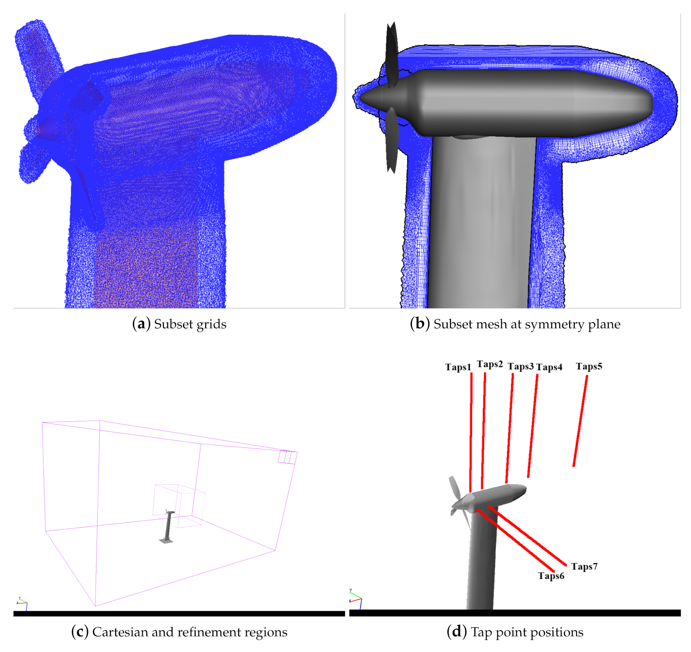
For Kestrel simulations, subset grids of the wing and propeller were generated. The subset grids are clipped at a normalized distance of 4 inches from the walls. The subset grid should include the prism layers to capture the boundary layer formed over the no-slip walls. The subset grids are shown in Figure 5a,b. The wing and propeller subset grids contain about 23.2 and 18.3 million cells, respectively. These subset grids are overset to a background Cartesian grid with 200-inches distance in front, back, and above the model. The sides have a distance of 138 inches. The lower surface is at the wind tunnel floor. All sides were assumed to be a farfield, but the bottom side was assumed to be a slip wall. A refinement region was defined around and behind the propeller. The Cartesian grid extent and the refinement region can be seen in Figure 5c. Seven tap locations were defined to match the wake survey measurements in the wind tunnel. These tap positions are shown in Figure 5d. Five positions are placed vertically relative to the propeller. Two are positioned in horizontal locations. Tap positions 1 to 5 have offsets of 2.65, 6.150, 14.150, 22.150, 42.150 inches relative to the propeller disk. Horizontal tap positions 6 and 7 have 2.65 and 6.150 offset distance relative to the propeller disk as well. Velocity components, density, static and stagnation pressure values were measured at these positions. In the simulations, these flow parameters were written at each time step for the final 1000 time steps. Time-averaged data were then calculated from these values.

6. Results and Discussions

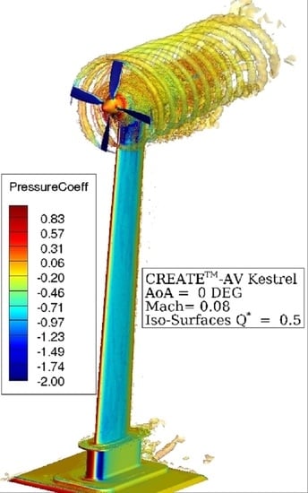
Only the Mach 0.08 case was considered in this study. Kestrel-KCFD and Kestrel-SAMAir flow solvers with the DDES-SARC turbulence model were used. First results correspond to the validation of propeller thrust and torque with available measured data at thrust coefficients of 0.04, 0.2, and 0.4. For validation purposes, the wing and propeller cases were run with different propeller spin rates ranging from 2000 to 7000 rpm. The RANS grid with five Newton sub-iterations was used. A time step of 0.0001 s and a temporal damping coefficient of 0.01 were used in all these simulations. The simulations were run for 5500 time steps with the propeller beginning to spin at $t=0.05$ s. For each case, the thrust and torque applied to the propeller blades (red surfaces in Figure 1a) were calculated in Kestrel. These data were compared with experimental data at three spin rates and are shown in Figure 6. Good agreement was found between CFD and experimental data. Note that there is no thrust force for spin rates below 2800 rpm. The force generated by the propeller at these low spin rates is an additional drag force on the whole configuration.

The following results are focused on the isolated wing (no propeller blades). Kestrel was run in an unsteady mode (second-order accuracy in time) with a time step of 0.001 s and three Newton sub-iterations. Only RANS grids were used. Simulations were run for 5500 iterations, including 500 start-up iterations. The start-up iterations are usually helpful to have a robust startup capability before a motion begins, e.g., propeller spin or control surface deflection. Note that physical time will be held fixed at zero during these iterations. Temporal damping coefficient was set to 0.01 as well. The solutions for the final two seconds were time averaged. Simulations were run for angles of attack of [0, 5, 7, 9, 11, 15, 17] degrees. Figure 7 compares the predicted drag polar and pitch moment values with measured data for an isolated wing. Figure 7 shows that CFD data agree well with experimental data up to nine degrees angle of attack. At higher angles, CFD predicts larger drag values and a steeper pitch moment curve slope. In addition, CFD data predict slightly larger lift values for angles between 7 and 9 degrees.

Figure 8 compares the flow solutions and wing surface pressure data at six spanwise locations of an isolated wing with experimental data at angles of attack of 0, 5, and 15 degrees. The pressure tap locations are shown in Figure 8 as well. Good agreement can be seen between predicted and measured pressure data at most locations. At AoA = 15${}^{\circ }$ and the tap position near the tip (BL 63.469 inches), discrepancies can be seen between CFD and experimental data in the leading edge and mid section of the upper wing surface (curve section with negative pressure coefficients). At this section, CFD predicts a separated flow region starting at 0.1 chord with flow re-attachment at 0.4 chord. Experiments show no flow separation.

Next, the wing with a powered-off propeller is simulated using RANS and SAMAir grids. The powered-off propeller is denoted as $CT=0$. These simulations were run for 7500 time steps. The mesh refinement begins at iteration 3600 with refinement at every 250 iterations based on the scaled Q-Criterion. Time step is 0.001 s. Off-body temporal damping coefficient was set to 0.025. Three Newton sub-iterations were used.

Figure 9 compares the isolated wing predictions with wing/propeller predictions using RANS and SAMAir grids. Note that the blade forces and moments were included in the shown integrated forces and moments. The non-spinning propeller will increase the drag force compared with the isolated wing. At small angles of attack, the lift is slightly smaller than for the isolated wing as well. Both RANS and SAMAir predictions agree well with each other up to 9 degrees angle of attack. At larger angles, the SAMAir data have drag coefficients similar to the isolated wing (decreasing lift at these angles), but the RANS grid shows increasing lift at large angles of attack.

In more detail, Figure 10, Figure 11 and Figure 12 compare the wing surface pressure data of an isolated wing with a wing/propeller with $CT=0$ using RANS and SAMAir grids. At small angles of attack, the propeller has no effect on the pressure data at Tap positions far from the propeller disk (Taps 34.38, 44.38). At other tap positions, especially those behind the propeller, the non-spinning propeller impacted the wing’s pressure distribution, in particular the leading-edge section. For angles of attack of zero and five degrees, RANS and SAMAir grids show very similar pressure plots. At 15 degrees angle of attack, SAMAir predicts less pressure data at the upper surface than RANS grid for Tap positions BL 34.386 and 44.386. Other tap positions have better agreements between SAMAir and RANS grids.

Figure 13 compares the flow solution of wing and powered-off propeller simulations using RANS and SAMAir grids at angles of attack of 0, 5, and 15 degrees. Contours of pressure coefficient and iso-surfaces of zero x-velocity are shown. Figure 13 shows that both RANS and SAMAir grids have similar pressure coefficient data at angles of 0 and 5 degrees. At 15 degrees angle of attack, there are different pressure values at the wing’s upper surface at the wing’s root and mid-sections. The SAMAir simulations show smaller pressure regions near the trailing edge. SAMAir simulations also show a larger separated flow region at the wing’s trailing edge than the RANS grid. Finally, for angles of 0 and 5 degrees, both grids show similar separated flow regions, however, SAMAir shows more details of the eddies formed in the separated region than RANS grid.

In the final simulations, the propeller rotates at different rates to match thrust coefficients of 0.04, 0.2, and 0.4. Simulations are again run with RANS and SAMAir grids. Five Newton sub-iteraions with a time step of 0.00005 s were used. Refinement frequency was set to every five time step. Figure 14 compares the drag polar plots of the isolated wing with wing/propeller at three different thrust settings. Note that in Figure 14a, the thrust force was included in the shown forces but it has been removed in the plots of Figure 14b. Figure 14a shows that CFD data predicted with RANS and SAMAir grids match well with each other and experimental data at all thrust settings, though for the highest $CT$ value the discrepancy between predictions and experimental data was higher than for the other $CT$ values. Figure 14b shows that a wingtip-mounted propeller will improve the wing aerodynamic performance as less drag and larger lift values are predicted compared with a no-propeller case.

Figure 15 shows the effects of the propeller at different thrust coefficients on the wing pressure distribution. No pressure differences can be seen between the isolated wing and integrated wing/propeller at pressure taps located far from the propeller disk. Closer to the propeller disk, the pressure differences between upper and lower surfaces become larger with increasing thrust coefficient. This is due to increased dynamic pressure behind the propeller and the changes in local angle of attack due to propeller rotation. This means that the wing will experience higher local lift at these locations. In more detail, Figure 16 shows the propeller slipstream for thrust coefficients of 0.04, 0.2 and 0.4. The slipstream becomes stronger with increasing thrust coefficient, as shown in this figure. Notice the highly reduced pressure regions formed over the wing upper surface due to the spinning propeller. The pressure becomes smaller as the propeller spins at higher rates.

Finally, Figure 17 and Figure 18 compare the x-velocity to free-stream ratio at wake tap positions 1, 3, 4, and 5, with experimental data for thrust coefficients of 0.2 and 0.4. RANS and SAMAir grids agree well in most locations. The figures show how the velocity (dynamic pressure) behind the propeller disk will increase with thrust coefficient. The velocity ratio becomes larger with increasing spin rate. The profiles (CFD and experiment) remain similar for all shown tap positions. The propeller effects of increased velocity can be seen even at a distance of 42.15 inches behind the propeller disk (or 2.6D). Again, CFD data match well with experiments except for thrust coefficient of 0.4, where CFD predicts a larger velocity increase at tap positions 3 and 4. CFD data show a reduced velocity region (velocity ratio less than 1) at tap 1 position just near the propeller tip. These reduced velocity regions are not seen in experimental data.

7. Conclusions

This article applies the Kestrel simulation tools to the test cases of the 1st AIAA Workshop for Integrated Propeller Prediction (WIPP). Two computational approaches were used: Kestrel-KCFD using a grid that models wind tunnel walls and Kestrel-SAMAir that uses subset grids overset to a background Cartesian grid. Simulations include an isolated wing, wing with a powered-off propeller, and wing-propeller at different thrust coefficients. The predictions were compared with the available experimental data. The results show good agreement with experiments in most cases, specifically at low angles of attack. The effects of powered-on and powered-off propellers on the wing aerodynamic performance were discussed. The spinning propeller (tested in this work) will generate reduced pressure regions on the wing upper surface behind the propeller disk. This is due to the increased local angle of attack and increased dynamic pressure behind the propeller. This leads to a better aerodynamic performance, i.e., higher lift values compared with an isolated wing. Results show good agreement between predictions from RANS and SAMAir grids as well.