A Lean Satellite Electrical Power System with Direct Energy Transfer and Bus Voltage Regulation Based on a Bi-Directional Buck Converter

Abstract

The lean satellite approach requires aggressive measures for cutting development time and resource utilization; therefore, the power system should be simple, with a low part count, high reliability, and good electrical performance. The fully-regulated bus direct energy transfer (FRDET) architecture is considered the most common solution for big satellites; however, it is rarely used in lean satellite designs because of its complexity and the lack of commercial off-the-shelf solutions. Based on this, a new implementation of the FRDET architecture was proposed, prototyped, and evaluated. The system was based on a bidirectional converter that charges and discharges the battery while maintaining the bus voltage regulation. The system was evaluated by comparing it with the prevailing architectures in the field, in terms of efficiency and average harvested solar power per orbit. The proposed system was superior in both aspects which made it more suitable for its application in lean satellite designs.

1. Introduction

The concept of lean satellites was defined in [1] as “a satellite that utilizes non-traditional, risk-taking development and management approaches with the aim to provide value of some kind to the customer at low-cost and without taking much time to realize the satellite mission”. Such an approach requires aggressive measures for cutting development time and resource utilization; therefore, a simple power system with a low part count, high reliability, and good electrical performance is required. Electrical performance, in this case, shall be understood as a combination of how efficient the system is and how much energy it can harvest from the solar panels.

The electrical power system of a satellite takes care of the generation, storing, conditioning, and distribution of the electrical power. Typically, it includes: (1) a photovoltaic array for solar energy conversion, (2) the battery for energy storage, (3) the power conditioners for regulation, conversion, filtering, and control, (4) the distribution network, and (5) the system protections. The way these elements are arranged and connected is known as the power system architecture.

Power system architectures can be classified as direct energy transfer (DET) or peak power tracking (PPT). In the DET configuration, the energy of the photovoltaic array is transferred to the bus with no series components in between. In contrast, the PPT configuration has a series power converter between the photovoltaic array and the bus; this converter sets the array operational point, and it is referred to as the battery charge regulator (BCR). In this work, the PPT classification includes both the fixed point and the maximum power point tracking (MPPT) BCRs. A survey of pico- and nano-satellite power systems (1997–2009) was included in [2]. The distribution of the architectures according to this survey was 46% DET and 54% PPT.

There are several ways to implement these architectures, but the most common configurations for lean satellites are the battery-clamped bus DET (BCDET) and the battery-clamped bus PPT (BCPPT). Another possible implementation is the fully-regulated bus DET (FRDET); although, it is rarely used currently. Block diagrams of these architectures are included in Figure 1, the block names are given in

Table 1. Names of the blocks included in Figure 1.

Block	Name
BAT	Battery
BCR	Battery charge regulator
BDR	Battery discharge regulator
LDS	Loads
PDU	Power distribution unit
PVA	Photovoltaic array
SAR 1	Solar array regulator
SHR	Shunt regulator

¹ Sometimes referred to as BCR.

. A short description of each architecture is provided as follows, and a comparison is included in

Table 2. Comparison of architecture implementations.

Architecture	Advantages	Disadvantages
BCDET	High efficiency at all times Low part count	Cannot harvest maximum solar power Requires excess power dissipation
BCPPT	Can harvest maximum solar power High efficiency during eclipse time Low part count Extensive flight heritage of COTS BCRs	Decreased efficiency during sunlit time
FRDET	Can harvest maximum solar power High efficiency during sunlit time	Decreased efficiency during eclipse time Higher part count Requires excess power dissipation

; for more detailed information, see Section 17.2.3 of [3].

BCDET: In this implementation, the solar array and the battery are both connected to the bus; therefore, the solar array power output is dependent on the state of charge (SOC) of the battery. Since there is no control over the power output of the solar array, excess power shall be dissipated to prevent battery overcharging. This architecture has only direct connections between the parts, so the overall efficiency of the system is close to unity independent of the light conditions. This implementation is preferred when the focus is on simplicity, but the trend shows a decrease in its use, which can be due to: (1) larger or more complex missions that require harvesting the maximum available power; and (2) a lack of flight heritage and documentation of dissipation unit solutions.

BCPPT: In this implementation, there is a battery charge regulator (BCR) that interfaces the solar array with the bus, while the battery is directly connected to the bus. The main function of the BCR is to operate the array in a certain power point according to the voltage of the battery. Currently, this is the preferred architecture in the field, as shown in the surveys included in this work. This increase in the use of BCPPT architectures can be due to: (1) larger or more complex missions that require harvesting the maximum available power; (2) an extensive flight heritage of commercial off-the-shelf (COTS) BCRs that encourages new projects to choose the same solution; (3) the fact that several COTS BCR solutions include a proprietary embedded MPPT algorithm; and (4) the advance in technology that enables the manufacturers to produce BCRs that are more integrated, affordable, and efficient.

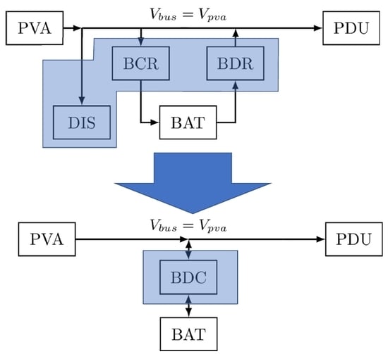
FRDET: In this implementation, the solar array is directly connected to the bus while the battery is interfaced with the bus using two different regulators, a charge regulator (BCR) and a discharge regulator (BDR). Since the bus is fully regulated, the operational point of the array is fixed, forcing the system to have a dissipation unit to consume excess energy production when the battery is fully charged. This system is complex, with a higher part count. This implementation is rarely used currently for lean satellites; this can be due to: (1) the complexity of the hardware, (2) the complexity of the control scheme; and (3) the lack of COTS solutions.

In order to reveal the current distribution of these implementations, a survey of the university-class satellite launches during 2016 is included in

Table 3. University-class satellite launches in 2016.

Name	Institution	Architecture	Size
HORYU-4	Kyushu Institute of Technology	BCPPT	10 kg
TOMSK-TPU120	Tomsk Polytechnic University	no data	3 U
AAUSAT4	Aalborg University	BCPPT	1 U
e-st@r-II	Polytechnic University of Turin	BCPPT	1 U
OUTFI-1	University of Liège	BCDET	1 U
SamSat-218/D	Samara State Aerospace University	BCPPT	3 U
BEESAT-4	Berlin Technical University	BCPPT	1 U
Sathyabamasat	Sathyabama University	BCPPT	2 U
Swayam	College of Engineering Pune	BCPPT	1 U
Aoxiang Zhixing	Northwestern Polytechnical University	BCPPT	12 U
3CAT-2	Universitat Politècnica de Catalunya	BCPPT	6 U
PISat	PES Institute of Technology	BCDET	5.3 kg
Pratham	Indian Institute of Technology Bombay	no data	10 kg
Opticube-4	California Polytechnic State University	dummy	2 U
RAVAN	Johns Hopkins Applied Physics Laboratory	BCPPT	3 U
Aoba-Velox-III	Kyushu Institute of Technology	BCPPT	2 U
EGG	University of Tokyo	no data	3 U
FREEDOM	Tohoku University	N/A 1	1 U
ITF-2	University of Tsukuba	BCDET	1 U
STARS-C	Shizuoka University	BCDET	1 U
Waseda-SAT 3	Waseda University	BCPPT	1 U
Totals2
	Architecture	BCDET	BCPPT
	Amount	4	12
	Percentage	25%	75%

¹ No solar panels, only battery. ² For projects that reported their architecture.

. The university-class was chosen because it is more likely to find detailed information about this type of project. In addition, the year 2016 was chosen considering that it takes some time for university teams to document their projects fully. In this case, the distribution was 25% BCDET and 75% BCPPT.

It is remarkable that not even one university project used the FRDET architecture in the chosen year, especially considering that this architecture is the standard in large spacecrafts, including most communication satellites and the International Space Station (ISS). This could be due to its complexity and lack of COTS solutions.

For this reason, the aims of this research are as follows: (1) to propose and develop an FRDET implementation that is better suited for lean satellites; and (2) to evaluate the performance of the proposed implementation by comparing it with the prevailing architecture implementations in the field of lean satellites.

In this work, a lean implementation of the FRDET architecture (Figure 2) is proposed as an alternative to the typical implementation. The system is based on a digitally-controlled bidirectional converter (BDC) that acts as a battery charger/discharger and bus voltage regulator. The BDC was realized by using two interleaved synchronous bi-directional buck converters (SBBC) working 180 degrees out of phase, as shown in Figure 3.

A simplified bidirectional transfer function of this converter is as follows:

$$V_{bat}\approx D·V_{bus},$$

(1)

where $V_{bat}$ is the voltage of the battery, $V_{bus}$ is the voltage of the bus, and D is the duty cycle of the pulse width modulated (PWM) signal that drives the BDC.

In the proposed implementation of the FRDET architecture, a reduction in part count was achieved by combining the BCR and BDR in a single bidirectional converter and by replacing the shunt regulator with a simple strategy to control excess energy. This would allow lean satellite developers to exploit the advantages of this architecture (see Table 2) without experiencing most of its disadvantages.

The results of this research showed that the proposed implementation of the FRDET architecture could harvest more solar power in a more efficient way in addition to being more reliable when compared to both the BCDET and the BCPPT architecture implementations.

2. Materials and Methods

In this work, an FRDET architecture based on a BDC is proposed as an alternative to the commonly used architectures, BCDET and BCPPT. Consequently, a direct comparison between these three architectures under the same conditions was done to evaluate the performance of the proposed solution. All the tests were designed to imitate a 1UCubeSat in an orbit equal to that of the ISS and tumbling in all axes at constant rates.

To ensure that the experiments were comparable, these three characteristics were set to be equal for all tests: (1) the photovoltaic array (PVA) illumination conditions, (2) the load power profile, and (3) the initial open circuit voltage (OCV) of the battery.

A solar array simulator (SAS) was used to simulate the PVA. An electronic load (ELO) was used to simulate the total consumption of all the loads. Both instruments were controlled with a period of one second using serial communication. The battery (BAT) consisted of two Li-ion cells in parallel. The rest of the test setup is detailed in Figure 4, where the dashed red and blue lines represent analog sensing data and the dashed green line is the PWM signal. Details of the materials and equipment are included in

Table 4. Materials and equipment details.

Block	Name	Model	Details
SAS	Solar array simulator	KEYSIGHT E4360A	Maximum: 600 W; 5 A; 130 V
ELO	Electronic load	KIKUSUI PLZ164WA	Maximum: 165 W; 33 A; 150 V
BAT	Battery	PANASONIC NCR18650B	Nominal: 3.6 V; 3200 mAh
VCS 1	Voltage and current sensors	Allegro ACS723LLCTR-05AB-T	$\pm 5$ A; 200 mV/V
DAQ	Data acquisition module	National Instruments USB-6211	16 AI, 2 AO, 4 DI, 4 DO
COU	Controller unit	Microchip PIC16F1786-ISP Texas Instruments TPS28225	8-bit Microcontroller Synchronous MOSFET Driver

¹ Voltage was measure with a simple voltage divider.

.

2.1. Prototype Board

For these experiments, a modular prototype board was fabricated as shown in Figure 5. It was comprised of: (1) a BDC realized with two interleaved SBBCs; (2) one controller unit (COU) consisting of a microcontroller and two MOSFET drivers for control of the BDC; (3) three voltage and current sensors (VCS); (4) a 5 V input to power the internal circuitry; (5) three pairs of banana plug connectors for SAS, ELO, and BAT connections; (6) a connector for sensor outputs to the data acquisition module (DAQ); and (7) a set of jumpers that allow the prototype to be configured according to each experiment.

2.2. SAS Setup and Control

The following assumptions were used for the simulation of the illumination conditions in orbit and the configuration of the SAS:

• The orbital parameters of the ISS were used (400 km of altitude, 51.6 deg of inclination).
• The date of the simulation was 23 September 2018, which corresponded to the autumn equinox.
• The rotation was considered constant in all axes with x = 0.2 deg/s, y = 0.1 deg/s and z = 0.2 deg/s.
• The configuration of the PVA was 2s5p, with 2 solar cells in series per each face in x, −x, y, −y, and z.
• The irradiance was assumed to be constant and equal to 1367 W/m².
• The chosen solar cell model was AZURSPACE 3G30A (see

  Table 5. AZURSPACE 3G30A datasheet data ¹.

  Configuration	1 Cell	2s3p (6 Cells)
  $V_{oc}$ (V)	2.69	5.38
  $I_{sc}$ (A)	0.52	1.56
  $V_{mp}$ (V)	2.41	4.82
  $I_{mp}$ (A)	0.50	1.51
  ${\eta }_{sc}$ (%)	29.3	29.3
  $A_{sc}$ (cm2)	30.18	181.08

  ¹ All electrical data at BOL and 1367 Wm⁻².

  ).
• The open circuit voltage ($V_{oc}$) and the maximum power voltage ($V_{mp}$) of the solar cell were assumed to be constant. Variations with solar incidence angle and temperature were ignored.
• The short circuit current ($I_{sc}$) and the maximum power current ($I_{mp}$) of the solar cell were assumed to be directly proportional to the cosine of the solar incidence angle.
• The base configuration of the SAS was 2s3p.

Although it is known that $V_{mp}$ is strongly affected by temperature, the variation was ignored because it would affect all three architectures in a similar way, and for that reason, it was not expected to affect the comparison, which was made with a dimensionless figure of merit introduced later in this section.

The chosen date provided the shortest possible sunlit time, which was the worst condition for the FRDET architecture because its efficiency was theoretically higher during the sunlit period of the orbit. This was done to ensure that any conclusions arising from the results of this paper could be generalized to any other date in the year.

The maximum available solar cell power at each instant is given by:

$$P_{sc}=\delta ·G_{SC}·A_{sc}·{\eta }_{sc}·\cos \left(\theta \right)$$

(2)

where $P_{sc}$ is the maximum available power of the solar cell, $\delta$ is the sunlight flag (sunlight = 1, eclipse = 0), $G_{SC}$ is the solar constant, $A_{sc}$ is the solar cell area, ${\eta }_{sc}$ is the efficiency of the solar cell, and $\theta$ is the solar incidence angle. This is only valid for angles from −90 deg to 90 deg.

Taking into consideration that a maximum of three faces can receive illumination at the same time, the available power of the PVA is:

$$P_{PVA}=\delta ·G_{SC}·A_{sc}·{\eta }_{sc}·\left[N_a·\cos \left({\theta }_a\right)+N_b·\cos \left({\theta }_b\right)+N_c·\cos \left({\theta }_c\right)\right],$$

(3)

where N is the number of solar cells per face and the subscripts a, b, and c identify the three illuminated faces at that instant.

In order to obtain a more useful expression, the available PVA power was normalized using, as the maximum value, the PVA power that would be obtained if three faces with two solar cells each were illuminated at maximum incidence ($\theta =0$), that is:

$$P_{6C}=6·G_{SC}·A_{sc}·{\eta }_{sc}.$$

(4)

This new normalized relation is given by:

$$pcos=\frac{P_{PVA}}{P_{6C}}=\delta ·\frac{N_a·\cos \left({\theta }_a\right)+N_b·\cos \left({\theta }_b\right)+N_c·\cos \left({\theta }_c\right)}{6},$$

(5)

where $pcos$ is called the pseudo-cosine and represents a normalized average of the contributions of all faces multiplied by the sunlight flag. Using this relation, Equation (3) is reduced to:

$$P_{PVA}=P_{6C}·pcos.$$

(6)

Having obtained this relation, an orbit simulation was run to obtain the pseudo-cosine every second for one orbital period using the previously mentioned assumptions, and the result is shown in Figure 6. Finally, the SAS was controlled by sending the following four parameters every second:

$$\begin{array}{cccc}\hfill V_{oc\left(SAS\right)}& =V_{oc\left(2s3p\right)};\hfill & \hfill I_{sc\left(SAS\right)}& =pcos·I_{sc\left(2s3p\right)};\hfill \\ \hfill V_{mp\left(SAS\right)}& =V_{mp\left(2s3p\right)};\hfill & \hfill I_{mp\left(SAS\right)}& =pcos·I_{mp\left(2s3p\right)}.\hfill \end{array}$$

(7)

The SAS received these parameters and used them to define its internal IV curve; its actual power output would depend on the impedance of the system at each instant. As an example, a set of curves for different $pcos$ values is shown in Figure 7; these curves were calculated using the same equations that the manufacturer used [4].

2.3. ELO Setup and Control

A distribution of the consumed power over an orbital period was generated in order to control the ELO. Five operation modes were defined as shown in

Table 6. Operation modes.

Mode	Power (W)	Dur.(s)	Rate 1
Stand-by (SB)	0.58	65	N/A
Beacon (BE)	0.78	30	28
Mission 1 (M1)	3.84	400	2
Mission 2 (M2)	1.35	200	3
Mission 3 (M3)	1.15	300	3

¹ Occurrences per orbital period.

. The distribution of those operation modes is shown in Figure 8.

During the experiments, the ELO was set in constant power (CP) mode and was controlled every second by sending the corresponding CP value according to Figure 8.

2.4. BDC Control

The BDC had a voltage control loop, which was implemented in the microcontroller of the COU using a digital PI controller. This control loop maintained a constant bus voltage ($V_{bus}$) of 4.8V for the BCPPT and FRDET configurations. The control period was 1ms.

2.5. BAT Preparation

Every set of experiments was done with the same initial OCV of the BAT. If the effects of aging, cycling, and temperature between each experiment were ignored, having the same OCV implied that the SOC was also the same. Each experiment was carried out at two different BAT OCVs; this was done because there were two important variables that were affected by this voltage:

• In the BCDET case, the harvested solar power was dependent on the voltage of the BAT; the higher the SOC, the higher the harvested solar power.
• In the BCPPT and FRDET case, the duty cycle of the converter was directly proportional to the voltage of the BAT.

To achieve this, the BAT was prepared before each experiment. A charger/discharger system developed by the authors [5] was used for this purpose.

2.6. Excess Energy Management Test

A final experiment was done to test the excess energy algorithm shown in Figure 9, where $V_{ref}$ is the bus voltage reference variable, $V_{set}$ is the normal bus voltage setpoint, $V_{bat}$ is the BAT voltage, $V_{fc}$ is the fully-charged BAT voltage setpoint, and $V_{sl}$ is the lower safe limit for the BAT voltage setpoint.

The battery was charged until it reached an OCV of 4.2V. The load profile was modified as shown in Figure 10 to have periods of high load power (Mission 1) followed by periods of low load power (stand-by and beacon) in order to see the reaction of the algorithm to these sudden changes when the battery was fully charged. For these tests: $V_{set}=4.8V$; $V_{fc}=4.15V$; and $V_{sl}=4V$. This algorithm was executed in a loop of 1ms, and the increments/decrements were 1mV.

2.7. Measurements and Calculations

2.7.1. Average System Efficiency

The efficiency was calculated every second using two different cases: if the cell was being charged, $P_{BAT}$ was positive, and the ratio was:

$$\eta =\frac{P_{out}}{P_{in}}=\frac{P_{ELO}+P_{BAT}}{P_{SAS}};$$

(8)

if the cell was being discharged, $P_{BAT}$ was negative, and the relation was:

$$\eta =\frac{P_{out}}{P_{in}}=\frac{P_{ELO}}{P_{SAS}-P_{BAT}}.$$

(9)

The average efficiency was calculated by adding up the instantaneous efficiency values over one orbital period as follows:

$$\overline{\eta }=\sum _{n=1}^{T_o}\frac{\eta }{T_o}.$$

(10)

where $T_o$ is the orbital period in seconds.

2.7.2. Average Relative Harvested Solar Power

The average harvested solar power was calculated by adding up the harvested solar power values over one orbital period as follows:

$$\overline{P_{SAS}}=\sum _{n=1}^{T_o}\frac{P_{SAS}}{T_o}.$$

(11)

The maximum solar power ($P_{MPP}$) is the power that could be harvested from the SAS at its maximum power point and can be calculated as follows:

$$P_{MPP}=pcos·I_{mp\left(2s3p\right)}·V_{mp\left(2s3p\right)}.$$

(12)

Its average over an orbital period is a constant and is given by:

$$\overline{P_{MPP}}=\sum _{n=1}^{T_o}\frac{P_{MPP}}{T_o}.$$

(13)

This maximum value was used to normalize the power input of the three architectures as follows:

$$\overline{RHSP}=\frac{\overline{P_{SAS}}}{\overline{P_{MPP}}}.$$

(14)

2.7.3. Weighted Efficiency

To compare the three different architectures under consideration in this work, a figure of merit was defined by combining the average system efficiency ($\overline{\eta }$) and the average relative harvested solar power ($\overline{RHSP}$) as follows:

$$w\eta =\overline{\eta }·\overline{RHSP},$$

(15)

where $w\eta$ is called the weighted efficiency.

2.8. Uncertainty

All the numerical results in this work originated either from a current or voltage measurement. The current sensor of VCS reported an uncertainty of ±2% [6]; the voltage signal originated from that sensor was then measured by the DAQ, which had an uncertainty of ±0.03% [7]. The VCS voltage signal was directly measured by the DAQ. The uncertainty propagation rules were then applied to the calculations to obtain the uncertainty of each numerical result as shown in

Table 7. Uncertainty of measurements and calculations.

Description	Symbol	Uncertainty
Voltage	V	$\pm 0.03\%$
Current	I	$\pm 2.03\%$
Power	P	$\pm 2.03\%$
Efficiency	$\eta$	$\pm 2.87\%$
Harvested solar power	$\overline{RHSP}$	$\pm 2.03\%$
Weighted efficiency	$W\eta$	$\pm 3.52\%$

.

2.9. Unmeasured Power Dissipation of the Controller Unit

The COU consisted of two devices: (1) a microcontroller; and (2) a synchronous MOSFET driver IC. These devices dissipated power during the operation of the BDC, but this power was not measured in the experiments because it was considered to be a small contribution to the stand-by consumption of the system and because it was provided by an external 5V line. An approximation of the COU consumption is included in

Table 8. COU power dissipation estimation.

Device	Description	Power (mW)
PIC16F1786	8 bit Microcontroller	12
TPS28225	MOSFET driver	100
COU	Total	112

.

3. Results

One aim of this research was to evaluate the electrical performance of the proposed FRDET architecture implementation for its use in lean satellite projects. This was done by comparing it with the common implementations of two widely used architectures in the field: BCDET and BCPPT.

The harvested SAS power for each experiment is shown in Figure 11, and the SAS voltage is shown in Figure 12. In the case of the BCPPT and FRDET architectures, the SAS voltage was regulated close to $V_{mp}$, and for that reason, the voltage profiles are overlapping in Figure 12. Because the SAS voltage was similar for BCPPT and FRDET, the harvested solar power was also similar and close to the maximum solar power ($P_{MPP}$); this can be seen in Figure 11 as both SAS power profiles are overlapping. For the previously stated reasons, in the BCPPT and the FRDET architectures, $\overline{RHSP}$ was similar to one, as seen in

Table 9. Summary of the results.

OCV	Arch.	$\overline{P_{ELO}}$ [W]	$\overline{\mathit{\eta }}$	$\overline{RHSP}$	$W\eta$
4.0 V	BCDET	1.31 ± 0.03	1.00 ± 0.03	0.86 ± 0.02	0.86 ± 0.03
	BCPPT	1.32 ± 0.03	0.90 ± 0.03	1.01 ± 0.02	0.92 ± 0.03
	FRDET	1.36 ± 0.03	0.93 ± 0.03	1.01 ± 0.02	0.94 ± 0.03
3.5 V	BCDET	1.30 ± 0.03	1.00 ± 0.03	0.76 ± 0.02	0.76 ± 0.03
	BCPPT	1.31 ± 0.03	0.90 ± 0.03	0.99 ± 0.02	0.90 ± 0.03
	FRDET	1.36 ± 0.03	0.95 ± 0.03	1.02 ± 0.03	0.96 ± 0.03

. In contrast, in the case of BCDET, the SAS was biased by the voltage of the BAT. The higher this voltage was, the higher the harvested power would be; this can be observed in Table 9. It is important to clarify that since the maximum voltage of the BAT (4.2 V) was below $V_{mp}$, it was not possible to harvest the maximum power of the SAS with the BCDET architecture.

The instantaneous power dissipated by the ELO over one orbital period is shown in Figure 13, and a summary of the load conditions is included in Table 9.

For each experiment, the setpoint value sent to the ELO every second was the same; however, the setup was different. This led to differences in the input noise and input impedance in the ELO, which could explain the small differences in the measured values. Let us consider the differences in the three configurations: (1) the BCDET case was the best case in terms of noise; the SAS output was well filtered, and the BAT was pure DC; (2) in the BCPPT case, the ELO was connected to the output of the BDC, which meant that it was affected by inductor current ripple noise; and (3) in the FRDET case, the ELO was connected to the input of the BDC, which meant that it was affected by the discontinuous nature of its input current, which also caused a ripple in the input of the ELO. Even with these differences, the ELO power profile was still similar for all the experiments, as can be observed in Figure 13.

The power balance of the BAT over one orbital period is shown in Figure 14. For the sake of clarity, an orange line that indicates zero watts is included in the BAT power balance plots. If the power value is above the orange line, the BAT is being charged; consequently, a power value below the orange line means that the BAT is being discharged.

4. Discussion

In the BCDET and BCPPT architectures, the BAT was simply clamped to the bus; in contrast, in the FRDET architecture, the BDC was located between the BAT and the bus; however, as can be seen in Figure 14, the transition between charge and discharge was seamless in all three architectures.

The effect of the lower power harvesting capabilities of the BCDET architecture can be observed in Figure 14. The amount of power that the BAT received during sunlit time was always lower than in the other two architectures, and the amount of power that it gave during that same period was higher. The lower the BAT voltage, the worse this effect would be, as can be seen in this same figure. It can be stated that, in the case of the BCDET architecture, as the BAT became more discharged, it became harder to recharge it.

For the BCPPT and the FRDET architectures, the power balance of the BAT was similar. Since the harvested solar energy was the maximum possible in both cases and the load profiles were equal in both cases, this behavior was expected. The differences arose in very specific operational conditions that will be analyzed later in terms of efficiency.

The instantaneous efficiency is shown in Figure 15. A summary of the results for each experiment is presented in Table 9.

The theoretical efficiency of the BCDET architecture was equal to one because there were only direct connections between the elements of the system (see Figure 1). As can be observed in Figure 15, it oscillated around that value, and finally, its average value was one, as shown in Table 9. It was observed that when the load power was higher (see Figure 13), the efficiency of the BCDET architecture went below one; this may indicate that there was a small power loss in the power traces of the fabricated prototype that became relevant as the power demand increased. This shall be reduced for future experiments by increasing the width of the power traces.

For the BCPPT architecture, the efficiency during an eclipse was expected to be close to one because during that period, the energy transfer between the BAT and the ELO was direct (see Figure 1; however, it was assumed that the internal consumption of the elements of the BDC in that condition was insignificant, and in the current setup, it could not be measured. As can be observed in Figure 15, that was not the case; instead, this internal consumption of the BDC was significant when compared with the stand-by and beacon operation modes of the ELO (see Figure 8), and that resulted in an efficiency of 80∼81% for the stand-by mode and 83∼85% for the beacon mode during eclipse. It was different when the ELO was in the Mission 1 operation mode; in that case, the efficiency was increased to 96∼97%. This meant that the internal consumption of the elements of the BDC became insignificant when compared to that operation mode. This effect could have been eliminated by using a diode in the output of the BDC in the BCPPT case, thus making the converter unidirectional; however, this would significantly affect the overall efficiency of the system during the sunlit period, and for that reason, it was discarded.

During the illuminated period, the FRDET architecture efficiency was expected to be higher than the BCPPT architecture efficiency because in that period, the FRDET architecture had direct energy transfer from the SAS to the ELO (see Figure 1). As expected, it was higher during the whole period. Nevertheless, it was still important to analyze the cases in which the BCPPT and FRDET architectures had similar efficiencies. That occurred when the BAT was supplying most of the power the ELO demanded because the SAS output power was low. Since the BCPPT architecture had direct energy transfer between the BAT and the ELO, that increased its efficiency in this condition, as shown in Figure 15 around Minute 10 and again around Minute 27.

During an eclipse, the FRDET architecture efficiency showed a different behavior for each OCV level. In the case of the 4.0V OCV, the efficiency during the stand-by (SB) and beacon (BE) modes oscillated around 85∼95%; in the 3.5 V case, it oscillated around 90∼95% for those same modes. This could be explained by considering that: (a) during an eclipse, the system efficiency was equal to that of the BDC; (b) the SB and BE modes were low power modes; (c) at light loads, the BDC converter entered into a condition called discontinuous conduction mode, which is known to reduce its efficiency [8].

The final experiment was designed to test the excess energy management algorithm. The load profile consisted of a repetition of a high-power period followed by a low-power period, as shown in Figure 16a. The voltage of the BAT started around 4.05V and decreased as it provided power to the load. After the ELO went to a low-power state, the BAT started charging, but when its voltage reached 4.15V, the algorithm started modifying the duty cycle to increase the SAS voltage setpoint, as can be seen in Figure 16c; this reduced the harvested power from the SAS, as can be seen in that same figure. The algorithm continued its control of the SAS voltage, reducing or increasing the setpoint to maintain the voltage of the BAT below 4.15V. This continued until the ELO entered a high-power mode again; in that moment, the BAT voltage was reduced, and the SAS voltage setpoint was constantly reduced until it reached the lower limit of 4.8V. This process was repeated until the eclipse period started. This experimental result confirmed the correct operation of the excess management algorithm.

5. Conclusions

At the beginning of this work, it was revealed that the traditional implementation of FRDET is rarely used currently for lean satellite designs. It was theorized that the reason for this was: (1) the complexity of the hardware; (2) the complexity of the control scheme; and (3) the lack of COTS solutions. Based on this, a new implementation of the FRDET architecture was proposed, prototyped, and evaluated. The proposed implementation was based on a digitally-controlled bidirectional converter (BDC) that acted as a battery charger/discharger and bus voltage regulator. Both the hardware and the control scheme had low complexity in the proposed solution.

The proposed FRDET implementation was evaluated in terms of its efficiency and harvested solar power by comparing it with the most common architectures in the field: BCDET and BCPPT. The BCDET architecture showed the highest average efficiency. BCDET was followed by FRDET and BCPPT, in that order. The FRDET and BCPPT architectures, however, could harvest the maximum amount of energy from the solar array, while the BCDET had a limited capability. In total, FRDET showed the highest weighted efficiency, which meant that this implementation was superior in electrical performance than both the BCPPT and the BCDET implementations. For a given load power requirement, the FRDET architecture could satisfy the requirements by the minimum number of solar cells.

In future research, a full characterization of the proposed FRDET implementation will be carried out over a wide range of operating conditions, this will include the effects of temperature and incident angle that were ignored in this work. Different implementations of the BDC are also considered for future work, including COTS solutions available on the market.